Rolling Bearing Fault Diagnosis Based on Nonlinear Underdetermined Blind Source Separation

Abstract

One challenge of bearing fault diagnosis is that the vibration signals are often a nonlinear mixture of unknown source signals. In addition, the practical installation position also limits the number of observed signals. Hence, bearing fault diagnosis is a nonlinear underdetermined blind source separation (UBSS) problem. In this paper, a novel nonlinear UBSS solution based on source number estimation and improved sparse component analysis (SCA) is proposed. Firstly, the ensemble empirical mode decomposition (EEMD), correlation coefficient (CC), and adaptive threshold singular value decomposition (ATSVD) joint approach is proposed to estimate the source number. Then, the observed signals are transformed into the time−frequency domain by short−time Fourier transform (STFT) to meet the sparsity requirement of SCA. The frequency energy is adopted to increase the accuracy of fuzzy C−means (FCM) clustering, so as to ensure the accuracy estimation of the mixing matrix. The L1−norm minimization is utilized to recover the source signals. Simulation results prove that the proposed UBSS solution can exactly estimate the source number and effectively separate the simulated signals in both linear and nonlinear mixed cases. Finally, bearing fault testbed experiments are conducted to verify the validity of the proposed approach in bearing fault diagnosis.

1. Introduction

Gearboxes have been widely used in many fields, such as aerospace, machine tool, automobiles, etc. As the core components of the gearboxes, gears and bearings are considered to be very prone to failure because of long−term operation under extreme conditions. A statistical report by Neale Consulting Engineers Ltd. showed that most gearbox failures (49%) are caused by the bearings, and the gears are considered as the second leading cause of failures (41%), followed by other components accounting for 10% of the failures [1]. The failure sequence frequently starts with a bearing, rather than a gear. The degradation and failure of bearings will cause a decline in performance and an increase in vibration, leading to overall damage to the rotating machinery system, economic losses, or even human casualties. Therefore, bearing fault diagnosis is of paramount importance to guarantee stable, reliable, safe operation of the machines and reduce avoidable economic losses. Bearing fault diagnosis techniques, including vibration signal analysis, acoustic analysis, and temperature monitoring, have been studied for many years [2]. Among these, vibration signal analysis has been widely developed because vibration signals contain abundant dynamic information about rotating machinery. Donelson and Dicus [3] adopted envelope analysis in the bearing fault diagnosis of freight cars. Pan and Tsao [4] utilized ensemble empirical mode decomposition (EEMD) and envelope analysis to detect the multiple faults of ball bearing. Cai [5] employed empirical mode decomposition (EMD) and high−order statistics to extract the fault features of rolling bearing in a Gaussian noisy environment. Wang et al. [6] proposed an improved EMD method, called EMD manifold, to enhance the fault detection of rotating machines. However, owing to the complexity of operating conditions, the traditional diagnostic techniques may not be able to make an accurate diagnosis, so more advanced diagnostic approaches should be developed.

As a research hotspot in signal processing over the past thirty years, blind source separation (BSS) has been widely used in many fields, including speech processing, vibration analysis, biomedical engineering, etc. [7]. It is an effective approach to obtain the source signal estimation from the observed signals (mixed signals) in the case where both the source signals and the mixing manner are unknown [8]. Since Gelle et al. [9] first introduced the BSS algorithm into rotating machinery fault diagnosis, more and more researchers have applied BSS theory to provide reliable fault diagnosis methods. Bouguerriou et al. [10] presented a BSS solution based on second order statistical properties and used it to detect the bearing faults. Li et al. [11] combined independent component analysis (ICA) with fuzzy k−nearest neighbor to diagnose the multi−faults of gears. Miao et al. [12] utilized median filter and the improved joint approximate diagonalization of eigenmatrices algorithm to identify the faults of rotating machinery. However, most studies mainly focus on the BSS problems in which the number of observed signals exceeds the number of source signals, namely the overdetermined BSS (OBSS) problem. In practice, the lack of prior knowledge about the sources makes it hard to pre−set the number of sensors that need to be installed. Meanwhile, objective factors such as the installation space of sensors will limit the collection of observed signals. Hence, the number of observed signals less than that of the source signals is in line with engineering practice, and it is imperative to seek the solution of underdetermined blind source separation (UBSS) for fault diagnosis in bearings.

Currently, some research work has been conducted to resolve the UBSS problem, which is mainly classified into two solutions [13]. The first one is to decompose the finite number of raw observed signals into multiple components through signal decomposition methods. Generally speaking, the number of multi−channel components is much larger than that of the source signals. Thus, the UBSS problem can be effectively converted into an overdetermined one, and then the ICA is employed to obtain the estimation of source signals. Another one takes advantage of the sparsity property of signals in the sparse domain, typically known as sparse component analysis (SCA), to resolve the UBSS in two stages: estimate the mixing matrix first and then recover the sources. In the first solution, the most commonly used decomposition methods are EMD, local mean decomposition (LMD), and variational mode decomposition (VMD), which have excellent performance when dealing with nonlinear signals [14]. The multi−channel components obtained by these decomposition methods are regarded as the virtual sensor outputs, hence the accuracy of the signal decomposition is crucial for source signal recovery. However, these decomposition methods still have some drawbacks. EMD suffers from mode mixing and end effect problems [15]. In the LMD algorithm, the calculation process of local mean function and local envelope function is accomplished based on the moving average method, which may lead to low decomposition efficiency and accuracy in processing non−stationary signals [16]. The performance of the VMD method relies largely on the appropriate choice of balance parameter and the number of decomposed modes [17]. These shortcomings may affect the accuracy of decomposition, resulting in inaccurate generation of virtual observed signals, and thus affect the recovery of source signals. In addition, although ICA is an operative method to solve the OBSS problem, it is necessary to strictly satisfy the assumption of the statistical independence of source signals. It is also assumed that the number of Gaussian components must be no more than one. Nevertheless, in engineering practice, the vibration signals do not always fulfill all assumptions, which limits the application scope of the ICA. Unlike ICA, SCA−based approaches do not require source independence or irrelevance, and sparsity of signals is the only requirement that needs to be met. Therefore, SCA is a more suitable method for dealing with the UBSS problem and can achieve better source separation performance, especially in rotating machinery fault diagnosis. Nevertheless, SCA−based approaches are difficult to implement with unknown source numbers. Furthermore, in the clustering stage, a large number of scatter points will increase the amount of computation and reduce the clustering accuracy, resulting in the failure to obtain accurate estimation of the mixing matrix.

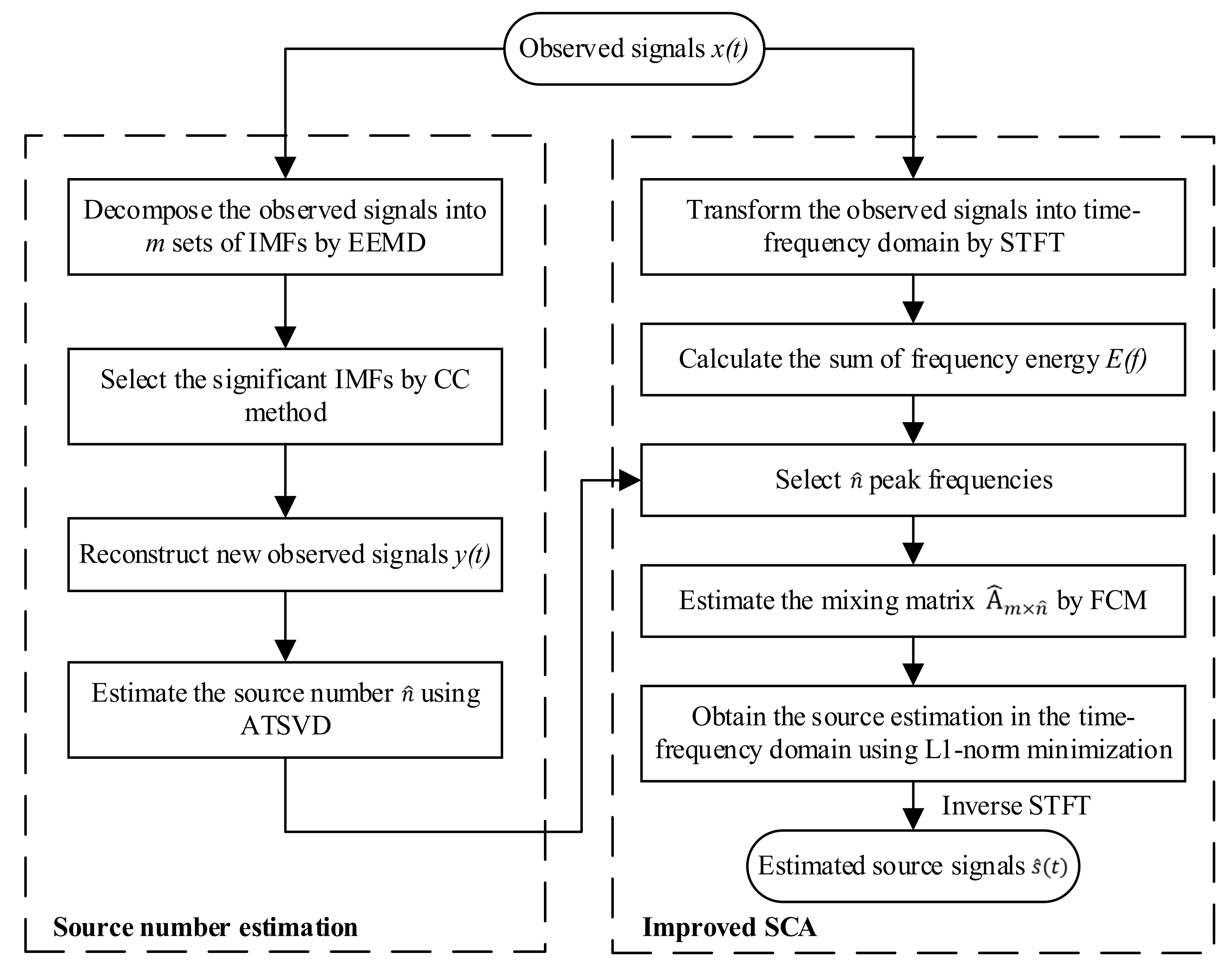
In terms of UBSS, it is urgent to solve the problem of determining how many source signals need to be recovered and how to accurately separate the observed signals. In this paper, a novel UBSS solution combining source number estimation and improved SCA is investigated for bearing fault diagnosis. Firstly, the EEMD and CC methods are adopted to obtain a group of significant IMFs. An eigenvalue method called adaptive threshold singular value decomposition (ATSVD) is adopted to obtain the number estimation of source signals. Secondly, short−time Fourier transform (STFT) is utilized to convert the observed signals into time−frequency domains. According to the obtained number estimation of source signals, the frequency energy is employed to reduce the amount of computation and improve the accuracy of fuzzy C−means (FCM) clustering, so as to ensure the accuracy estimation of the mixing matrix. Thirdly, the L1−norm minimization method is utilized to estimate the source signals. The numerical results demonstrate that the proposed method is able to effectively separate the simulated vibration signals, both in linear and nonlinear mixed cases, and can well identify the fault frequency in the inner race and outer race fault experiments.

The rest of this paper is organized as follows: Section 2 presents the source number estimation method based on the EEMD, CC, and ATSVD joint approach. Section 3 presents the mixing matrix estimation method based on the frequency energy and FCM clustering algorithm in detail and describes the source recovery by using L1−norm minimization. Section 4 evaluates the effectiveness and applicability of the proposed approach through simulation analysis. In Section 5, an inner race fault testbed experiment is conducted to validate the performance of the proposed approach in bearing fault diagnosis. Finally, the conclusions are drawn in Section 6.

2. Source Number Estimation Based on EEMD, CC, and ATSVD Joint Approach

Assuming that $x\left(t\right)=\left[x_1\left(t\right),x_2\left(t\right),\dots ,x_m\left(t\right)\right]$ are m−dimensional observed signals, which are generated by unknown source signals $s\left(t\right)=\left[s_1\left(t\right),s_2\left(t\right),\dots ,s_n\left(t\right)\right]$, the linear instantaneous mixed model of UBSS can be described as follows:

$$x\left(t\right)=\mathit{A}s\left(t\right)$$

(1)

where $\mathit{A}$ is an uncharted $m\times n$ linear mixing matrix, $m<n$, and $t$ represents the observation moment. The purpose of UBSS is to obtain the estimation of sources $\widehat{s}\left(t\right)={\left[\widehat{s_1}\left(t\right),\widehat{s_2}\left(t\right),\dots ,\widehat{s_n}\left(t\right)\right]}^T$ without any prior information of $\mathit{A}$ and $s\left(t\right)$. In general, the first step of SCA is to estimate the mixing matrix. If inaccurate mixing matrix estimation is generated, it will inevitably affect the separation result. Therefore, the mixing matrix estimation is the key to source signal recovery. 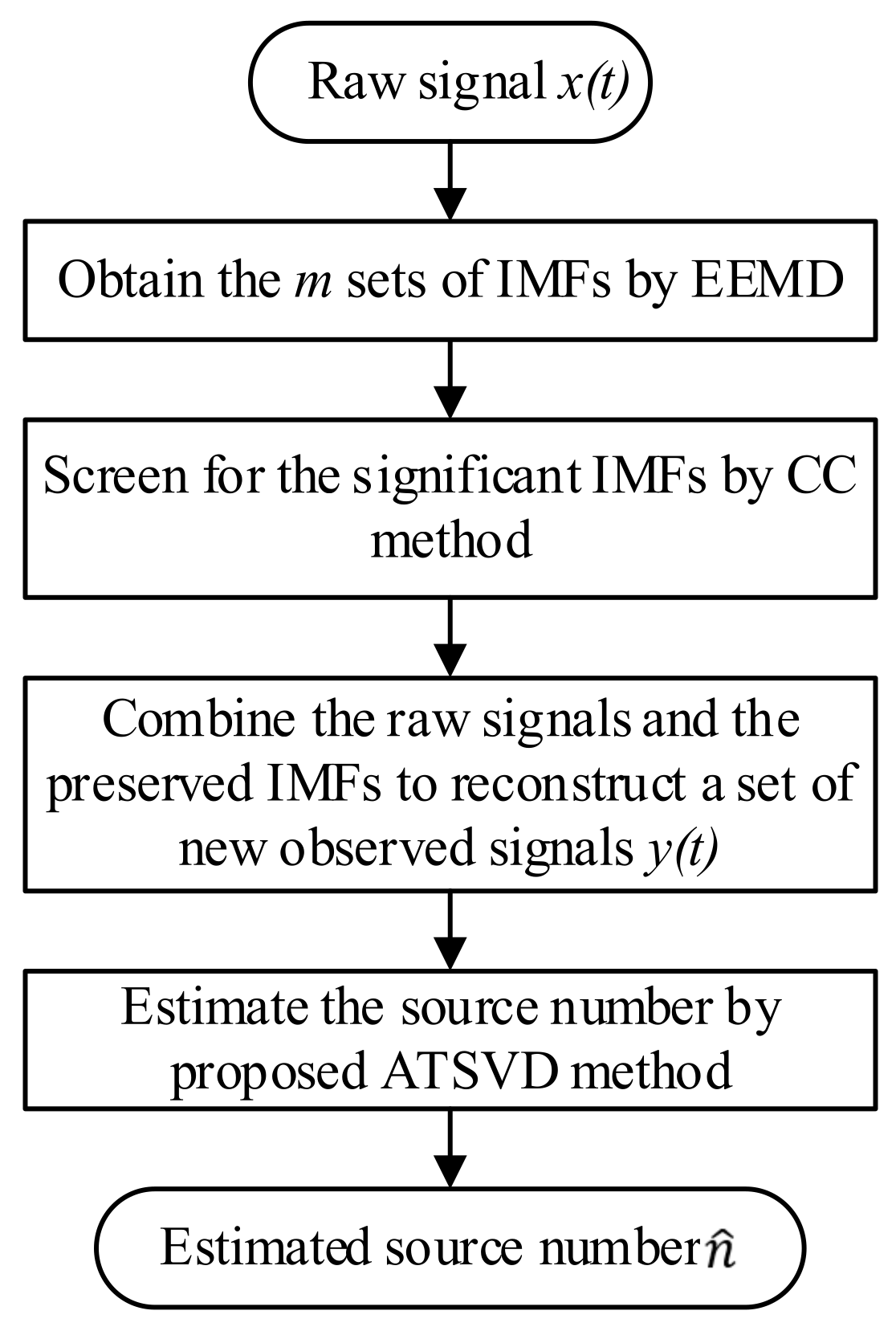The column number of $\mathit{A}$ represents the number of source signals, and hence the accuracy of source number estimation is crucial for mixing matrix estimation. In this section, a novel source number estimation approach based on EEMD, CC, and ATSVD is presented to convert the underdetermined source number estimation into an overdetermined one. Firstly, EEMD is utilized to decompose the original observed signals into $m$ sets of IMFs. Secondly, to remove the redundant IMFs and reduce the computational complexity, the CC method is utilized to screen for the significant components. Finally, an eigenvalue−based method named ATSVD is proposed to obtain the estimation of source number. The details are presented as follows.

2.1. Signal Decomposition Based on EEMD Algorithm

EMD is a powerful technique that can decompose a non−stationary and nonlinear signal into multiple IMFs. In general, each IMF is a mono−component function that satisfies the following conditions: (1) the number of extreme points (local minima and maxima) and that of zero crossing points must differ by one at most in the entire data set. (2) At any point, the mean of the upper and lower envelope must be zero [18]. Given one of the observed signals, $e\left(t\right)$, the EMD can decompose it as follows:

$$e\left(t\right)={\displaystyle \sum }_{j=1}^k{c}_j\left(t\right)+r\left(t\right)$$

(2)

where $c_j\left(t\right)$ is the obtained IMFs, $k$ denotes the number of IMFs, and $r\left(t\right)$ is the residue that denotes the central trend of $e\left(t\right)$.

Although traditional EMD is a powerful technique for processing non−stationary and nonlinear signals, it still has the mode mixing problem. To overcome the mode mixing issue, an improved EMD named EEMD was proposed by Wu and Huang [19]. The basic idea is to add several instances of white noise to the raw signal, so that the components of different scales can be automatically projected to the proper scale related to the white noise [14]. Given the observed signal, $e\left(t\right)$, the procedures of EEMD are listed as follows:

Step 1:

Add white noise, $n_1\left(t\right)$, to the observed signal, $e\left(t\right)$, and the mixed signal is:

$$e_1\left(t\right)=y\left(t\right)+n_1\left(t\right)$$

(3)

Step 2:

Use EMD to decompose the mixed signal, $e_1\left(t\right)$, into a group of IMFs as follows:

$$e_1\left(t\right)={\displaystyle \sum }_{j=1}^k{c}_{1j}\left(t\right)+r_1\left(t\right)$$

(4)

Step 3:

Add different white noise, $n_i\left(t\right)$ to $e\left(t\right)$, again and repeat Step 1 and Step 2 for $Ne$ times. Each time a new group of IMFs is acquired:

$$e_i\left(t\right)={\displaystyle \sum }_{j=1}^k{c}_{ij}\left(t\right)+r_i\left(t\right)$$

(5)

where $c_{ij}\left(t\right)$ is the jth IMF of the ith EMD trial.

Step 4:

Average the corresponding IMFs to eliminate the effect of the white noise, and the final result can be obtained:

$$e\left(t\right)={\displaystyle \sum }_{j=1}^k{c}_j\left(t\right)+r\left(t\right)$$

(6)

In this study, considering the computational cost and referring to parameter settings in some of the literature, the standard deviation of white noise is set as 0.2 times the raw signal, and the number of iterations, Ne, is set as 200 [20]. Thus, the raw signal can be effectively decomposed into a group of representative IMFs whose frequency bands are automatically arranged from high to low.

2.2. Significant Component Selection Based on the CC Method

The EEMD can effectively decompose a signal into a group of IMFs adaptively, with each IMF having the same length as the raw signal. However, the noise introduced during the decomposition process may cause the IMFs to contain redundant components [21]. To eliminate the influence of noise and reduce the subsequent computation, a simple selecting criterion called the correlation coefficient (CC) is employed to screen for the significant IMFs. The CC value can be calculated by the following formula:

$$Co{e}_{e\left(t\right),c_j\left(t\right)}=\frac{{{\displaystyle \sum }}_{i=1}^N\left(e\left(t\right)-\overline{e}\right)\left(c_j\left(t\right)-\overline{c_j}\right)}{\sqrt{{{\displaystyle \sum }}_{j=1}^N{\left(e\left(t\right)-\overline{e}\right)}^2}\sqrt{{{\displaystyle \sum }}_{j=1}^N{\left(c_j\left(t\right)-\overline{c_j}\right)}^2}}$$

(7)

where $e\left(t\right)$ is the raw signal and $\overline{e}$ denote the mean value of $e\left(t\right)$, $c_j\left(t\right)$ is the jth IMF and $\overline{c_j}$ denote the mean value of $c_j\left(t\right)$, and $N$ donates the number of the data points of $e\left(t\right)$. After calculation, the IMFs with significantly low CC values are screened out, and the preserved IMFs are the significant components that contain more defect information and the trend of the raw signal. Thus, each preserved IMF can be viewed as the output of a virtual sensor and treated as a new observed signal. Then, the preserved IMFs and the raw observed signals $x\left(t\right)$ are set as the new observed signals, which are rewritten as $y\left(t\right)={\left[y_1\left(t\right),y_2\left(t\right),\dots ,y_M\left(t\right)\right]}^T$, where $M$ is the sum of dimensions of the raw observed signals and the preserved IMFs. In this way, the UBSS problem can be effectively converted into an overdetermined one, and thus the source number estimation methods used in the overdetermined case can be applied.

2.3. Source Number Estimation Based on the ATSVD Method

In order to obtain accurate source recovery, the source number needs to be determined before the mixing matrix estimation. In previous research, some common information−based methods, such as Akaike information criterion and Bayesian information criterion, have been typically utilized to estimate the number of sources [14]. Nevertheless, these methods are only effective for estimating the source number in the white noise environment, but are invalid in the color noise environment. To ensure the accurate estimation of the mixing matrix, an eigenvalue method called ATSVD is proposed to estimate the number of source signals in this study. Firstly, the eigenvalues of the sample covariance matrix are obtained by singular value decomposition (SVD), then the source number is determined by the distribution of eigenvalues. In linear algebra, SVD is a commonly used matrix factorization technique that can decompose a matrix, $\mathit{X}\in R^{M\times M}$, into three matrices as follows:

$$\mathit{X}=\mathit{U}\mathit{S}{\mathit{V}}^T$$

(8)

where U and V represent $M\times M$ unitary matrices and S denotes an $M\times M$ diagonal matrix. The diagonal elements ${\lambda }_i$ of S are the eigenvalues of X and can be written in the descending order, e.g., ${\mathsf{\lambda }}_1\ge {\lambda }_2\ge \dots \ge {\lambda }_n\ge \dots \ge {\lambda }_M$. In general, the eigenvalues of source signal subspace ${\mathsf{\lambda }}_1~{\lambda }_n$ are much larger than the eigenvalues of noise subspace ${\mathsf{\lambda }}_{n+1}~{\lambda }_M$. At present, the two subspaces are usually distinguished by setting a threshold. However, the selection of threshold directly affects the accuracy of source number estimation. In this work, the estimation of source number is realized by calculating the contribution rate of eigenvalues. Given the new observed signals $y\left(t\right)={\left[y_1\left(t\right),y_2\left(t\right),\dots ,y_M\left(t\right)\right]}^T$, the key steps of the ATSVD algorithm can be summarized as follows:

Step 1:

Calculate the covariance matrix of $y\left(t\right)$ as follows:

$${\mathit{R}}_{yy}=E\left[y\left(t\right)y{\left(t\right)}^H \right]$$

(9)

where ${ }^H$ represents the complex conjugate transpose.

Step 2:

Decompose the covariance matrix, ${\mathit{R}}_{yy}$, by SVD to obtain the eigenvalues ${\mathsf{\lambda }}_1~{\lambda }_M$, then remove eigenvalues less than 0.001, and the retained eigenvalues are used to constitute a new eigenvector of length $l$.

Step 3:

Sum all the eigenvalues and then calculate the ratio of each eigenvalue, i.e., contribution rate:

$$d_i=\frac{{\lambda }_i}{{{\displaystyle \sum }}_{i=1}^l{\lambda }_i},i=1,2,\dots ,l$$

(10)

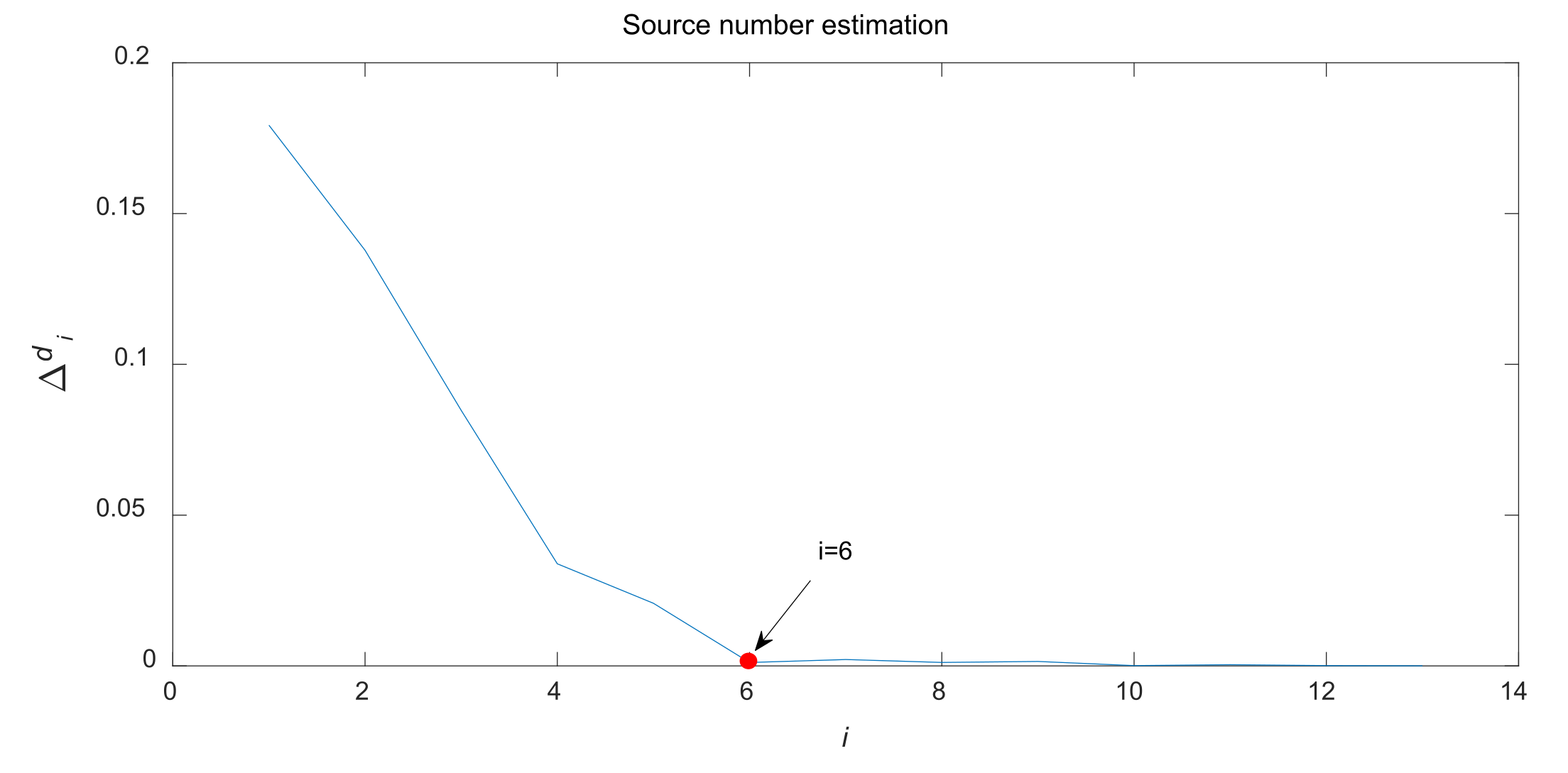
Step 4:

Calculate the difference between the two adjacent contribution rates:

$$\mathrm{\Delta }{d}_i=d_i-d_{i+1},i=1,2,\dots ,l-1$$

(11)

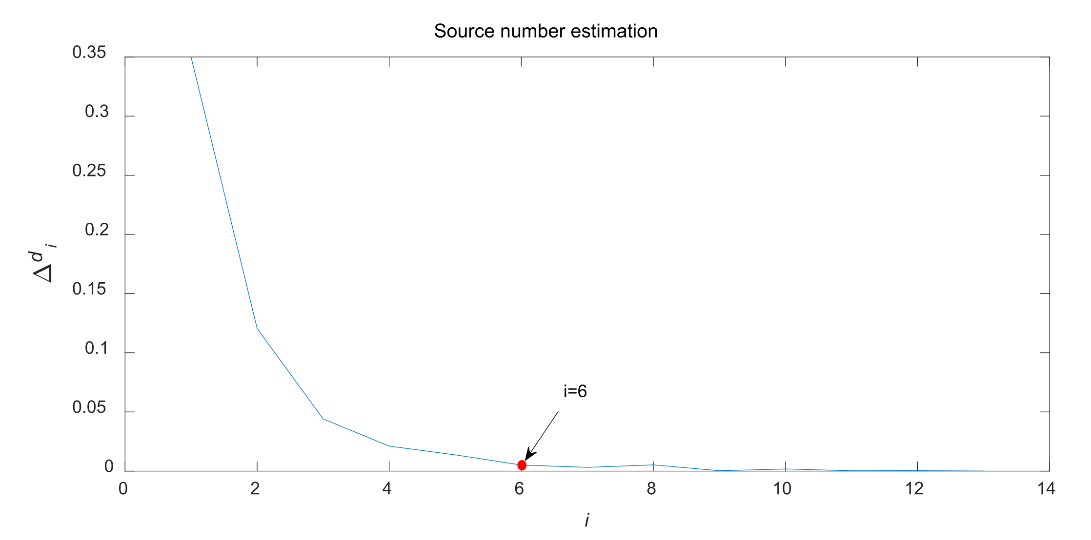
Herein, the maximum value ($\mathrm{\Delta }{d}_i)$ is set as the threshold to distinguish the source signal subspace and noise subspace, and $i$ is the estimated number of sources. In summary, the procedure of source number estimation is described as Figure 1. Based on the estimated number, $\widehat{n}$, the number of clustering centers can be determined in advance.

3. Source Signal Recovery Based on Improved SCA

SCA is an effective approach to resolving the UBSS problem and has been widely applied in vibration analysis, image processing, modal identification, etc. Signal sparsity refers to the fact that most points in the signal are zero or near zero, but a few points are obviously greater than zero. However, most vibration signals cannot meet the sparse requirement in the time domain. In order to improve the sparsity of the observed signals, STFT is first carried out to convert the signals from the time domain to the time−frequency domain. In engineering, the frequency of each source signal is usually different to avoid resonance. Therefore, there is generally only one source at a specific time−frequency point. It must be emphasized that although the gearbox is a nonlinear system, such nonlinearity will not affect the defect frequency, hence SCA is able to reserve the fault information in the time−frequency domain. In this section, an improved SCA is employed to separate the mixed signals. Firstly, FCM clustering is adopted to estimate the mixing matrix, and frequency energy is employed to improve the clustering accuracy. Secondly, the L1−norm minimization method is utilized to estimate the source signals. The details are presented as follows.

3.1. Mixing Matrix Estimation Based on FCM and Frequency Energy

Mixing matrix estimation is the most critical part of the SCA because the estimated mixing matrix determines the accuracy of signal separation. In the literature, the main methods of mixing matrix estimation are the potential function method and the clustering method. The potential function method expands the angle of the clustering line to the polar coordinate axis and determines the angle between the clustering line and the coordinate axis by calculating the peak value points, so as to obtain the column vectors of the mixing matrix. However, it can only be used for two−channel mixed signals, which has certain limitations. In contrast, the clustering method determines the mixing matrix by estimating the center of the clustering line, which is not limited by the number of channels. Currently, the most−used clustering algorithms are K−means and FCM. The former is a hard partition−based clustering method, while the latter is a soft partition derived from the fuzzy set theory [22]. In this work, FCM clustering is selected to realize the mixing matrix estimation because the strict attributes are usually not available for vibration signals.

Denote $X=\left\{x_1,x_2,\cdots , x_n\right\}$ as a set of limited observation sample. The FCM is a clustering algorithm that can produce membership degree $u_{ij}=u_i\left(x_j\right)\in \left[0, 1\right]$ for each data point. The objective function of FCM is given as follows:

$$J={\displaystyle \sum }_{i=1}^c{\displaystyle \sum }_{j=1}^n{u}_{ij}^a\Vert x_j-v_i\Vert {}^2$$

(12)

where $c$ is the cluster number, $n$ is the number of data points in $X$, and $a$ denotes a fuzzy partition matrix exponent for controlling the degree of fuzzy overlap, with $a>1$. Fuzzy overlap refers to how fuzzy the boundaries between clusters are, that is the number of data points that have significant membership in more than one cluster; $x_j$ is the jth data point, $v_i$ is the center of the ith cluster, and $u_{ij}$ is the membership degree of $x_j$ in the ith cluster, which satisfies ${{\displaystyle \sum }}_{i=1}^n{u}_{ij}=1, j=1, 2, \dots , n$.

Then, the Lagrange multiplier method is adopted to minimize the objective function. The degree of membership and the centers of clusters can be updated by the following formulas:

$$u_{ij}=\frac{1}{{{\displaystyle \sum }}_{k=1}^c{\left(\frac{\Vert x_j-v_i\Vert }{\Vert x_j-v_k\Vert }\right)}^{\left(\frac{2}{a-1}\right)}}$$

(13)

and

$$v_i=\frac{{{\displaystyle \sum }}_{j=1}^n{u}_{ij}^a{x}_j}{{{\displaystyle \sum }}_j^n{u}_{ij}^a}$$

(14)

The procedures of FCM clustering can be listed as follows:

Step 1:

Fix the number of clusters, $c$, the value of the fuzzy partition matrix exponent, $a$, and the iteration deadline error, $\epsilon$;

Step 2:

Initialize the degree of membership matrix, $\mathit{U}=\left[u_{ij}\right]$;

Step 3:

Calculate the clustering center matrix, $\mathit{V}=\left[v_i\right]$, based on Equation (14);

Step 4:

Update the degree of membership matrix, ${\mathit{U}}^{\prime }$, based on Equation (13);

Step 5:

Compare $\mathit{U}$ and ${\mathit{U}}^{\prime }$; if $\Vert \mathit{U}-{\mathit{U}}^{\prime }\Vert <\epsilon$, terminate the iteration; otherwise update $\mathit{U}={\mathit{U}}^{\prime }$ and return to Step 3.

FCM is an excellent clustering algorithm with a mature theory and wide applications. Nevertheless, the actual collected signals are mixed by multiple source signals, resulting in more clustering directions in the scatter graph. When the number of data points is too large in the process of clustering, it will not only increase the computational burden but also affect the clustering accuracy, resulting in the inability to obtain an accurate mixing matrix. To address this issue, a simple method, namely frequency energy, is adopted to improve the accuracy of mixing matrix estimation [23,24]. In engineering practice, the energy of vibration signals is generally concentrated at some frequency points, and the clustering direction at the local maximum frequency points can be used as the clustering direction of the source signals. Thus, the estimated mixing matrix can be obtained only by finding the clustering direction at these peak frequency points, which can significantly reduce the amount of computation and increase the accuracy of clustering. In this work, the energy distribution of each observed signal is first calculated, and then the energy distribution of all the observed signals is added at the same frequency point; that is:

$$E\left(f\right)={\displaystyle \sum }_{i=1}^m{{\displaystyle \int }}_{-\infty }^{\infty }\left\{R{\left[x_i\left(t,f\right)\right]}^2+I{\left[x_i\left(t,f\right)\right]}^2\right\}dt$$

(15)

where $E\left(f\right)$ denotes the energy sum of all the observed signals at each frequency point and $m$ is the number of observed signals; $R\left[x_i\left(t,f\right)\right]$ and $I\left[x_i\left(t,f\right)\right]$ represent the real and imaginary parts of the ith sensor signal after STFT, respectively.

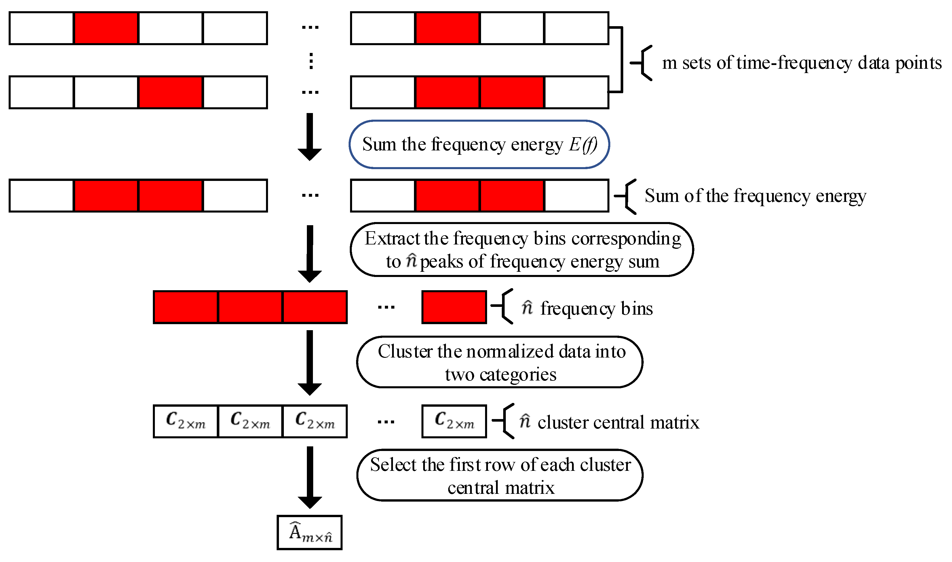
In summary, the schematic diagram of the mixing matrix estimation is presented in Figure 2 and the steps can be listed as follows:

Step 1:

Adopt STFT to transform the observed signals into the time−frequency domain, and the matrix expression can be denoted as $x_i\left(t, f\right)$, where $i=1, 2, \dots , m$, and $m$ is the number of observed signals;

Step 2:

Calculate the sum of the energy, $E\left(f\right)$, and then utilize the peak detection method to select $\widehat{n}$ peaks of frequency energy sum ($f_1, f_2, \dots , f_{\widehat{n}}$), where $\widehat{n}$ is the estimated source number;

Step 3:

Select the data points of a certain frequency (e.g., from $f_1$ to $f_{\widehat{n}}$) to form a new matrix, $\mathit{V}$;

Step 4:

Normalize $\mathit{V}$, then utilize FCM to divide it into two categories, and the cluster central matrix can be represented as ${\mathit{C}}_{2\times m}$. The first row of ${\mathit{C}}_{2\times m}$ is selected as a column vector of the estimated mixing matrix;

Step 5:

Alter the frequency and repeat Step 3 and Step 4 $\widehat{n}$ times; the estimated mixing matrix $\hat{\mathit{A}}$ of $m\times \widehat{n}$ can be obtained.

3.2. Source Signal Recovery Based on L1−Norm Minimization

According to the estimated mixing matrix, $\hat{\mathit{A}}$, the estimated source signals can be obtained by $\widehat{s}\left(t\right)={\hat{\mathit{A}}}^{-1}x\left(t\right)$ in the overdetermined or determined case. However, in the underdetermined case, there are still multiple valid solutions despite the determination of the mixing matrix. Previous studies have confirmed that the solution derived from the minimum of L1−norm is the optimal solution of the underdetermined system of equations [25]. Thus, the source recovery problem can be converted into an optimization problem. The estimated mixing matrix, $\hat{\mathit{A}}$, can be generated into $C_{\widehat{n}}^m$ $m\times m$ submatrices by reducing dimensions, and these submatrices correspond to $C_{\widehat{n}}^m$ sets of valid solutions. The optimal solution fulfilling the following equation can be obtained among all valid solutions:

$$\left\{\begin{array}{c}\widehat{s}\left(t, f\right)=min{\displaystyle {\displaystyle \sum }_{i=1}^{\widehat{n}}}\left|s_i\left(t,f\right)\right|\\ s.t. \hat{\mathit{A}}s\left(t,f\right)=x\left(t,f\right)\end{array}\right.$$

(16)

where $\hat{s}\left(t,f\right)$ is the optimal source estimation in the time−frequency domain. The main steps of the L1−norm minimization method can be summarized as follows:

Step 1:

Generate $C_{\widehat{n}}^m m\times m$ submatrices from the estimated mixing matrix $\hat{\mathit{A}}$ and set as ${\mathit{B}}_k, k=1,2,\dots , C_{\widehat{n}}^m$;

Step 2:

Denote $\mathit{X}$ as a point in the time−frequency domain, calculate all possible solutions ${\widehat{\mathit{S}}}_k={\mathit{B}}_k^{-1}\mathit{X}, k=1,2,\dots , C_{\widehat{n}}^m$;

Step 3:

Calculate the L1−norm of each solution, and the minimum L1−norm is taken as the optimal estimation of the source signal, which is given by $\widehat{\mathit{S}}=\min {\displaystyle \sum }_{i=1}^{C_{\widehat{n}}^m}\left|{\left({\widehat{\mathit{S}}}_k\right)}_i\right|$;

Step 4:

Repeat Step 2 and Step 3 and the optimal source estimation in the time−frequency domain can be obtained;

Step 5:

Perform inverse STFT to obtain the estimated source signals in the time domain.

In summary, the flowchart of the proposed UBSS solution is illustrated in Figure 3.

4. Simulation and Results

This section presents the simulation to verify the separation performance of the proposed UBSS approach, in both linear and nonlinear cases.

4.1. Simulation Settings

In simulations, according to the vibration analysis in [26], the vibration signals generated by the faulty bearing can be expressed as follows:

$$s_{bearing}\left(t\right)=\mathit{sin}\left(2\pi f_{bearing}t\right)\times \left(1+\alpha \times \mathit{sin}\left(2\pi f_{r}t\right)\right)$$

(17)

where $f_{bearing}$ is the fault frequency of the bearings. The vibration signals caused by gear meshing can be generated by the following model:

$$s_{gear}\left(t\right)={\displaystyle \sum }_{k=1}^K{A}_k\left(t\right)\mathit{cos}\left(2\pi k{f}_{mesh}t+{\varphi }_k\left(t\right)\right)$$

(18)

where $A_k\left(t\right)$ denotes the instantaneous amplitude modulation, $f_{mesh}$ is the meshing frequency, and ${\varphi }_k\left(t\right)$ represents the instantaneous phase modulation. The pulse signals produced by the mechanical vibration shock can be modelled as:

$$I\left(t\right)=e^{-\lambda t}s\left(t\right)$$

(19)

where $\lambda$ is a constant.

In this study, five raw source signals that can well represent the vibration of the gearbox under the actual working conditions are generated, respectively: $s_1\left(t\right)$ and $s_2\left(t\right)$ are modulated signals generated based on Equation (17), $s_3\left(t\right)$ and $s_4\left(t\right)$ are periodic signals generated based on Equation (18), and $s_5\left(t\right)$ is an impulse signal generated based on Equation (19). The generated signals are given as follows:

$$\begin{gathered} s_1\left(t\right)=\left(\mathit{cos}\left(2\pi f_{0}t\right)+1\right)\times \mathit{sin}\left(2\pi f_{1}t\right) \\ {s}_2\left(t\right)=\left(\mathit{cos}\left(2\pi f_{0}t\right)+1\right)\times \mathit{sin}\left(2\pi f_{2}t\right) \\ {s}_3\left(t\right)=sin\left(2\pi f_{3}t\right) \\ {s}_4\left(t\right)=sin\left(2\pi f_{4}t\right) \\ {s}_5\left(t\right)=\mathit{sin}\left(2\pi f_{5}t\right)\times e^{-\lambda t_1}, t_1=mod\left(t,0.25\right) \end{gathered}$$

(20)

where $f_0=10 \mathrm{Hz}$, $f_1=50 \mathrm{Hz}$, $f_2=150 \mathrm{Hz}$, $f_3=100 \mathrm{Hz}$, $f_4=200 \mathrm{Hz}$, $f_5=400 \mathrm{Hz}$, and $\lambda =50$. The sampling time and frequency are set as 1 s and 1024 Hz, respectively. The waveform of the simulated signals in the time and frequency domains is presented in Figure 4.

4.2. UBSS for Linear Mixed Signals

In this section, to validate the effectiveness of the proposed approach in the linear mixed case, the simulated signals are mixed by a random matrix, ${\mathit{A}}_{3\times 5}$, and the waveform of the mixed signals in the time domain is shown in Figure 5. In the source number estimation procedure, EEMD, CC, and ATSVD are used for processing the simulated signals. Based on the EEMD, each mixed signal can be decomposed into a group of representative IMFs. The CC values between the IMFs and the original signal, $x\left(t\right)$, are calculated, and the result is shown in

Table 1. CC values between each IMF and the raw signals.

IMF	C1	C2	C3	C4	C5	C6	C7	C8	C9
$x_1\left(t\right)$	0.8153	0.4263	0.3541	0.1161	0.0131	0.0071	0.0056	0.0030	0.0000
$x_2\left(t\right)$	0.8820	0.4549	0.1878	0.0349	0.0233	0.0167	0.0147	0.0070	0.0005
$x_3\left(t\right)$	0.8395	0.4485	0.3751	0.1383	0.0130	0.0074	0.0090	0.0039	0.0004

. Taking the signal $x_2\left(t\right)$ as an example, the EEMD decomposes it into nine IMFs, C₁–C₉, and one residue. It can be seen that the CC values of C₁–C₃ are much higher than those of C₄–C₉. Theoretically, a higher CC value means that the IMF contains more information about the raw signal. Hence, C₁–C₃ are selected to represent the raw signal features, and the rest of the IMFs are treated as noises and screened out. After calculating all CC values, it is observed that for $x_1\left(t\right)$ and $x_3\left(t\right)$, the original signals are also closely related to only the first four IMFs. Therefore, these eleven IMFs are chosen to reconstruct the new observed signals combined with the original signals.

After obtaining the newly observed signals, the UBSS problem can be effectively transformed into an overdetermined one. Then, the ATSVD method is utilized to estimate the source number, and the result is shown in Figure 6. It can be seen that the eigenvalue becomes relatively close to zero after $i=6$. Therefore, the estimated source number is five.

Based on the obtained source number, the improved SCA method is utilized to recover the source signals. Figure 7 shows the waveform of the five recovered signals in the time and frequency domain. It is obviously that the waveform and the main characteristic frequency of each recovered signal are consistent with those of the corresponding source signal, indicating that the proposed approach performs well in recovering the source signals. Furthermore, the CC method is employed to evaluate the separation performance. The CC values between the recovered signals and the corresponding source signals are presented in

Table 2. CC values between the recovered signals and the corresponding source signals.

Index	CC Values
1	0.9902
2	0.9956
3	0.9947
4	0.9958
5	0.9995

. It can be seen that each CC value is close to 1, which confirms the effectiveness of the proposed approach in separating the linear mixed signals.

4.3. UBSS for Nonlinear Mixed Signals

In this section, the separation performance of the proposed approach in the nonlinear mixed case is validated. In practice, the vibration signals in the gearbox are often mixed in a nonlinear manner. Nevertheless, such nonlinearity will not affect the fault characteristic frequencies, and hence the proposed method can be adopted in the nonlinear mixed case directly. In simulation, the post−nonlinear mixed model is adopted as follows:

$$x\left(t\right)=f\left(\mathit{A}s\left(t\right)\right)$$

(21)

where $f$ represents a nonlinear function and $\mathit{A}$ denotes a random matrix of $3\times 5$. In this work, the hyperbolic tangent function is employed to distort the mixed signals, which is given as follows:

$$f=\tanh ()$$

(22)

Three mixed signals, $x_1-x_3$, are shown in Figure 8. After calculating the CC values between the IMFs and the original signal, $x\left(t\right)$, the first three IMFs, C₁–C₃, of $x_1$ and the first four IMFs, C₁–C₄, of $x_2\left(t\right)$ and $x_3\left(t\right)$ are preserved to construct the new observed signals combined with the original signals. Figure 9 gives the result of source number estimation. It can be observed that the eigenvalue becomes relatively close to zero after $i=6$, and hence the estimated source number is five. The simulation results prove that the proposed source number estimation approach can perform fairly well, in both linear and nonlinear cases.

Based on the estimated source number, five estimated source signals are obtained, and the time−domain waveforms and frequency spectra are presented in Figure 10. It can be seen that the waveform of each recovered signal is basically the same as the corresponding source signal, except for the amplitude change. Moreover, the feature frequency of each recovered signal is consistent with that of the corresponding source signal. The results prove that the proposed approach is able to well separate the nonlinear mixed signals. Furthermore,

Table 3. CC values between the recovered signals and the corresponding source signals obtained by different methods.

Index	Proposed Solution	Solution in [27]
1	0.9264	0.8137
2	0.9521	0.5388
3	0.9699	0.9329
4	0.9958	0.7813
5	0.8934	0.7236
Average	0.9475	0.7581

presents the CC values between the recovered signals and the corresponding source signals for the proposed approach by using the existing nonlinear UBSS solution in [27] as the comparison benchmark. It can be seen that although the CC values have a certain decrease compared with the linear mixing case, the average CC value of the proposed solution is much higher than that of the benchmark solution, which demonstrates that the proposed approach performs much better than the existing UBSS solution in tackling nonlinear mixed signals.

5. Experiment and Results

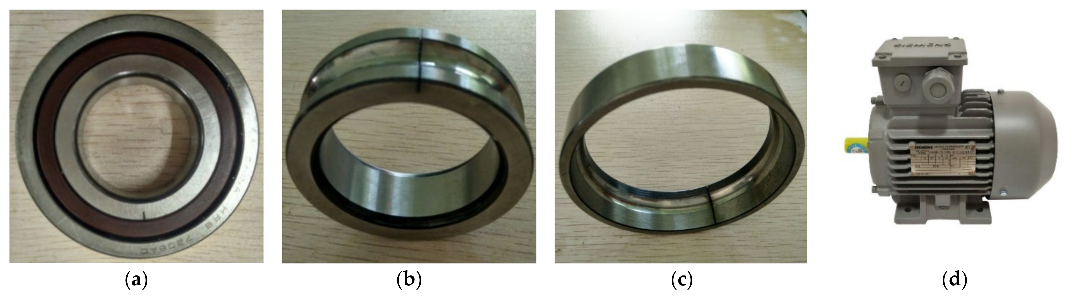
This section carries out the bearing fault testbed experiments to verify the separation performance of the proposed approach for actual measured signals. The rolling bearing fault testbed consists of a rolling bearing, two acceleration sensors, and an alternating current (AC) variable frequency motor. Figure 11a shows the tested rolling bearing; the type is HRB 7208AC. In order to simulate the bearing fault in actual working conditions, two types of single point fault, which are inner race fault and outer race fault, are artificially introduced to the tested bearing by means of electrical discharge machining. Figure 11b,c present the faulty inner ring and outer ring, respectively. It can be seen that there is an artificial gap of 2 mm in both the inner and outer rings. The bearing is preloaded axially. The sensors are installed on the bearing housing; the type is CA–YD–182. The motion in the test is generated by an AC variable frequency motor, which is shown in Figure 11d; the type is SIEMENS 1LE0001–0DB32. The rotating speed is set to 4000 rpm and the vibration signals are acquired by the dynamic signal analyzer. The sampling frequency is 4000 Hz, and 1 s is intercepted as a time fragment.

Table 4. Parameters of the gearbox.

Parameters	Value
Bearing specs	$\mathrm{HRB} 7208\mathrm{AC}$
$\mathrm{Ball} \mathrm{diameter} D_b$	11.1 mm
$\mathrm{Pitch} \mathrm{circle} \mathrm{diameter} D_p$	$61.4$ mm
Roller number N	$13$
Contact angle ϕ	${25}^{°}$
$\mathrm{Shaft} \mathrm{rotation} \mathrm{frequency} f_r$	40 Hz

presents the specifications and parameters of the tested bearing. When the bearing is running, the fault feature frequency of the rolling bearing is the recurrence frequency of the vibration pulse generated via the contact between the defect and the raceways or rollers. The fault characteristic frequencies of a rolling bearing can be obtained by the following theoretical formula:

$$f_{bpfi}=\frac{N}{2}\left(1+\frac{D_{b}cos\varphi }{D_p}\right)f_r$$

(23)

$$f_{bpfo}=\frac{N}{2}\left(1-\frac{D_{b}cos\varphi }{D_p}\right)f_r$$

(24)

where $f_{bpfi}$ represents the frequency of the inner race fault point passing each rolling element and $f_{bpfo}$ represents the frequency of the outer race fault point passing each rolling element. The calculation results are 302.6 Hz and 217.4 Hz, respectively.

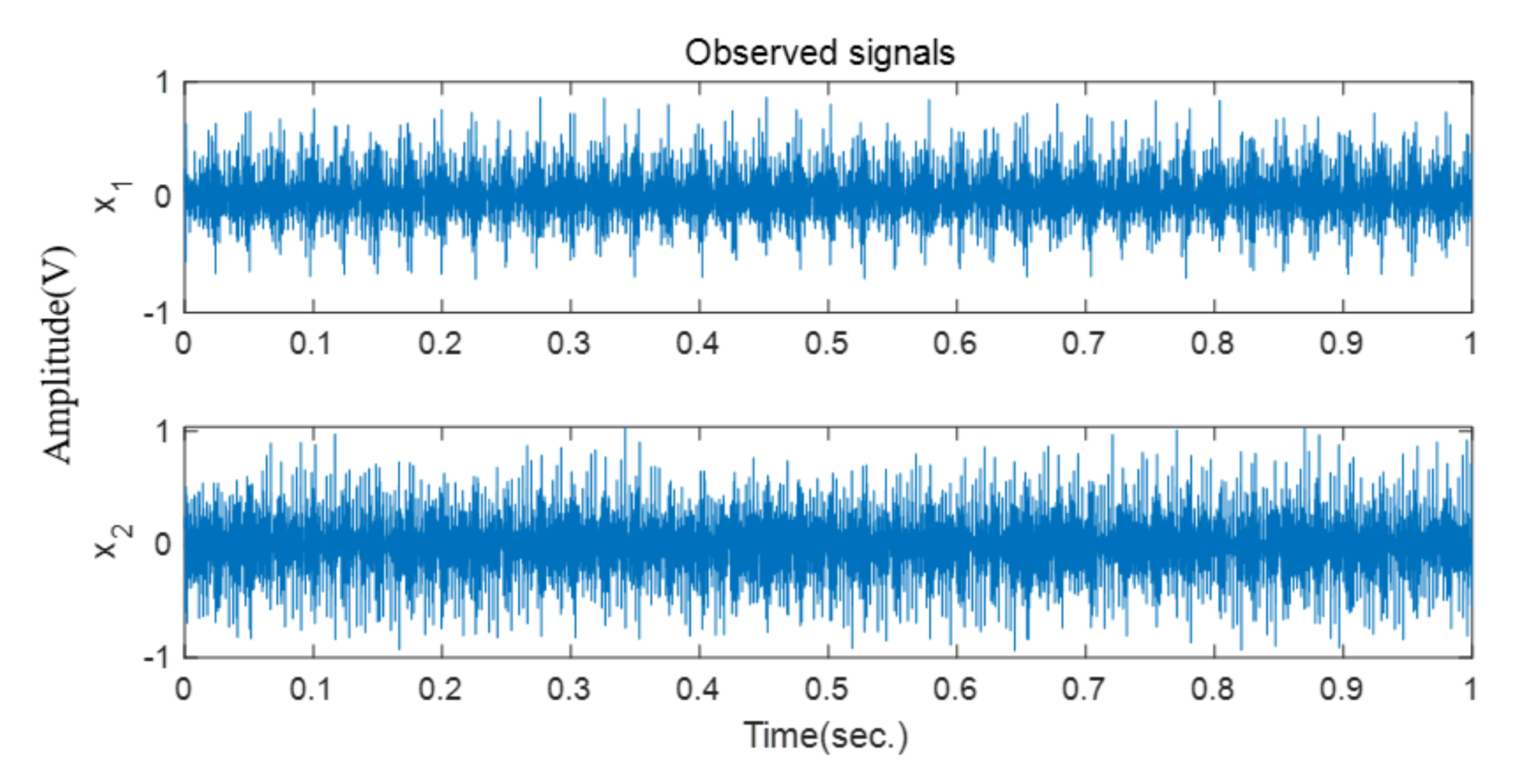
5.1. Inner Race Fault

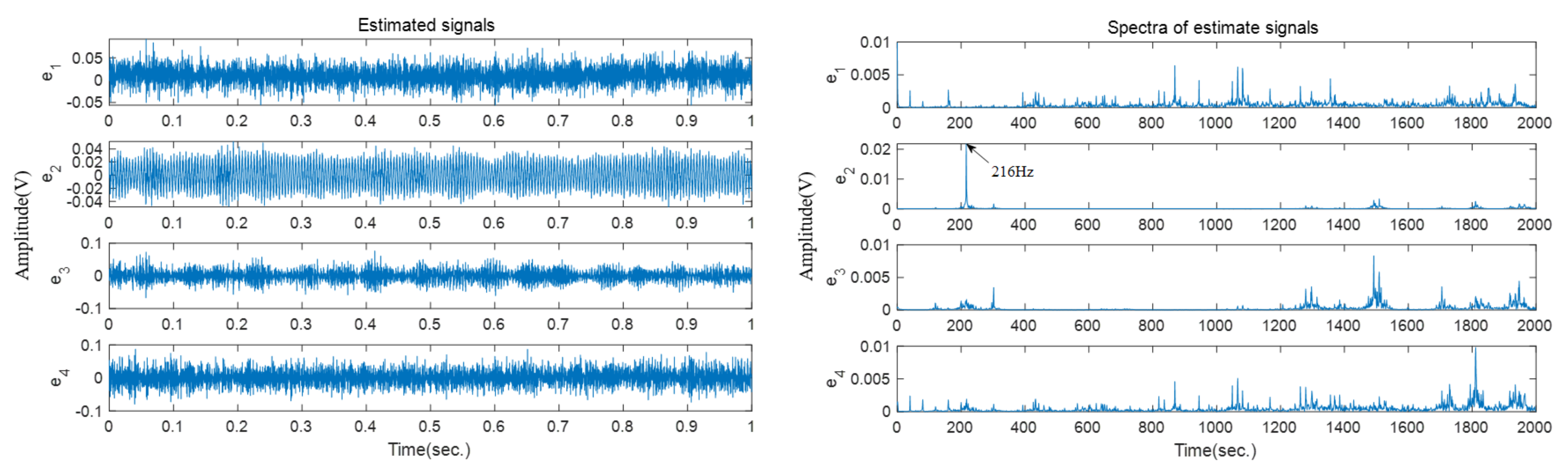
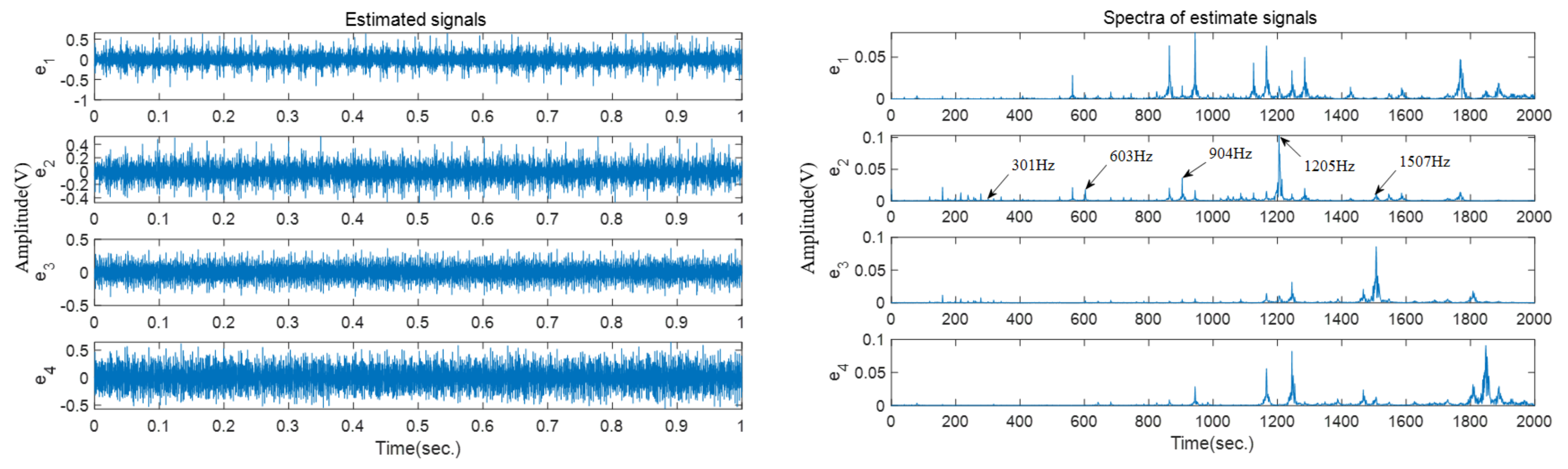
In this case, two vibration signals are collected and presented in Figure 12. The source number is first estimated and then four estimated source signals are obtained based on the improved SCA method. Figure 13 shows the time−domain waveforms and frequency spectra of these four estimated vibration signals. As is shown in the frequency spectra, the harmonic frequencies of the inner race fault can be easily identified in the frequency spectrum of $e_2$; for example, $f_1=302 \mathrm{Hz}\approx f_{bpfi}, f_2=603 \mathrm{Hz}\approx 2f_{bpfi}, f_3=904 \mathrm{Hz}\approx 3f_{bpfi}, f_4=1205 \mathrm{Hz}\approx 4f_{bpfi}, f_5=1507=5f_{bpfi}$.

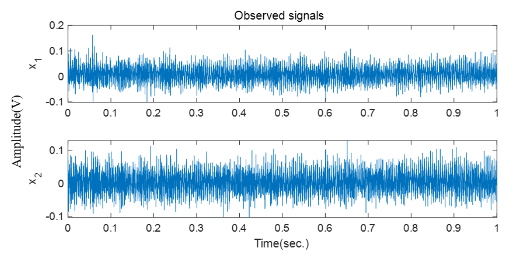
5.2. Outer Race Fault

In this case, two collected vibration signals are used to validate the effectiveness of the proposed approach. Figure 14 shows the time domain waveforms of these signals. Based on the proposed solution, four source signals are recovered, as shown in Figure 15, then the recovered signals are further transformed into the frequency domain. It can be seen that the peak frequency of $e_2$ well match the expected frequency of the outer race fault. The results of the inner and outer race fault amply prove the effectiveness of the proposed bearing fault diagnosis approach.

6. Conclusions

Because the sensor number is restricted by the practical installation position, and the observed signals are often a nonlinear mixture of unknown signals due to the complexity of operating conditions, it is of paramount importance to explore the solution of the nonlinear UBSS problem. In this study, an effective nonlinear UBSS solution based on an EEMD–CC–ATSVD joint approach and improved SCA is presented to diagnose the bearing fault. EEMD is employed to decompose the original observed signals into $m$ sets of IMFs and the CC technique is adopted to screen for the significant IMFs. The retained IMFs and the observed signals are reconstructed into new observed signals, and ATSVD is applied to estimate the source number. The original observed signals are then changed into a time−frequency domain via STFT. Based on the estimated source number, $\widehat{n}$, the frequency data points corresponding to the $\widehat{n}$ peaks of frequency energy sum are picked and clustered into two categories by FCM. The first row of the cluster center matrix is adopted to form the mixing matrix. The L1−norm minimization method is employed to recover the source signals in the time−frequency domain, and then inverse STFT is utilized to obtain the estimated source signals in the time domain. The simulation results prove that the proposed EEMD–CC–ATSVD joint approach can exactly estimate the source number, and the improved SCA can well recover the source signals, in both linear and nonlinear mixed cases. Finally, inner race and outer race fault bench tests are conducted to validate the effectiveness of the proposed method in bearing fault diagnosis.