Article

Integrated Smart Warehouse and Manufacturing Management with Demand Forecasting in Small-Scale Cyclical Industries

1
Department of Industrial and Systems Engineering, The Hong Kong Polytechnic University, Hong Kong, China
2
Department of Supply Chain and Information Management, The Hang Seng University of Hong Kong, Hong Kong, China
3
Division of Business and Hospitality Management, College of Professional and Continuing Education, The Hong Kong Polytechnic University, Hong Kong, China
*
Author to whom correspondence should be addressed.
Machines 2022, 10(6), 472; https://doi.org/10.3390/machines10060472
Submission received: 18 May 2022 / Revised: 3 June 2022 / Accepted: 10 June 2022 / Published: 14 June 2022
(This article belongs to the Special Issue Digital Twin Applications in Smart Manufacturing)

Abstract

:
In the context of the global economic slowdown, demand forecasting, and inventory and production management have long been important topics to the industries. With the support of smart warehouses, big data analytics, and optimization algorithms, enterprises can achieve economies of scale, and balance supply and demand. Smart warehouse and manufacturing management is considered the culmination of recently advanced technologies. It is important to enhance the scalability and extendibility of the industry. Despite many researchers having developed frameworks for smart warehouse and manufacturing management for various fields, most of these models are mainly focused on the logistics of the product and are not generalized to tackle the specific manufacturing problem facing in the cyclical industry. Indeed, the cyclical industry has a key problem: the big risk which high sensitivity poses to the business cycle and economic recession, which is difficult to foresee. Despite many inventory optimization approaches being proposed to optimize the inventory level in the warehouse and facilitate production management, the demand forecasting technique is seldom focused on the cyclic industry. On the other hand, management approaches are usually based on the complex logistics process instead of integrating the inventory level of the stock, which is very crucial to composing smart warehouses and manufacturing. This research study proposed a digital twin framework by integrating the smart warehouse and manufacturing with the roulette genetic algorithm for demand forecasting in the cyclical industry. We also demonstrate how this algorithm is practically implemented for forecasting the demand, sustaining manufacturing optimization, and achieving inventory optimization. We adopted a small-scale textile company case study to demonstrate the proposed digital framework in the warehouse and demonstrate the results of demand forecasting and inventory optimization. Various scenarios were conducted to simulate the results for the digital twin. The proposed digital twin framework and results help manufacturers and logistics companies to improve inventory management. This study has important theoretical and practical significance for the management of the cyclical industry.

1. Introduction

A cyclical industry refers to an industry that follows domestic and foreign economic fluctuations. It is generally believed that industries with high demand income elasticity, such as the consumer goods industry and the durable goods manufacturing industry, are cyclical [1]. Periodic industry enterprises are the main components of the stock market, and changes in the dynamic economic cycle cause the rise and fall of their performance and share prices [2]. In the current global economic slowdown, cyclical enterprises regularly need to adjust their business management strategies and manufacturing capabilities to develop sustainable development. FinTech and e-business are new, innovative approaches which have emerged in the past few years [3]. Sales management, strategic manufacturing management, and inventory management can help businesses realize scale economies, meet the balance of supply and demand, and prevent the demand and order cycle [4].
To help an enterprise have better inventory control, robust demand forecasting methods are essential to developing an algorithm for inventory optimization. There are various ways to forecast product demand, such as the qualitative method, decomposition forecasting, the Box–Jenkins method, and genetic algorithms (GAs), etc. [5,6]. In the past, GAs have been widely used in inventory management. Du and Luo [7] combined the true situation of hospital drug inventory prediction by using GAs and backpropagation neural networks and establishing a system model based on a hospital drug management model. Fakhrzad and Alidoosti [8] employed GAs to make a realistic perishability inventory management system for the location–inventory–routing problem. This strategy is commonly adopted in biomedicine and industry, but there is little literature on enterprise operation. Based on the results from demand forecasting, various techniques are applied for inventory control and optimization. A smart warehouse is considered as the culmination of recent advanced technologies for Industry 4.0, such as 5G, automation, information systems integration, Internet of Things (IoT), blockchain, etc., for improving the supply chain performance of the industry [9]. Those technologies are usually associated with the traceability and trackability of each product item [10] to enhance the visualization of the product data for the customers and industrial practitioners, as well as the innovativeness and reliability [11].
Nevertheless, the development of smart warehouses is usually implemented in a manufacturing management system that uses IoT sensors, radio frequency identification (RFID) technology, etc. [12,13]. Most of the existing researchers are focused on tracking the flow of products and materials [14], rather than considering the optimization of warehouse space, manufacturing capacity, and inventory levels. Weißhuhn and Hoberg [15] propose the adoption of the recent advance of IoT technology in smart replenishment system modelling for household appliances. Lyu and Lin [16] constructed the Zero-Warehousing Smart Manufacturing platform based on IoT-enabled infrastructures. The platform demonstrated the approach for a local construction project from zero-inventory to just-in-time production. Nevertheless, these projects are mainly concentrated on a single project or small-scale project compared with a large-scale product warehouse, which consists of a large area, many employees, transportation facilities, equipment, and autonomous robots, etc. [17]. There is also a lack of optimization approaches for adjusting inventory levels and manufacturing capacities in smart warehouses.
A smart warehouse management system works in conjunction with the supply chain, stock level, manufacturing capacity, and demand forecasting to decide the necessary stock replenishment. Despite the various product replenishment approaches which have been proposed [18], there is a lack of publications that consider smart warehouse management based on inventory optimization and propose an implementation framework using the digital twin approach to integrate demand forecasting to provide feedback, facilitating actual smart industrial management. Indeed, the cyclic industries are industries that have a high demand for effective management and are integrated into actual manufacturing scenarios. As such, this article aims to fill in the gaps that propose the implementation of a digital twin framework for smart warehouses, particularly concerning the optimization of the inventory level according to the demand forecasting results. We suggest that the roulette selection genetic algorithm should be applied in the cyclic industry for demand forecasting to achieve inventory optimization. The company studied in this paper is a small-scale textile enterprise. Roulette wheel selection is used to ensure that individuals or nodes with better adaptability and target functions have a greater chance of being selected, which is particularly essential in the estimation of the cyclic industry that is largely affected by the economic recession and trend [19].
Although it is challenging to perform an actual implementation and data collection in real smart manufacturing and warehouses for results validation, this study presents a twofold academic contribution. Firstly, we propose a practical framework for implementing a digital twin in the smart warehouse by considering the manufacturing infrastructure, data integration, demand forecasting, and inventory optimization throughout the sophisticated logistics process. Secondly, a roulette wheel selection based on the genetic algorithm is proposed for application to demand forecasting to achieve an optimum stock level. The approach is shown to be adaptable to the cyclical industry. In particular, digital twin frameworks enable these various simulation settings to be performed multiple times, achieving desirable results that are adaptable to real cases in a small-scale textile enterprise. The paper has important impact not only on the development of digital twins or smart warehouses for small-scale industries, but also in demonstrating how inventory forecasting is an essential part of future smart warehouses.

2. Literature Review

2.1. Digital Twins and Smart Warehouse Management

The digital twin refers to “an integrated multi-physics, multiscale, probabilistic simulation of an as-built vehicle or system that uses the best available physical models, sensor updates, fleet history, etc. to mirror the life of its corresponding flying twin” [20]. The digital twin is a virtual experiment that simulates a physical object or process over a period of time. Liu et al. [21] conducted a critical review of 240 research papers to highlight the clear features of a digital twin system. The main features of a digital twin system are integrated simulation, real-time control and optimization, dynamic reflection, mapping, and bidirectionality. Currently, the adoption of digital twin technology has been enlarged from the operation to the design of a manufacturing system [22,23]. Indeed, these technology tools can help the warehousing industry to maximize its manufacturing capacity and reduce supply chain lead times to attain lean, flexible, and intelligent production and supply chain management [24]. Digital twin technology establishes a close alignment between the virtual environment and the real world. The technology fosters the development of remote monitor systems and components, performs digital simulation to test and predict changes in the process of hypothetical scenarios, and further analyzes the performance of operations that drive product innovation and the management of delivery time in logistics management [25,26].
Nowadays, the digital twin is being widely used to study various manufacturing production operating systems and supply chain warehousing systems, and to measure the overall performance of organizations [27]. The approach can virtually represent the dynamic characteristics of the logistics model in terms of function and cost and can also accurately capture the complex behavior and changes in the model. The simulated model can be revised through data collected from the IoT devices, thereby improving the performance of the system, and increasing cost effectiveness [28]. For example, Kim [29] set up the optimal warehouse interception and pick-up time based on customer order response capabilities and priority-based job scheduling, using a streamlined operating model to help warehouse managers make optimal decisions. Sahay and Ierapetritou [30] pioneered a hybrid simulation modelling approach by combining the iterative model and the simulation model. The optimal allocation of resources can be determined under multiple problems and constraints, such as the determination of the optimal inventory, performed regularly [31,32]. The characteristics of the geographic information system in the simulation modelling software will assist in planning the optimal positioning of the distribution center and the optimization of transportation routes, product routes, and supply chains in the smart warehouse. After completing a validated digital twin model, the model should include interrupted parameters and respective solutions to explore different scenarios. These models are retrieved separately to build a reinforcement learning algorithm and create a prescriptive analysis platform as the basis of the logistics 4.0 decision-support system. Despite the digital twin technology being widely studied for smart warehouses, most of the approaches lack the integration of the demand forecasting algorithm which is essential to optimize the logistics process. Loaiza and Cloutier [33] also criticized the fact that the digital twin approach mainly changes physical spaces to virtual spaces. Such digital transformation leads to unexpected problems being created and influences a manufacturing system’s lifecycle. Nevertheless, numerous logistics firms may face the challenges of time and costs to develop and implement digital twin technology. In terms of the subsystem level, there is no connectivity or integration of the digital twin components or other devices in the system. Regarding the system level, there are incorrect digital twin models and an unclear definition of a manufacturing system. Concerning the super-system level, there is a deficiency of connection between systems to avoid a supply chain interruption.

2.2. Demand Forecasting and Inventory Optimization

Demand forecasting can be performed based on qualitative and quantitative methods. The qualitative method relies on the investigator’s knowledge of the research topic or the experts’ subjective judgment. Although qualitative forecasting may be based on not easy-to-quantify factors, it is frequently adopted in all kinds of demand forecasts. Four judgmental techniques are used: independent judgment, committee judgment, salesforce estimates, and executive opinion juries [34].
Quantitative methods use historical data and mathematical equations to forecast demand. Time–series methods and quantitative analysis methods based on genetic algorithms are often used to predict demand. A time–series approach can be used to investigate trends and seasonal and cyclical factors that can affect a particular product’s demand [35]. There are several time–series methods, including naive or random walk, moving to average, exponential smoothing, decomposition, and ARIMA [36]. The strengths and weakness of the moving average, simple exponential, Holt two-parameter, and Holt–Winters methods were detailed by Chase [34]. To sort out the similarities and differences between these four methods more efficiently, Table 1 summarizes and compares various time–series methods.
GA is a method of simulating evolution and natural selection to determine optimal solutions to a problem. After selection, crossover, and mutation, a group of individuals evolves and becomes the result we obtained. The fitness function determines how individuals multiply after the selection process [37]. The GA can be used to forecast demand effectively, and the combination of multiple models improves accuracy. For example, He and Chang [38] developed a combined prediction model to predict regional logistics demand. Techniques combined with GA include support vector regression (SVR) [39,40], fuzzy set theory [41], and neural networks (NN) [42]. In addition to forecasting demand, Chen and Sarker [43] predicted the number of tourists in the tourism industry by combining SVR with adaptive function and seasonal index adjustment. GA also plays a prominent role as a market forecasting tool in the financial field [40].
GA has been widely used in research to predict inventory and improve inventory management. Isen and Boran [44] proposed a hybrid model generated byGA, fuzzy C-means (FCM), and adaptive neuro-fuzzy reasoning system (ANFIS) for inventory classification, which has great application value. Bhunia and Kundu [45] use a hybrid tournament genetic algorithm (TGA) to solve partial backlogged shortages where a deterioration rate of items was investigated. Some researchers have solved the routing problem using inventory control [46]. Azadeh and Elahi [47] were the first to use GA to solve perishable goods inventory management problems. Furthermore, Hiassat and Diabat [48] proposed a location–inventory–path model for perishable products and made an outstanding contribution to inventory management by using GAs to determine the number and location of required warehouses. GA is one of the effective approaches for demand forecasting, while various assumptions and constraints have to be designed to optimize the level of inventory.

3. Methodology

In this section, we present the methodology for the development of our demand forecasting algorithm. The development is divided into three main sections, including data acquisition and preparation, roulette genetic algorithm for demand forecasting, and the inventory optimization approach. In this paper, we adopted a small-scale textile industry as the case study.

3.1. Data Acquisition and Preparation

The data were collected from the record of the case study company database. The database included the sales record, inventory records, product categories, and price lists from the last two years. The database consisted of intensive raw data including over a hundred product categories, everyday sales records for each product, selling prices, etc. To ensure the data were valid, unified, and complete, the data cleaning processes based on the guideline were performed [49] to remove errors, irrelevant data, and inconsistencies from the dataset. The knowledge discovery and data mining (KDD) process were used to clean the dataset to make it more easily readable and understandable for further analyses. The KDD process is illustrated in Figure 1.

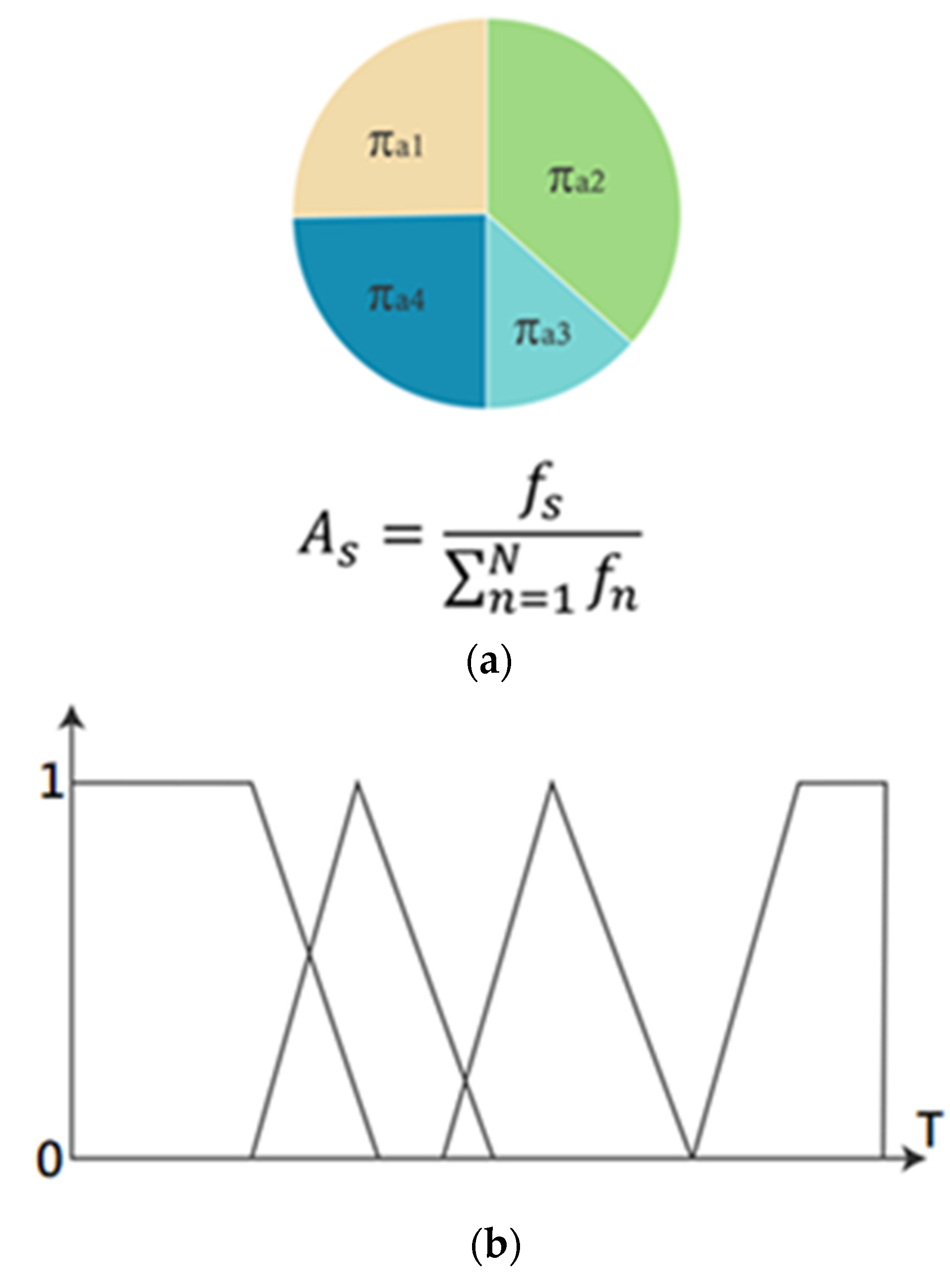
3.2. Roulette Genetic Algorithm

To perform the inventory optimization, we suggested an algorithm be produced for forecasting the demand of the customers in the first step. The genetic algorithm (GA) was proposed for demand forecasting. To adapt to the change in demand for the cyclic industry, roulette selection was suggested to generate the seed for the forecasting. The integrated roulette genetic algorithm was proposed for application in forecasting the demand, and it was demonstrated in the case study company.
In the GA, Chodak and Kwaśnicki [50] found that factors that affect demand function change with each company. The simple form of the product or service demand function, D, can be derived, as in Equation (1):
D = M ( t ) p e
where the price is denoted by p, time is denoted by t, price elasticity is denoted by e, and M(t) represents the trend and the periodicity of demand with time.
Due to the seasonal demand nature of the cyclical industry, the demand function can be derived, as in Equation (2):
D = C + B × t + A × s i n ( ω × t + φ ) p e
where D is the monthly product demand of a company, t refers to the number of months, and A refers to the amplitude that is equal to the maximum and minimum sales quantities. B is the trend factor that represents increasing or decreasing sales, ω refers to the frequency that means the periodicity of the demand curve in terms of π, and the demand function can be represented as a sine curve. Hence, 2π can indicate one cycle of the sine wave. Horizontal offset (φ) refers to the demand function shift along with the horizontal level, which is represented in the range from 0π to 2π, while vertical offset (C) refers to the demand function shift vertically, which is represented in the range from 0 to the maximum sales value in the input data. Finally, P (price) is a weighted average price, and e represents price elasticity.
After defining the demand function, each individual has six parameters encoded in chromosome form to define the fitness function, which measures the difference between the input data set and the GA’s data. The GA searches for the optimal value in the parameter space in terms of size steps in the path search by acting on genetic operators on bit strings. The first step, the fitness function, is defined in Equation (3):
F = t | D t { C + B × t + A × s i n ( ω × t + φ ) p e } | .
The six parameters (C, B, A, ω, φ, and e) represent six segments of one chromosome [50]. Each chromosome will be 60 bits in length, and each parameter’s length will be 10 bits [50]. Each 10-bit gene can represent 210 possible values for a range of 0–1024. The binary coding represents numerical values and non-numerical values, such as options and colors [51]. However, the chromosome only represents numerical values in this study.
The next step of the GA is to estimate each of the parameters to minimize the fitness function. To select the individuals to have further crossover and mutation in GA, a revised roulette wheel method [52,53] was adopted. The cumulative fitness function of all individuals is a whole wheel. Each individual has a different weight on the wheel, and this weight is proportional to the individual’s suitability. Figure 2 shows the revised model of the roulette method concept, where each sector has different fitness. A larger area of the roulette wheel has a higher chance of being selected (Figure 2a). The area of the roulette wheel is determined based on the fitness value of the chromosome, which can be calculated by Equation (4):
A s = f s n = 1 N f n × 100
where fs is the fitness value of the chromosome, s. N is the total number of chromosomes. The slices which represent each chromosome have a total size equal to 100% of the roulette wheel. The crossover and mutation then take place and two chromosomes exchange the bit string through a single-point crossover. A mutation rate is decided to determine whether a gene in the chromosome will mutate or not. A bit in the chromosome will then take its inverse, from 0 to 1 or vice versa, based on the fuzzy rules, as illustrated in Figure 2b.
The fitness function of the analyzed product was prepared in the MATLAB script. The upper boundaries and lower boundaries of the six parameters (C, B, A, ω φ, and e) were predefined. The constraints of the GA optimization were defined to identify optimal value. The stopping criteria of the GA were defined as follows:
  • The maximum number of generations is exceeded;
  • Or, the average change in the fitness value is less than the other options.
The GA stops when either of the two stopping criteria is satisfied. The process is repeated 10 times to find the lowest fitness value for the GA. The lower value of the fitness function indicates the higher fitness of the prediction in the real data set. To analyze the robustness of the forecasting algorithm in the forecasting of the cyclical industry, the dataset was separated into three types of prediction periods for forecasting and compared based on the three prediction period settings. Table 2 illustrates the conceptual diagram of how the 20 months of sales records were divided into the three prediction periods, named type I, type II, and type III (Figure 3). Type I represents the prediction of the last 4 months based on the previous 16 months. For type II, the last 2 months’ predictions are based on 8 months’ data, while only 6 months are used for the type III prediction. The prediction of the preceding months is used to predict the following 2 months; this continues for all the following predictions.

3.3. Inventory Optimization

In this paper, we proposed the inventory optimization models for calculation including the safety stock statistical model and the dynamic safety stock model. To achieve inventory optimization, the level of safety stock should be kept at an appropriate level [54]. The safety stock statistical model calculation can be used when the replenishment time is confirmed and stock consumption is random [55,56]. The safety stock equation is as follows:
S a f e t y s t o c k = Z × ( L T T × σ D 2 ) + ( σ L T × D a v g ) 2 .
The service factor (Z-score) is represented by Z. The standard deviation of demand is represented by σD, where the lead time standard deviation is represented by σLT. The lead time is labelled LT, and T represents the time that is used for the standard deviation of demand. The last variable, Davg, refers to average demand.
However, as the company does not record lead time, the variable L T T is simplified to average lead time or ALT. In doing so, we proposed the dynamic safety stock model which is calculated using the following equation:
S a f e t y s t o c k = Z × ( A L T × σ D 2 ) + ( σ L T × D a v g ) 2 .
On the other hand, the changing safety stock model will be combined to calculate safety stock and inventory. Ferbar Tratar [57] suggested a method to minimize the safety stock of a seasonal product, and the equations are as follows:
σ = D e v i a t i o n 2 N 1
S a f e t y s t o c k = Z × L T × σ 2
where the deviation is the prediction difference from real sales, and N refers to the number of observations. LT refers here to the average lead time. The variables in the Equations were calculated using Excel. The monthly inventory prediction can be obtained by adding the average demand and safety stock.

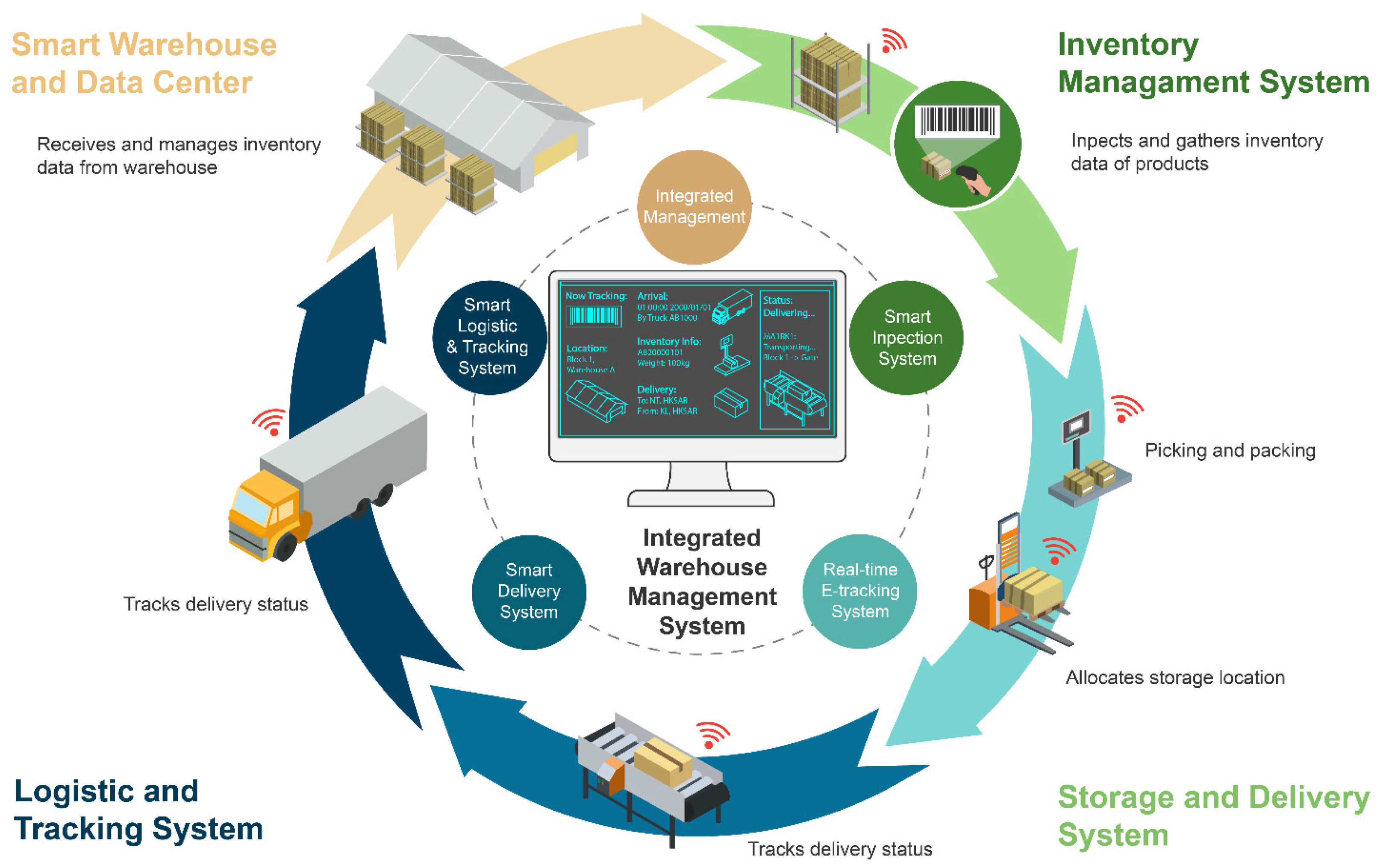
3.4. Proposed Digital Twin in Smart Warehouse
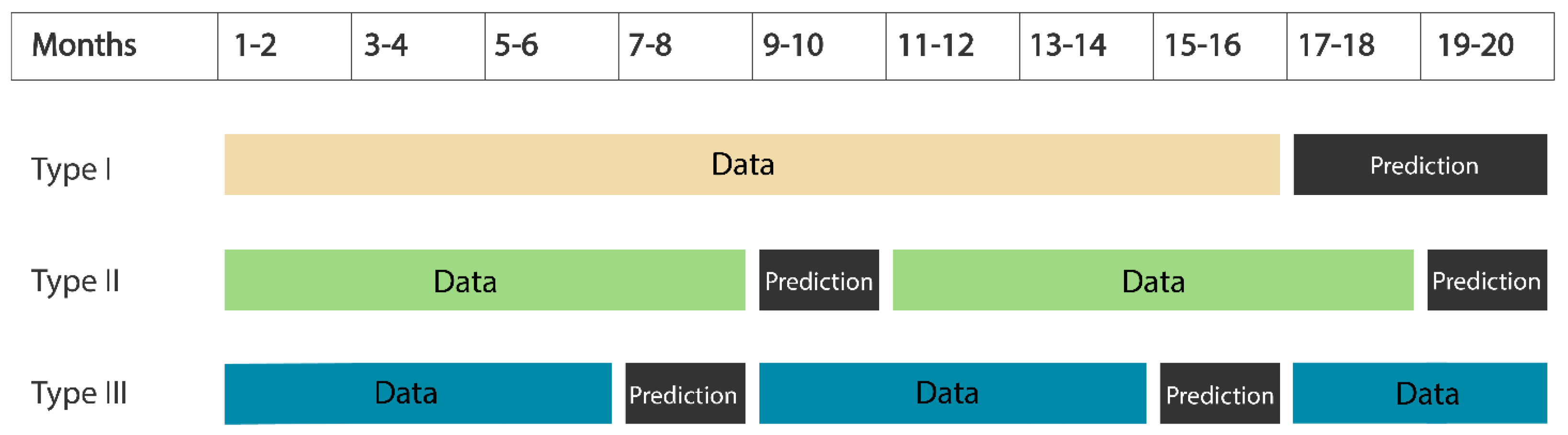
Figure 4 illustrates the proposed digital twin model in the smart warehouse for the small-scale cyclical industry. The proposed integrated digital twin smart warehouse management system has two layers including the physical layer and virtual layer. The virtual layer in the digital twin composes of the smart logistics and tracking system, integrated management system, smart perception system, real-time e-tracking system, and smart delivery system. The layer is integrated with the physical layer through the IoT devices and enterprise information systems that form the digital twin network.
At the physical layer, the smart warehouse and data center receives and manages inventory data from the warehouse. In the smart warehouse, the order is automatically received, and then the system confirms whether the product is in stock. Then, the pick-up list is sent to the robot cart, the ordered products are put into the container, and then they are handed over to the workers for the next step. The inventory management system summarizes and gathers products inventory data and demand forecasting information in the virtual layer to perform inventory management, with in storage and out of storage types, and with a query as the main application type to establish the corresponding transaction processing, so that the quantity of goods inventory is controlled in the best state. In the management system, the revised model of the fuzzy roulette selection method for demand forecasting was integrated with the inventory optimization approach to deal with the complex variation of the inventory record. The inventory record is dynamically updated to provide data to the following suppliers and manufacturers, as well as the procurement manager to control the supplies and inventory to a certain optimized level. As such, the digital twin framework can be designed to deal with the deviation in real demand and the simulated inventory optimization under the actual situation.
The storage delivery system uses data to pick, package, and redistribute the storage location, and finally query and observe and track the delivery status through the logistics tracking system, which was originally a means used by logistics enterprises to track the flow of internal goods. The tracking system determines the time of each transportation, sorting, transit, and distribution, and can even be accurate to the exact time in each link that constitutes the integrated digital twin smart warehouse management framework.

4. Results

In this section, the experimental results are illustrated in four key sections. In the beginning, the initial GA parameter settings are defined based on the test case scenario. Then, the prediction results are illustrated, and different types of prediction are compared to determine better settings of the demand forecasting approach, followed by the results for optimizing the inventory level. Lastly, the framework for implementing the smart warehouse in the case study company is elaborated.

4.1. Roulette GA Settings

A roulette GA was applied to predict the product demand of the studied company. A product item with the highest number of recorded transaction times was selected as it provides a larger sample size to exhibit the sales forecast procedure. We performed analysis of 20 months of data to illustrate the results. Different parameters were initially set for the GA, including the generation size and crossover probability, and the mutation rate influences the calculation speed. The parameter settings for GA optimization were defined as follows:
  • Population size: 1000.
  • Constraint-dependent mutation function.
  • Constraint-dependent crossover function.
  • Crossover fraction: 0.2.
  • Stopping criteria generation: 1000.

4.2. Demand Forecasting

In this section, the prediction period of types I, II, and III and implemented and compared to determine the error between different types of prediction periods for the proposed algorithm. The average error in the quantity, root mean square error (RMSE), and the percentage error was used to determine the accuracy of the approach. The results are summarized in Table 2.
In the beginning, the prediction period type I was used. In this period, the first 16 months of historical data were used to predict the last 4 months of demand. The prediction results found that the sum of the errors was 1261.8 units, and the average error was 78.9 units. The percentage error of the sales forecast was 19.59%. The RMSE was 120.72, which indicated that the GA prediction model was far from the real data. In the forecasting of the prediction period, the prediction curve is similar to the historical data. However, the second year’s prediction tends to smooth the amplitude, and the curve became flattened and was less similar to the historical sales record than the first year.
Then, prediction type II separated the data into two years for forecasting. The first eight months of historical data in each year were used to predict the last two months of demand in the same year. The integration of the entire sales forecast was created by accumulating the prediction results. According to the results predicted, the sum of the errors was 316.1 units, and the average error was 56.80 units. The percentage error of the sales forecast was 22.18%. The RMSE was 91.76, which was moderate and showed that the prediction was close to the historical data. The type III prediction period performed prediction based on the data from the first 4 months. The results showed that the RMSE of the sales forecast was 103.98 and the percentage error was 10.62%.
Table 2 summarizes the prediction error of the demand forecasting between types I, II, and III of the forecasting periods. The results revealed that these three types of prediction periods showed a similar result in terms of RMSE and percentage error which is important to the cyclical industries. However, a longer period of historical data is believed to increase the forecasting accuracy due to the cyclical feature of this industry as the results have shown that Type I forecasting can effectively forecast the sharp changes in the demand during a sudden economic recession as presented in the historical data. This approach effectively facilitates the cyclical industry to estimate peak season demand, thus it is useful for developing sales strategies in the future.

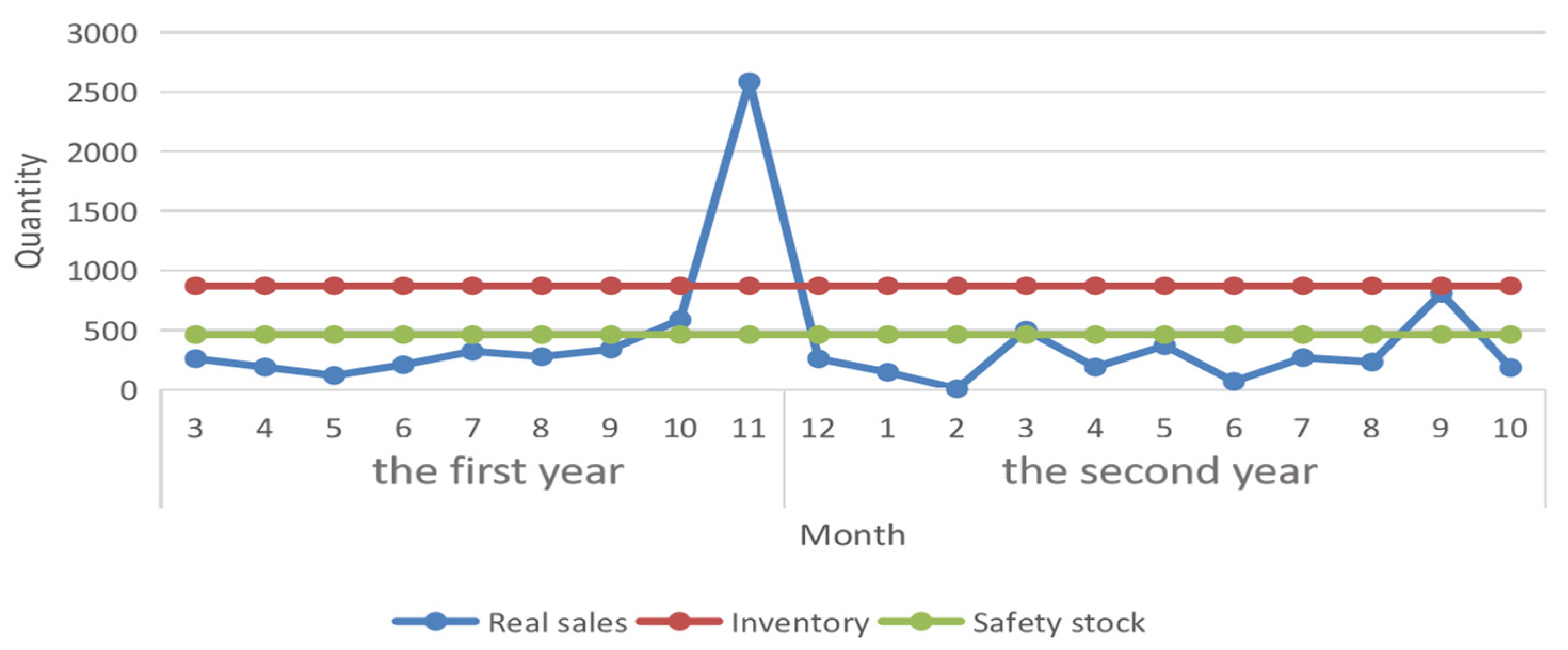
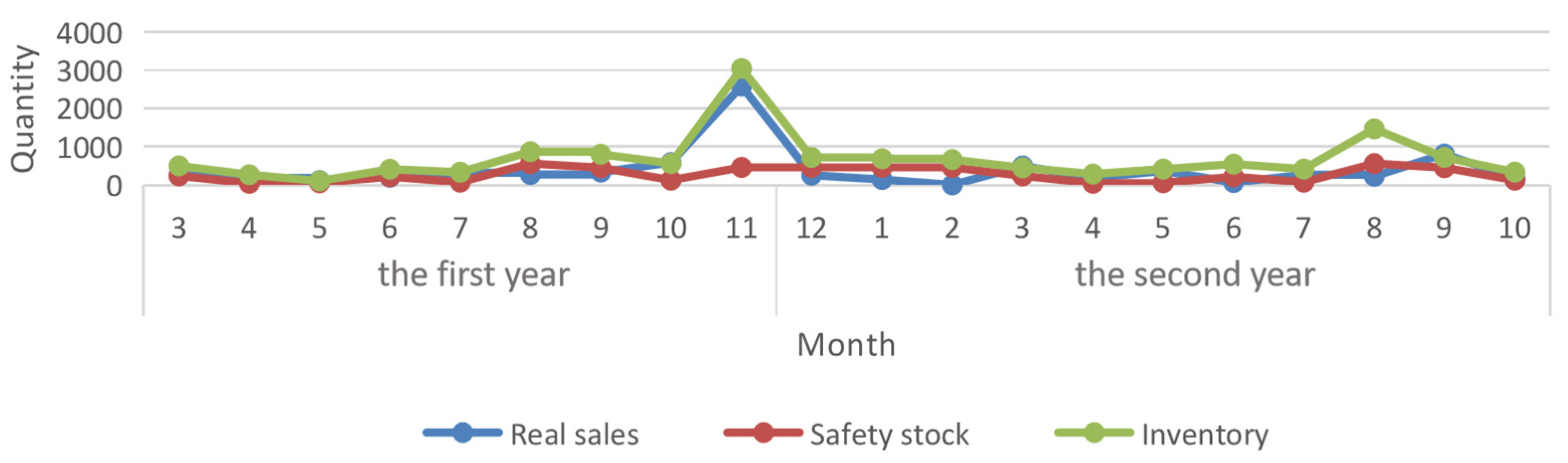
4.3. Inventory Optimization

This section proposed the approaches for inventory optimization, we proposed two approaches for optimizing the inventory including the safety stock statistical model and dynamic safety stock model. The approaches were compared to determine an appropriate safety stock approach for the cyclical industry.

4.3.1. Safety Stock Statistical Model

In this model, Equation (5) was used to calculate safety stock. The service factor (Z), lead time (ALT), and standard deviation of the lead time (σLT) were obtained from the assumption due to the lack of readily available first-hand data from the company. The function of Z in the safety stock calculation was used as a factor and multiplied with the standard deviation to ensure the inventory could fulfil company service levels. ABC analysis is one method that fosters companies to determine optimum service levels [50]. Class A product contributes the highest 20% of company revenue; Class B contributes around 20–30%; and Class C contributes 50–60%. The studied product, cotton twill, is a Class A product. The service level of Class A products should be between 96% and 98%. The service level of cotton twill is defined at 98% and is converted to a service factor, which is 1.75 (Z). The inventory level is predicted monthly. The lead time is converted from 7 days to 0.23 months (T). The standard deviation of the assumed monthly lead time (σLT) is 0.05. The 16-month predicted demand figure is equal to the sales forecast quantity.
The monthly demand for the study period was obtained from historical and predicted data. The predicted demand covers 4 months of the second year (the forecast result uses prediction type I). The historical sales record of the remaining 12 months was used as the monthly demand in the safety stock calculation. The average demand (Davg) was equal to 408.2 units. The standard deviation of the demand (σD) was rounded to three decimal places for 549.082. The safety stock was calculated according to and equaled 462.54 units. Thus, there should be 463 units of safety stock in the warehouse. The monthly inventory was predicted by adding the average demand and safety stock, which was 872 units.
Figure 5 shows that the inventory of the company was prepared using the safety stock statistical model. The safety stock level is higher than 18 months of real demand. Only the demand in March and September of the second year was greater than the safety stock level. Safety stock was overestimated in non-peak months. This overestimation becomes more severe in predicting inventory level because the high seasonal demand in November of the first year has induced many effects on the standard deviation of demand.

4.3.2. Dynamic Safety Stock Level Model

Then, a dynamic safety stock level w using Equations (6) and (7) was adopted to reduce the influence of high seasonality [58]. However, this approach does not apply to a non-repeated month in the observations. Part of the standard deviation equation in this model was calculated by dividing the number of observations by minus one. The historical data for the product item has four non-repeated months: January and February of the first year and November and December of the second year. For these months, the monthly safety stock is equal to the value determined by the safety stock statistical model (463 units). Each of the remaining eight months has two observations. The monthly inventory was predicted by adding monthly predicted demand and monthly safety stock. The results calculated using the changing safety stock level model are illustrated in Figure 6.

5. Conclusions

In this study, a digital twin model for the smart warehouse was proposed. The smart warehouse was suggested to integrate with demand forecasting and inventory optimization for manufacturing management. The digital twin model enables the demand forecasting results to be simulated under prediction periods as well as using different inventory optimization models. The digital twin model can be adaptable to the change in the forecasting and inventory results which is particularly important in the cyclical industry that needs to deal with the sudden change of demand during the economic progression as well as the demand for seasonal products. Through demand forecasting, sales patterns can be determined and predicted. The methods proposed in this study can generate sales patterns, demand predictions, and inventory optimization, and these data are useful for small- and medium-sized enterprises to understand marketing trends more easily. The seasonality and trends can be observed using graphical representations of demand predictions. The data facilitates the company to establish a business plan and arrange the supply chain to deliver customers’ services on time. Furthermore, the risk of losing a potential customer can be lowered by preparing adequate safety stock.
This paper provides evidence to help cyclical companies perform inventory management. The comparison of stock minimization and the prediction information is also useful to improve their inventory management. Some of the components of inventory management were fulfilled in this study, and companies can use them to improve inventory management time in the long term. More resources should be invested in manufacturing management and product demand analysis for companies. Finally, other cyclical enterprises can use the information gleaned from this research as inventory management evidence and perform product demand predictions to capture market trends and align with manufacturing capacity.
Nevertheless, there are two limitations to the project. There are difficulties in preparing data to perform precise demand forecasts. There is a high variation in product choice, because each product has a different choice of colour and size. Additionally, we had incomplete and outdated data. The second limitation is that the demand function used is less sensitive to seasonality products. The inventory prediction method proposed in the study is more suitable for a product that has less seasonality. Although some of the textile products are seasonal, the company can still use the method on their product to gather the initial demand prediction. The nonseasonal development of the textile company can obtain a high accuracy of the demand forecast. For future research in this area, we recommend the following. The genetic algorithm and artificial intelligence neural network can be combined to improve the accuracy of inventory prediction. The methods can also be implemented in other industries for comparison, which may also be helpful to enlarge the database for better accuracy in demand forecasting and thus inventory optimization.

Author Contributions

Y.-M.T. and S.-Y.T. collected and analysed the data; Y.-M.T. and S.-Y.T. wrote the manuscript. G.T.S.H. and Y.-Y.L. edited and revised the paper. All authors have read and agreed to the published version of the manuscript.

Funding

This project is supported partially by the Funding for Strategic Plan Initiatives to Expand Research Elements in the Undergraduate Curriculum 2020-22, the Hong Kong Polytechnic University (Ref.: SPF20-22/ISE) and matching grant from the University Grants Committee of the Hong Kong (RMGS Project No. 700007).

Institutional Review Board Statement

Not applicable.

Informed Consent Statement

Not applicable.

Data Availability Statement

Not applicable.

Acknowledgments

The authors would like to thank the support of the Hong Kong Polytechnic University and the Big Data Intelligence Centre in The Hang Seng University of Hong Kong.

Conflicts of Interest

The authors declare no conflict of interest.

References

  1. He, Y.; Lin, B. Time-varying effects of cyclical fluctuations in China’s energy industry on the macro economy and carbon emissions. Energy 2018, 155, 1102–1112. [Google Scholar] [CrossRef]
  2. Drobetz, W.; Menzel, C.; Schröder, H. Systematic risk behavior in cyclical industries: The case of shipping. Transp. Res. Part E Logist. Transp. Rev. 2016, 88, 129–145. [Google Scholar] [CrossRef]
  3. Tang, Y.; Chau, K.; Hong, L.; Ip, Y.; Yan, W. Financial Innovation in Digital Payment with WeChat towards Electronic Business Success. J. Theor. Appl. Electron. Commer. Res. 2021, 16, 1844–1861. [Google Scholar] [CrossRef]
  4. Ganesha, H.R.; Aithal, P. Integrated Inventory Management Control Framework. Int. J. Manag. Technol. Soc. Sci. IJMTS 2020, 5, 147–157. [Google Scholar] [CrossRef]
  5. He, Z.; Jiang, W. A new belief Markov chain model and its application in inventory prediction. Int. J. Prod. Res. 2018, 56, 2800–2817. [Google Scholar] [CrossRef] [Green Version]
  6. Talib, F.; Asjad, M.; Attri, R.; Siddiquee, A.N.; Khan, Z.A. A road map for the implementation of integrated JIT-lean practices in Indian manufacturing industries using the best-worst method approach. J. Ind. Prod. Eng. 2020, 37, 275–291. [Google Scholar] [CrossRef]
  7. Du, M.; Luo, J.; Wang, S.; Liu, S. Genetic algorithm combined with BP neural network in hospital drug inventory management system. Neural Comput. Appl. 2020, 32, 1981–1994. [Google Scholar] [CrossRef]
  8. Fakhrzad, B.M.; Alidoosti, Z. A realistic perish ability inventory management for location-inventory-routing problem based on Genetic Algorithm. J. Ind. Eng. Manag. Stud. 2018, 5, 106–121. [Google Scholar]
  9. Chau, K.-Y.; Tang, Y.M.; Liu, X.; Ip, Y.-K.; Tao, Y. Investigation of critical success factors for improving supply chain quality management in manufacturing. Enterp. Inf. Syst. 2021, 15, 1418–1437. [Google Scholar] [CrossRef]
  10. Ho, G.; Tang, Y.M.; Tsang, K.Y.; Tang, V.; Chau, K.Y. A blockchain-based system to enhance aircraft parts traceability and trackability for inventory management. Expert Syst. Appl. 2021, 179, 115101. [Google Scholar] [CrossRef]
  11. Yung, K.L.; Ho, G.T.S.; Tang, Y.M.; Ip, W.H. Inventory classification system in space mission component replenishment using multi-attribute fuzzy ABC classification. Ind. Manag. Data Syst. 2021, 121, 637–656. [Google Scholar] [CrossRef]
  12. Tejesh, S.B.S.; Neeraja, S. Warehouse inventory management system using IoT and open source framework. Alex. Eng. J. 2018, 57, 3817–3823. [Google Scholar] [CrossRef]
  13. Binos, T.; Bruno, V.; Adamopoulos, A. Intelligent agent based framework to augment warehouse management systems for dynamic demand environments. Australas. J. Inf. Syst. 2021, 25, 1–25. [Google Scholar] [CrossRef]
  14. Tang, Y.M.; Chau, K.Y.; Xu, D.; Liu, X. Consumer perceptions to support IoT based smart parcel locker logistics in China. J. Retail. Consum. Serv. 2021, 62, 102659. [Google Scholar] [CrossRef]
  15. Weißhuhn, S.; Hoberg, K. Designing smart replenishment systems: Internet-of-Things technology for vendor-managed inventory at end consumers. Eur. J. Oper. Res. 2021, 295, 949–964. [Google Scholar] [CrossRef]
  16. Lyu, Z.; Lin, P.; Guo, D.; Huang, G.Q. Towards zero-warehousing smart manufacturing from zero-inventory just-in-time production. Robot. Comput. -Integr. Manuf. 2020, 64, 101932. [Google Scholar] [CrossRef]
  17. van Geest, M.; Tekinerdogan, B.; Catal, C. Design of a reference architecture for developing smart warehouses in industry 4.0. Comput. Ind. 2021, 124, 103343. [Google Scholar] [CrossRef]
  18. Yung, K.-L.; Tang, Y.-M.; Ip, W.-H.; Kuo, W.-T. A systematic review of product design for space instrument innovation, reliability, and manufacturing. Machines 2021, 9, 244. [Google Scholar] [CrossRef]
  19. Tang, Y.; Chau, K.-Y.; Li, W.; Wan, T. Forecasting economic recession through share price in the logistics industry with artificial intelligence (AI). Computation 2020, 8, 70. [Google Scholar] [CrossRef]
  20. Qi, Q.; Tao, F.; Hu, T.; Answer, N.; Liu, A.; Wei, Y.; Wang, L.; Nee, A.Y.C. Enabling technologies and tools for digital twin. J. Manuf. Syst. 2021, 58, 3–21. [Google Scholar] [CrossRef]
  21. Liu, M.; Fang, S.; Dong, H.; Xu, C. Review of digital twin about concepts, technologies, and industrial applications. J. Manuf. Syst. 2021, 58, 341–361. [Google Scholar] [CrossRef]
  22. Liu, Q.; Leng, J.; Yan, D.; Zhang, D.; Wei, L.; Yu, A.; Zhao, R.; Zhang, H.; Chen, X. Digital twin-based designing of the configuration, motion, control, and optimization model of a flow-type smart manufacturing system. J. Manuf. Syst. 2021, 58, 52–64. [Google Scholar] [CrossRef]
  23. Hu, F.; Qiu, X.; Jing, G.; Tang, J.; Zhu, Y. Digital twin-based decision making paradigm of raise boring method. J. Intell. Manuf. 2022. [Google Scholar] [CrossRef]
  24. Leng, J.; Yan, D.; Liu, Q.; Zhang, H.; Zhao, G.; Wei, L.; Zhang, D.; Yu, A.; Chen, X. Digital twin-driven joint optimisation of packing and storage assignment in large-scale automated high-rise warehouse product-service system. Int. J. Comput. Integr. Manuf. 2021, 34, 783–800. [Google Scholar] [CrossRef]
  25. Ivanov, D.; Dolgui, A. A digital supply chain twin for managing the disruption risks and resilience in the era of Industry 4.0. Prod. Plan. Control. 2020, 32, 775–788. [Google Scholar] [CrossRef]
  26. Mittal, S.; Tolk, A.; Pyles, A.; Van Balen, N.; Bergollo, K. Digital twin modeling, co-simulation and cyber use-case inclusion methodology for IoT systems. In Proceedings of the 2019 Winter Simulation Conference (WSC), National Harbor, MD, USA, 8–11 December 2019; IEEE: New York, NY, USA, 2019. [Google Scholar]
  27. Abideen, A.; Mohamad, F.B. Improving the performance of a Malaysian pharmaceutical warehouse supply chain by integrating value stream mapping and discrete event simulation. J. Model. Manag. 2020, 16, 70–102. [Google Scholar] [CrossRef]
  28. Ashrafian, A.; Pettersen, O.-G.; Kuntze, K.N.; Franke, J.; Alfnes, E.; Henriksen, K.F.; Spone, J. Full-scale discrete event simulation of an automated modular conveyor system for warehouse logistics. In Proceedings of the IFIP International Conference on Advances in Production Management Systems, Austin, TX, USA, 1–5 September 2019; Springer: New York, NY, USA, 2019. [Google Scholar]
  29. Kim, T.Y. Improving warehouse responsiveness by job priority management: A European distribution centre field study. Comput. Ind. Eng. 2020, 139, 105564. [Google Scholar] [CrossRef]
  30. Sahay, N.; Ierapetritou, M. Supply chain management using an optimization driven simulation approach. AIChE J. 2013, 59, 4612–4626. [Google Scholar] [CrossRef]
  31. Fernández-Caramés, T.M.; Blanco-Novoa, O.; Froiz-Míguez, I.; Fraga-Lamas, P. Towards an autonomous industry 4.0 warehouse: A UAV and blockchain-based system for inventory and traceability applications in big data-driven supply chain management. Sensors 2019, 19, 2394. [Google Scholar] [CrossRef] [Green Version]
  32. Yang, M. Using data driven simulation to build inventory model. In Proceedings of the 2008 Winter Simulation Conference, Miami, FL, USA, 7–10 December 2008; IEEE: New York, NY, USA, 2008. [Google Scholar]
  33. Loaiza, J.H.; Cloutier, R.J. Analyzing the implementation of a digital twin manufacturing system: Using a systems thinking approach. Systems 2022, 10, 22. [Google Scholar] [CrossRef]
  34. Chase, C.W. Demand-Driven Forecasting: A Structured Approach to Forecasting; John Wiley & Sons: Hoboken, NJ, USA, 2013. [Google Scholar]
  35. Darmanyan, A.; Rogachev, A. Modeling and forecasting seasonal and cyclical events using retrospective data. E3S Web Conf. 2020, 217, 06007. [Google Scholar] [CrossRef]
  36. Box, G.E.; Jenkins, G.M.; Reinsel, G.C. Time Series Analysis: Forecasting and Control; John Wiley & Sons: Hoboken, NJ, USA, 2015. [Google Scholar]
  37. Michalewicz, Z. Genetic Algorithms + Data Structures = Evolution Programs; Springer Science & Business Media: Berlin/Heidelberg, Germany, 2013. [Google Scholar]
  38. He, F.-B.; Chang, J. Combined forecasting of regional logistics demand optimized by genetic algorithm. Grey Syst. Theory Appl. 2014, 4, 221–231. [Google Scholar] [CrossRef]
  39. Chen, R.; Liang, C.-Y.; Hong, W.-C.; Gu, D.-X. Forecasting holiday daily tourist flow based on seasonal support vector regression with adaptive genetic algorithm. Appl. Soft Comput. 2015, 26, 435–443. [Google Scholar] [CrossRef]
  40. Sermpinis, G.; Stasinakis, C.; Theofilatos, K.; Karathanasopoulos, A. Modeling, forecasting and trading the EUR exchange rates with hybrid rolling genetic algorithms—Support vector regression forecast combinations. Eur. J. Oper. Res. 2015, 247, 831–846. [Google Scholar] [CrossRef] [Green Version]
  41. Sakhuja, S.; Jain, V.; Kumar, S.; Chandra, C.; Ghildayal, S.K. Genetic algorithm based fuzzy time series tourism demand forecast model. Ind. Manag. Data Syst. 2016, 116, 483–507. [Google Scholar] [CrossRef]
  42. Jiang, S.; Chin, K.S.; Wang, L.; Qu, G.; Tsui, K.L. Modified genetic algorithm-based feature selection combined with pre-trained deep neural network for demand forecasting in outpatient department. Expert Syst. Appl. 2017, 82, 216–230. [Google Scholar] [CrossRef]
  43. Chen, Z.; Sarker, B.R. Integrated production-inventory and pricing decisions for a single-manufacturer multi-retailer system of deteriorating items under JIT delivery policy. Int. J. Adv. Manuf. Technol. 2017, 89, 2099–2117. [Google Scholar] [CrossRef]
  44. Isen, E.; Boran, S. A novel approach based on combining ANFIS, genetic algorithm and fuzzy c-means methods for multiple criteria inventory classification. Arab. J. Sci. Eng. 2018, 43, 3229–3239. [Google Scholar] [CrossRef]
  45. Bhunia, A.; Kundu, S.; Sannigrahi, T.; Goyal, S.K. An application of tournament genetic algorithm in a marketing oriented economic production lot-size model for deteriorating items. Int. J. Prod. Econ. 2009, 119, 112–121. [Google Scholar] [CrossRef]
  46. Park, Y.-B.; Yoo, J.-S.; Park, H.-S. A genetic algorithm for the vendor-managed inventory routing problem with lost sales. Expert Syst. Appl. 2016, 53, 149–159. [Google Scholar] [CrossRef]
  47. Azadeh, A.; Elahi, S.; Farahani, M.H.; Nasirian, B. A genetic algorithm-Taguchi based approach to inventory routing problem of a single perishable product with transshipment. Comput. Ind. Eng. 2017, 104, 124–133. [Google Scholar] [CrossRef]
  48. Hiassat, A.; Diabat, A.; Rahwan, I. A genetic algorithm approach for location-inventory-routing problem with perishable products. J. Manuf. Syst. 2017, 42, 93–103. [Google Scholar] [CrossRef]
  49. Rezig, E.K.; Cao, L.; Stonebraker, M.; Simonini, G.; Tao, W.; Madden, S.; Ouzzani, M.; Tang, N.; Elmagarmid, A.K. Data civilizer 2.0: A holistic framework for data preparation and analytics. Proc. VLDB Endow. 2019, 12, 1954–1957. [Google Scholar] [CrossRef]
  50. Chodak, G.; Kwaśnicki, W. Genetic Algorithms in Seasonal Demand Forecasting; Wroclaw University of Technology: Wrocław, Poland, 2000. [Google Scholar]
  51. Lee, C.K.H. A review of applications of genetic algorithms in operations management. Eng. Appl. Artif. Intell. 2018, 76, 1–12. [Google Scholar] [CrossRef]
  52. Beşkirli, M. Solving continuous optimization problems using the tree seed algorithm developed with the roulette wheel strategy. Expert Syst. Appl. 2021, 170, 114579. [Google Scholar] [CrossRef]
  53. Thammano, A.; Teekeng, W. A modified genetic algorithm with fuzzy roulette wheel selection for job-shop scheduling problems. Int. J. Gen. Syst. 2015, 44, 499–518. [Google Scholar] [CrossRef]
  54. Brunaud, B.; Laínez-Aguirre, J.M.; Pinto, J.M.; Grossmann, I.E. Inventory policies and safety stock optimization for supply chain planning. AIChE J. 2019, 65, 99–112. [Google Scholar] [CrossRef] [Green Version]
  55. Radasanu, A.C. Inventory management, service level and safety stock. J. Public Adm. Financ. Law 2016, 09, 145–153. [Google Scholar]
  56. Yadollahi, E.; Aghezzaf, E.H.; Raa, B. Managing inventory and service levels in a safety stock-based inventory routing system with stochastic retailer demands. Appl. Stoch. Models Bus. Ind. 2017, 33, 369–381. [Google Scholar] [CrossRef] [Green Version]
  57. Ferbar Tratar, L. Minimising inventory costs by properly choosing the level of safety stock. Econ. Bus. Rev. 2009, 11, 1. [Google Scholar] [CrossRef]
  58. Inegbedion, H.; Eze, S.; Asaleye, A.; Lawal, A. Inventory management and organisational efficiency. J. Soc. Sci. Res. 2019, 5, 756–763. [Google Scholar] [CrossRef] [Green Version]
Figure 1. The knowledge discovery and data mining process.
Machines 10 00472 g001
Figure 2. A revised model of the fuzzy roulette selection method. (a) Area of the roulette wheel, (b) The fuzzy rules.
Machines 10 00472 g002
Figure 3. Illustration of different types of prediction periods for demand forecasting. Type I: GA applied to an entire period; Type II: GA applied to the first eight months for forecasting; Type III: GA applied to the first six months for forecasting.
Machines 10 00472 g003
Figure 4. The proposed digital twin model in the smart warehouse for small-scale industries.
Machines 10 00472 g004
Figure 5. Safety stock statistical model results.
Machines 10 00472 g005
Figure 6. Comparison of real sales data with monthly safety stock and inventory levels.
Machines 10 00472 g006
Table 1. Summary of four time–series methods.
MethodsStrengths (Similarity)Strengths (Similarity)Weakness (Similarity)Weaknesses (Difference)
The moving average (MA)
  • The development of the forecasting model is simple.
  • Performs well in forecasting trend/cycle.
  • The minimum amount of data required.
  • Lower complexity of input data structure.
  • Easy to systematize or automate the model.
N/A
  • Cannot predict the instant change in demand.
  • Cannot apply explanatory variables to form a demand curve.
  • Cannot predict seasonality accurately.
  • Can forecast only one period with high accuracy.
  • Less accurate if improper fluctuation removal.
Simple exponential smoothing (SES)
  • Can adjust the weight on exponential decaying demand.
  • Performs better in demand fluctuations.
N/A
Holt’s two-parameter
  • A minimal amount of data is required.
  • Easy to systematize or automate the model.
  • The two weighting methods make the prediction more precisely than MA or SES.
  • Cannot predict the instant change in demand.
  • Cannot apply explanatory variables to form a demand curve.
  • Hard to determine the optimal smoothing weight.
  • Only can forecast 1–3 periods with high accuracy.
Holt–Winters method
  • Performs well in forecasting trends, cycles, and seasonality.
  • Three parameters are used.
  • Often use mathematical methods to calculate.
  • Cannot predict the instant change in demand.
  • Cannot apply explanatory variables to form a demand curve.
  • More time spent on adjustment with demand change.
Table 2. Comparison of errors between prediction periods of type I, II, and III.
ErrorType IType IIType III
Avg. error78.9056.8044.20
RMSE120.7291.76103.98
% error19.5922.1810.62
Publisher’s Note: MDPI stays neutral with regard to jurisdictional claims in published maps and institutional affiliations.

