1. Introduction
With the continuous expansion of the power grid scale, power electronic devices such as non-linear loads have been widely used. Nonlinear loads often introduce harmonics at the coupling point, which make harmonic contamination increasingly serious [
1,
2,
3]. At the same time, Ref. [
4] the IEEE Std 519-2014 also restricts the harmonic content of the power grid. Therefore, control of harmonic pollution is imperative.
In recent years, much literature has been published in the field of harmonic governance, and a variety of effective methods have been proposed from different dimensions [
5]. These studies are usually divided into three steps: harmonic extraction, harmonic propagation mechanism research, and harmonic control [
6,
7]. Since the power grid signal is greatly affected by the load, the fundamental frequency often fluctuates, accompanied by phase deviation and external noise [
8]. Therefore, a fast and accurate real-time harmonic detection method under the influence of power grid fluctuations is the premise of other work. At present, the harmonic detection methods mainly include Fast Fourier Transform (FFT) [
9,
10], Instantaneous Reactive Power Theory (IRPT) [
11,
12], Synchronous Reference Frame (SRF) [
13], Cascade Delay Signal Cancellation technology (CDSC) [
14], and Kalman filter [
15], in addition to improved techniques for these methods, etc. For example, Ref. [
16], based on the full-phase spectrum analysis theory, proposed an improved FFT method combined with double Nutall windows; the method can be used for the detection of harmonics and interharmonics in different scenarios, and accurate results can be obtained even when the harmonic content is unknown. The disadvantage is that the output result needs to be compared with the traditional FFT result to be corrected, and offline harmonic detection cannot be used, because of the large amount of calculation, therefore, it is more suitable for the case where the signal harmonic component is less [
17]. The traditional SRF method is improved by adding closed-loop feedback and multiple PI methods, so that the steady-state error is reduced. The disadvantage is that complex coordinate transformation process is required in the calculation process, which increases the calculation difficulty.
With the development of artificial intelligence technology [
18], intelligent algorithms [
19] represented by particle swarm optimization and neural network algorithms, are increasingly favored by scholars due to their outstanding performance in harmonic detection. The intelligent algorithm adopts the iterative adaptive prediction mechanism, which can quickly and accurately track the change of the load current, and overcome the problem of large delays in the frequency domain method. However, the intelligent algorithm needs enough samples to ensure the accuracy of the output, so the calculation is relatively large [
18,
20], and this is an important consequence of the “no free lunch” theorem [
21].
The observer method is one of the time domain methods. Compared with frequency domain algorithms and intelligent algorithms, the observer does not need complex coordinate transformation and training samples, it only needs to obtain the frequency and phase angle information of the input signal to perform real-time online estimation of harmonics. In [
22], a composite observer is proposed. The author divides the input signal with harmonics into several modules, each module is processed in parallel to achieve the simultaneous detection of multi-order harmonics. The disadvantage of this is that the amplitude and phase information of the harmonics cannot be detected, and additional calculations are required [
23]. The authors, on the basis of previous research, proposed a multi-harmonic source identification algorithm for a distribution network. The algorithm uses the observer method to estimate the state of the system, which can adapt to the dynamic characteristics of the distribution system load, and locate multiple harmonic sources [
24]. An observer construction method without matrix transformation is proposed, which significantly reduces the computational complexity. However, it requires multiple observers in parallel to be able to extract the various harmonics contained in the signal, which undoubtedly increases the amount of calculation. In [
25], an iterative observer harmonic extraction method was proposed. In this method, the direct observation object is defined as the input signal in constructing the dynamic equation, and the harmonic information in the signal is obtained through mathematical derivation. This can avoid the influence of harmonics on the observer, and has the advantages of rapidity, stability, and reliability, but the disadvantage is that the number of calculations is large.
In this paper, based on the existing observer methods, a Luenberger observer harmonic extraction method is designed. The method only needs to obtain the fundamental frequency of the signal, and can extract the harmonics of each order in the signal online, is not affected by the circuit topology, and has the advantage of less computation compared with other methods. The main contents are as follows:
- 1.
To obtain the real-time fundamental frequency of the input signal required by the observer, a cascaded Second-Order Generalized Integration (SOGI) method is used to extract the frequency of the input signal. The cascade is to combine the Least Mean Square (LMS) method with SOGI to avoid the influence of the Direct Current (DC) component in the frequency extraction signal.
- 2.
An observer capable of extracting the harmonic components of various orders in the input signal is designed, and the observer is combined with cascaded SOGI to realize the real-time extraction of harmonic components in power grid signals.
- 3.
The proposed method is simulated in the MATLAB/Simulink toolbox under three common cases of distorted grid fluctuations, and tested on the Speedgoat-based experimental platform.
- 4.
Finally, the harmonic detection accuracy and convergence speed of the proposed method are compared with FFT and the input observer theory.
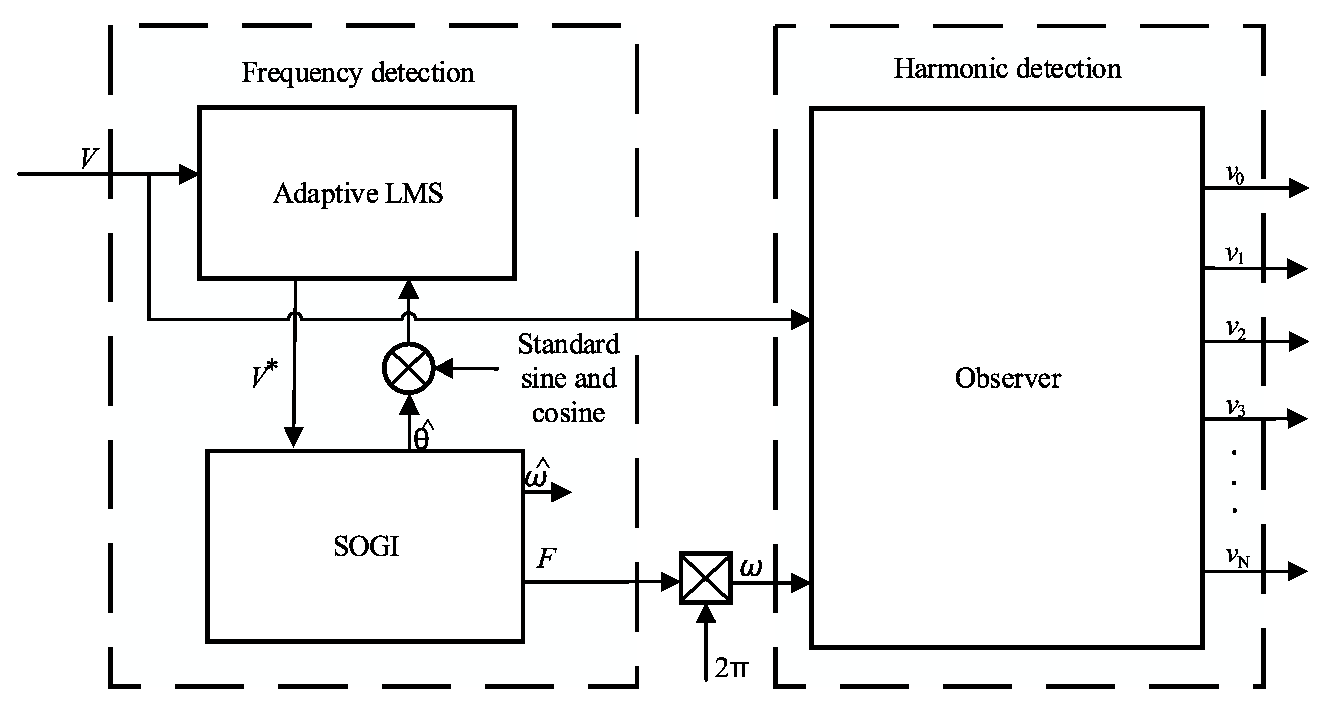
Figure 1 shows the detection principle of the proposed method.
The paper is structured as follows:
Section 2 conducts a theoretical analysis of the designed frequency detection algorithm and Luenberger observer;
Section 3 conducts a simulation verification;
Section 4 sets three different situations for the proposed harmonic extraction method to verify its accuracy and robustness;
Section 5 compare and discuss the proposed method with other methods;
Section 6 provides the conclusions.
2. Methods
Considering that the power grid is not in an ideal state during operation, the frequency and amplitude of power grid voltage may fluctuate due to the interference of various factors. Therefore, before using the observer to detect the harmonics of the input signal, it is necessary to obtain the real-time frequency information of the input signal. In the first part of this section, to obtain the real-time frequency of the input signal, the cascaded SOGI algorithm, which can avoid the influence of DC component, is designed. The second part uses the obtained real-time frequency to construct a time-varying composite observer; the harmonic components of each order contained in the signal are extracted in real time.
2.1. Fundamental Frequency Detection
SOGI can realize real-time phase detection in the changing power grid environment, while avoiding the limitations of traditional phase-locked loops and frequency-locked loops in the unbalanced power grid. When the grid is unbalanced, it can also detect the positive and negative power of the grid voltage. In addition, it has a high phase-locking accuracy and fast convergence speed. The advantages of the SOGI algorithm will be explained in further detail below. The phase detection principle of SOGI is shown in
Figure 2.
Where
represents the frequency at which the SOGI allows the signal to pass, and is also the resonant frequency of the resonant link in the figure. The transfer function expression of the resonance link in the figure is as follows:
Combined with the principle block diagram, the closed-loop transfer functions of the two systems can be obtained as follows:
where
is the transfer function of the band-pass filter,
is the transfer function of the low-pass filter, and
k affects the bandwidth of the closed-loop system.
When the grid voltage signals contain DC component, the traditional SOGI method will be affected by the DC component, so it can not accurately extract the positive sequence component of the signal. To eliminate the influence of the DC component, a cascade single-phase adaptive frequency locking method is proposed in this paper. Before the frequency of the input voltage signal is extracted by the SOGI algorithm, an adaptive LMS algorithm is cascaded to filter the DC components contained in the input signal.
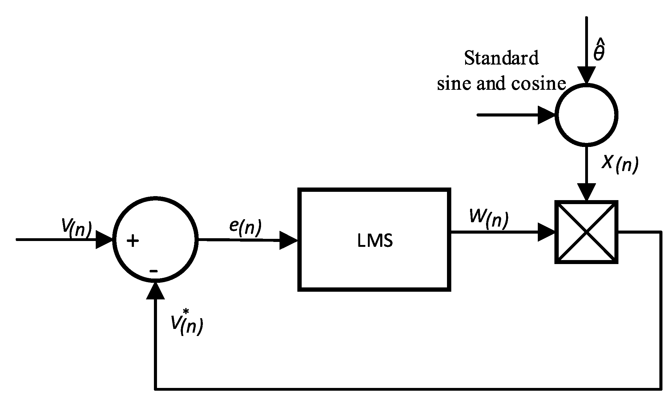
Figure 3 shows the principle of the cascaded adaptive LMS algorithm.
Where
,
,
represents the input grid voltage signal containing DC bias information,
represents the output signal after the DC component is filtered by the LMS,
is the system state error, and
represents the weight coefficient,
and
, respectively, represent a standard cosine signal and a sine signal with the phase
obtained by SOGI as a reference. The algorithm can be expressed as:
where
represents the iterative step size of the algorithm. The value will affect the convergence speed and stability of the algorithm. In this paper,
= 0.05.
The LMS algorithm filters the DC component of the input signal according to the given standard cosine signal and sine signal. Then the output signal is compared with the input signal , the system state error is caluclated, and the weighting coefficient of the LMS algorithm is updated. When the system is running, is constantly updated, so that the system state error tends towards zero, and the filtered signal can remove the DC component. The improved SOGI algorithm avoids the influence of DC component and accurately extracts the frequency of the input signal.
2.2. Observer Design
In general, an ideal single-phase power grid signal can be described as:
where
A represents the amplitude of the signal,
represents the angular frequency,
f is the fundamental frequency of the grid voltage, and
is the initial phase.
In the real operating environment, due to the existence of various disturbances, the grid voltage will be distorted. For a distorted signal,
can be modeled as the sum of a dc component and fundamental wave and various harmonic components.
can be set to:
Regarding each component of the input signal as a single sub-block,
, there are
modules in total, and the input signal is reset to:
To construct a dynamic system, a virtual quadrature component is introduced to the parameters in each module. For each individua module:
The dynamic system structure is described as:
where:
The observability criterion can be used to prove that the designed observer is observable. Formula (
12) shows that the observability matrix
O is full rank. The system simulated by the observer is stable, and its closed-loop poles can be arbitrarily configured.
A time-varying Luenberger observer was designed. The same model was constructed, based on the power system of Formulas (
9) and (
10). The difference was that the output error
of the observer was introduced and used to modify the estimation model of the system, so that the observed value
of the observer approaches the actual state
x of the system.
where:
L is the gain matrix of the observer error.
The error between the state
x of the system was defined, and its estimated value was
as
. The following dynamic system was constructed with respect to error
x.
The roots of the differential equation error can be located on the left-hand side (LHS) of the s-plane by the “pole placement” method. The configured root is also defined as the observation pole. By adjusting the position of the observation pole, the error between the observation value and the actual signal is close to 0, and an accurate estimation of the input signal is realized.
Figure 4 shows the principle of the observer designed in this paper.
Formula (13) can be described as:
Define the sampling period as Ts, at the (
k) moment, the continuous observer is written in a discrete form, and the estimated value of each state at the (
) moment is as follows:
3. Simulations
Usually, grid signals are distorted due to the presence of various disturbances. The harmonic components of the distorted grid signal are mainly concentrated on the 5th and 7th harmonic components [
26]. At the same time, the frequency and amplitude of the fundamental wave of the signal are often changed in the distorted power grid signal. When the observer performs harmonic extraction, the fundamental frequency information of the input signal first needs to be obtained. Therefore, the accuracy of the frequency estimation result directly affects the harmonic extraction result.
According to Formulas (
6) and (
7), the expression of the input signal is as follows:
Figure 5a simulates the frequency fluctuations in the fundamental frequency of the distorted grid signal. Usually, the grid frequency fluctuates between 48 Hz and 52 Hz, and the fluctuation range selected in this paper is the jump in the original signal from 49 Hz to 51 Hz.
Figure 5b shows the frequency estimation result when the fundamental amplitude of the grid signal changes. The fundamental amplitude of the input signal jumps to 1.2 times the original signal at the jump point.
Figure 5c is the frequency estimation result when the initial phase angle is changed. To show the effect of changing the phase angle, the phase shift is set to
/8. The three subplots in
Figure 5 show the estimation results of traditional SOGI, Recursive Least Squares (RLS), Three-Consecutive-Sample (3CS), and the cascaded SOGI frequency detection method proposed in this paper in three different cases, where the DC component of the input signal is set to 2 and the transition point is set at 1.357 s. The parameters in the simulation model are shown in
Table 1.
It can be seen from the estimation results that the traditional SOGI method has good convergence speed and stability in the case of grid distortion; however, due to the influence of the DC component, there is a large deviation between the estimation result and the actual fundamental frequency. To ensure the performance of the SOGI algorithm, this paper adopts the method of cascaded LMS to avoid the influence of the DC component on SOGI. The results show that compared with the traditional SOGI, the cascaded SOGI can accurately extract the frequency information of the input signal under the premise of ensuring convergence speed and stability.
Three cases of the dynamic convergence process, RLS, 3CS, and cascaded SOGI, were compared. It can be seen that when the fundamental frequency of the input signal changes, the three methods have different degrees of jitter, but all can complete the convergence within 60 ms. Among them, the convergence speeds of 3CS and cascaded SOGI are almost the same, but the fluctuation in the former is relatively large. RLS has better stability than cascaded SOGI and 3CS, but the convergence speed is not as fast as the first two methods. The cascaded SOGI algorithm achieves a better balance between convergence speed and stability.
The harmonic extraction result of the adopted observer under the condition of
is shown in
Figure 6a. It can be seen from the result that the observer can track the input signal within 0.05 s (three sampling periods). The observation error curve is shown in
Figure 6b, which converges to the vicinity of zero after 0.05 s.
In the case that the input signal may have unknown order harmonics, it is necessary to verify whether the adopted method is effective. Keep the original input signal unchanged, and truncate the harmonic detection algorithm of the observer to the fundamental, fifth, and seventh harmonics.
Figure 7 shows the harmonic extraction effect of the harmonic algorithm after truncating a specific frequency.
The observer error curve shown in
Figure 7b has increased fluctuations compared with
Figure 6b, but it can still converge to be near 0 after 0.05 s.
The results show that by comparing the detection error with the harmonic detection under the given conditions, the detection error after intercepting a specific frequency is still small. Therefore, the harmonic detection algorithm used in this paper shows strong robustness.
Figure 8 shows the result of harmonic detection when the input signal contains white noise. Among them, SNR is set to 5. From the results shown in
Figure 8a, it is found that even if there is severe noise interference in the input signal, the observer can still accurately extract the harmonics. From the observation error curve in
Figure 8b, the maximum error does not exceed 5, and the steady-state error after convergence is stable at about 2 (fundamental amplitude is 100).
Figure 9 shows the detection results of each harmonic contained in the input signal, where the fundamental frequency is 49 Hz. It can be seen that the results of each order of harmonic extraction are almost the same as the settings.
To verify the accuracy of the proposed algorithm,
was taken to represent the standard deviation of the observation error relative to the fundamental amplitude (
), and the calculation formula is as follows.
represents the calculation of the standard deviation; the calculated results are shown in
Table 2.
4. Experiments
The previous section discussed the influence of the distorted grid signal on the frequency estimation. To verify the possible influence of these changes on harmonic extraction, three cases of distorted grid signal changes were tested on the Speedgoat experimental platform. Speedgoat is a real-time system developed by mathworks based on the Simulink Real-Time toolbox of MATLAB, which can truly realize a seamless connection with MATLAB/Simulink. It is mainly used in the Rapid Control Prototype (RCP) and Hardware-In-Loop (HIL), which saves a lot of time in algorithm and hardware verification. The Speedgoat hardware can be flexibly configured according to user needs, and the software part only needs to use MATLAB/Simulink and its related toolbox, without additional software. This article builds an RCP loop using the Speedgoat component.
The experimental platform is shown in
Figure 10, which is composed of a host computer, Speedgoat real-time target machine, and NI-CompactRIO-9049. At first, the Simulink model is compiled to the Speedgoat real-time target machine through the Ethernet connection, and the signal to be tested is sent out by NI 9263, and then input to the real-time target machine through the analog input port of IO 102 board. There, the sampling frequency of the analog voltage signal sent by NI 9263 is
kHz.
4.1. Frequency Fluctuation
When the input signal reaches the set jump point of 1.357 s in the running time, the fundamental frequency jumps from 49 Hz to 51 Hz of the original signal. While jumping, other input signal parameters remain unchanged, and the input signal after jumping is shown in Equation (
20).
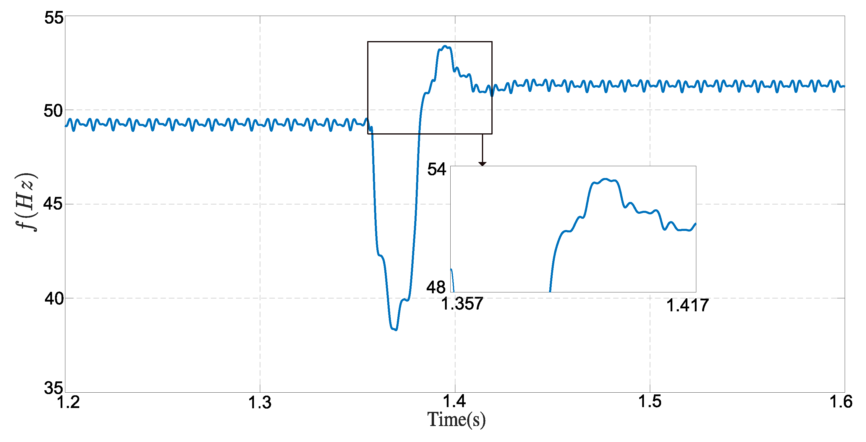
Figure 11 shows the dynamic convergence process of the frequency detection algorithm proposed in this paper when the fundamental frequency jumps. With the sudden change in the fundamental frequency of the input signal, the estimation result of the frequency detection algorithm shows a large drop at the jump point. This is because the new signal after the jump is equivalent to the translation of the original signal on the coordinate axis. As the algorithm parameters are updated, the frequency estimation result can re-track to the changed fundamental frequency. Moreover, the entire dynamic convergence process can be completed within 60 ms, and the estimated result after convergence is stable at around 51 Hz. This means that the frequency detection algorithm used in this paper can overcome the influence of fundamental frequency fluctuation and accurately re-estimate the frequency on the premise of ensuring fast convergence. It is worth noting that the traditional amplitude and phase detection time generally exceed 80 ms [
27].
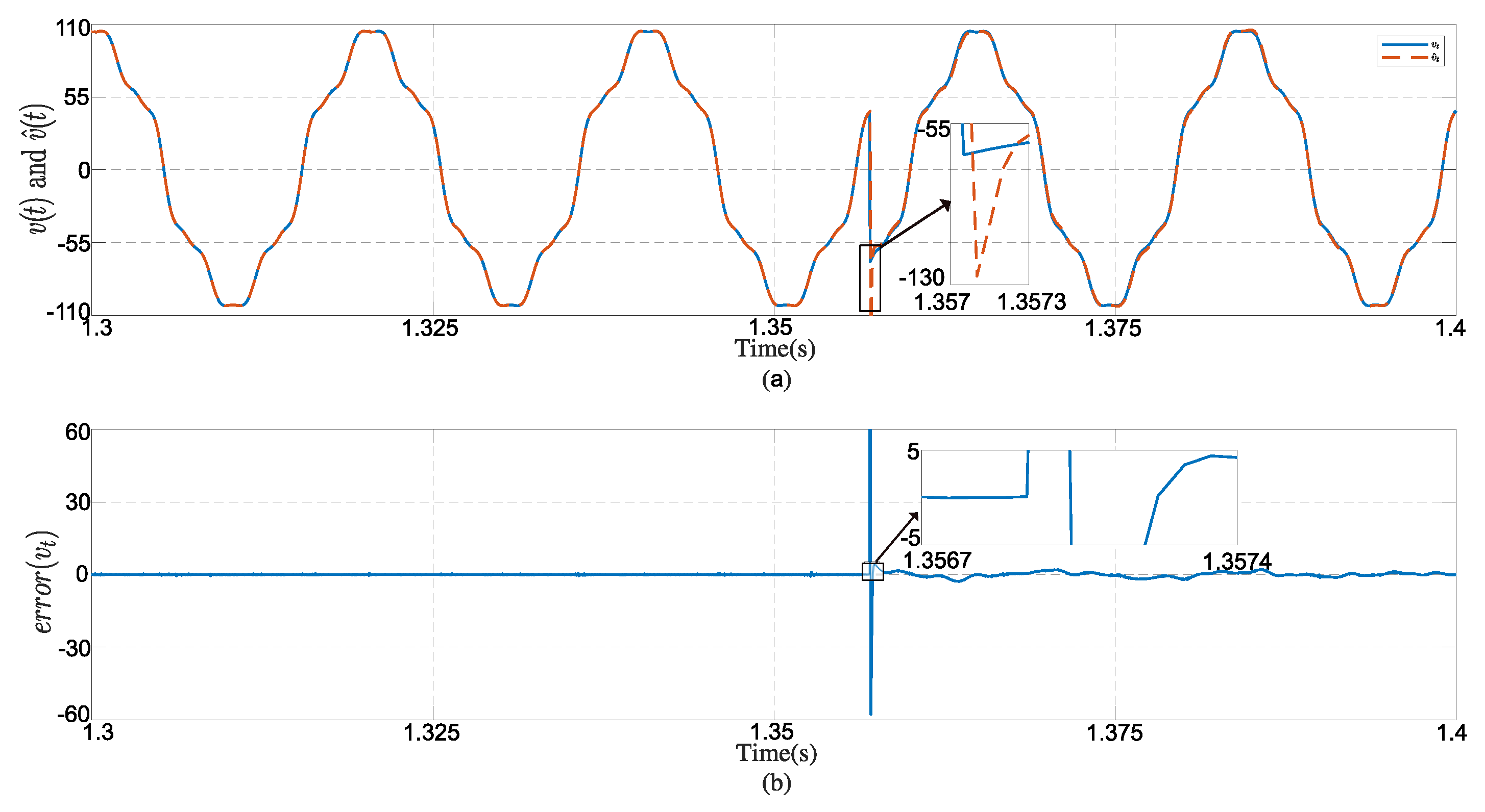
The harmonic detection results of the observer are shown in
Figure 12. Among them,
Figure 12a shows a comparison between the observer estimation result and the input signal when the fundamental frequency jumps. At the transition time of 1.357 s, the estimated value shows a large deviation compared with the input signal. This phenomenon is caused by the fact that the estimated value of the current observer is calculated based on the fundamental frequency of the previous cycle. As the fundamental frequency is updated, the observer’s estimate also retracks to the input signal. The specific convergence process is shown in
Figure 12b in the error curve between the observer estimate and the input signal. When the jump occurs, the error peak between the two signals is very large, but with an update to the algorithm, the error curve quickly returns to around 0 and converges within 60 ms. This means that the algorithm can re-estimate the input signal accurately within three cycles when the fundamental frequency fluctuates. It can be seen from
Figure 12 that during the whole harmonic detection process, the error curve of the observer can remain at a position near 0 after stabilization. Even if the input signal fluctuates, it can quickly converge. After stabilization, it is almost 0.
4.2. Amplitude Fluctuation
Fundamental wave amplitude fluctuation is also a frequent occurrence in distorted power grid signals. To verify the effectiveness of the proposed method when the fundamental wave amplitude changes, the fundamental amplitude of the input signal is set to jump at 1.357 s. The changed fundamental amplitude is 1.2 times that of the original input signal, and the other signal parameters remain unchanged. The input signal after the jump is shown in Equation (
21).
The frequency detection results before and after the fundamental amplitude jump are shown in
Figure 13. Compared with
Figure 11, it is found that the change in the frequency estimation result when the amplitude of the fundamental wave changes is obviously smaller, and is stable at around 49 Hz, and the fluctuation range does not exceed 1. At the same time, the convergence speed is consistent with the fundamental frequency change, and the convergence can also be completed within 60 ms. This may mean that changes in fundamental amplitude have less effect on the frequency estimation algorithm than changes in fundamental frequency, a phenomenon further illustrated by the observations shown in
Figure 14.
Figure 14a shows a comparison between the observer’s estimation result and the input signal when the amplitude of the fundamental wave changes. It can be seen that the deviation between the two signals after the transition is not as large as that when the frequency of the fundamental wave changes. As the frequency estimation are updated, the observer estimation can accurately track the input signal. The specific convergence process is shown in the observer error curve in
Figure 14b. Compared with the fundamental frequency change, the error curve of the observer, the error peak value at the transition has been significantly reduced, but the convergence speed of the two cases is similar, and the convergence can be completed within 60 ms. This shows that the accuracy of the harmonic detection method is greatly affected by the frequency estimation, and the greater the frequency fluctuation in the input signal, the greater the error between the observation result and the input signal. When the fundamental frequency converges to the real input signal frequency, the observer can complete the convergence within three cycles, and the error after stabilization is around 0.
4.3. Signal Phase Changes
To further verify the influence on the harmonic detection algorithm proposed in this paper when the input signal changes, a test is designed when the initial phase angle changes. As in the previous two experiments, only the initial phase angle was changed in the input signal, and to show the effect of changing the phase angle, the phase shift was set to at 1.357 s.
The frequency detection results in
Figure 15 show the whole convergence process of the estimated fundamental frequency when the initial phase angle of the input signal abruptly changes. Similar to the results of the previous two tests, the sudden change in the signal’s initial phase angle causes the frequency estimation result to become distorted again; however, because the fundamental frequency of the input signal after the jump remains unchanged, the frequency estimation result converges to the initial value of 49 Hz within 60 ms. The dynamic convergence process when the initial phase angle changes is similar to that when the fundamental frequency changes. In contrast, when the amplitude changes, it has the lowest influence on the estimation of fundamental frequency. The results of three tests show that the frequency detection algorithm quickly converges in the case of a fundamental frequency jump, amplitude jump and phase angle shift, and it shows good robustness.
The two sub-images in
Figure 16 show a comparison between the observer observation results and the input signal when the initial phase angle suddenly changes. Similar to the first two test results, the observation results deviate after the sudden change in phase angle. The reason for the deviation is similar to the fundamental frequency jump, because the new signal is equivalent to the displacement of the original signal on the coordinate axis. With the update of real-time frequency, the observation results are tracked to the input signal again. The error curve is shown in
Figure 16b; the peak value of the error curve after an abrupt change is the same as that of the abrupt change in fundamental frequency abrupt, and the peak value of the error curve when the amplitude changes is the smallest. However, the results of the three tests can converge again when the input signal changes, and the convergence rate is kept within 60 ms, about three cycles.
In sum, it can be concluded that the change in the input signal will directly affect the result of the frequency estimation, and the harmonic detection of the observer will also be biased with the distortion of the frequency estimation. However, as the frequency estimates converge, the observations eventually retrack to the input signal. Through the tests of three simulated distorted power grid signals, this paper proves that the method can resist fundamental frequency fluctuation, amplitude jump and phase angle change, and can re-estimate the input signal within 0.06 s after fluctuation. The dynamic convergence process of the error curve between the estimation result and the input signal proves the stability and accuracy of the method.
5. Discussion
For the effectiveness of the harmonic detection algorithm proposed in this paper, three cases of simulated distorted grid signals are discussed. It is undeniable that the disturbance phenomena that may occur in the actual operation of the power grid are more than these, but these three situations are representative of the distorted signal.
FFT is a practical harmonic analysis tool. Although it can only extract harmonics through offline analysis, the accuracy of harmonic extraction is very high and will not be attenuated as the order increases. Ref. [
18] proposed an input observer theory based on the observer method. The method constructs a state space equation by integrating the input signal, and can accurately extract the desired harmonic components in the case of grid current imbalance and fundamental frequency disturbance harmonics. For the three cases shown in
Section 4, the harmonic extraction method proposed in this paper is used for comparisons between FFT and input observer. Since the focus on the test is to compare the performance of the harmonic extraction, therefore, the fundamental frequency and phase information required by the two methods are obtained by cascading SOGI. The simulation is carried out on the MATLAB/Simulink toolbox platform and tested on the Speedgoat RCP platform.
When the signal fluctuates, the harmonic estimation results of the two methods will deviate from the input signal in different degrees.
Figure 17a,c,d shows the dynamic convergence process of the input observer and the proposed method in distorted power grid. As the input signal reaches a new stability after the transition, both methods can re-estimate the changed signal and complete the convergence. The difference is the time it takes to achieve convergence.
Figure 17b,d,f is the error curves between the harmonic estimation results of the two methods and the input signal when the fundamental frequency fluctuates, the amplitude jumps and the phase angle shifts, respectively. It can be seen from the figure that when the 1.357 s signal fluctuates, the two methods shake from the original stable state to different degrees, and then re-converge to around 0 in a certain period of time. The convergence process can be completed within 60 ms, reaching a new stable state. The difference is that the convergence time of the input observer is about 10 ms, 10 ms, and 20 ms longer than the proposed method, respectively, under the three signal fluctuation conditions set.
Table 3 compares the extraction results of the proposed method, FFT, and input observer for each order of harmonics contained in the input signal in steady state. Among them, the FFT analysis results are given by the FFT analysis module in MATLAB/Simulink. It can be seen from the table that the difference between the results of the three methods and the set value is not obvious, which proves that they all have accurate harmonic detection ability. However, the advantage of FFT is that the harmonic extraction accuracy of each order will not be attenuated with the increase of the harmonic order, which is incomparable with the other two methods.
Figure 18 is an experimental verification of the simulation results of
Figure 17, and the results also show the difference in the convergence speed of the two methods. Furthermore, it can be seen from the error curve after stabilization that the error of the input observer is larger than that of the proposed method.
Table 4 gives the standard deviation of the error curve after the transition has stabilized. It can be seen that the standard deviation of the error curve of the proposed method is less than 0.01% when it reaches the steady state again after completing the convergence, The standard deviation of the input observers is more than 1%.
It is worth noting that the method proposed in this paper has the advantages of not being limited by the hardware circuit topology, simple logic, and small amount of calculation.
Table 5 presents the computational load
occupied by the two methods during the test.
represents the task processing time, it can be seen in the Speedgoat control page, calculated as follows:
where,
represents the set step size, which is 0.00005.
According to
Table 5, it can be seen that the maximum computational load, minimum computational load, and average computational load required by the proposed method are, respectively, 1.04%, 1.36%, and 1.19% different from those of the input observer. Although the gap is not very obvious, in comparison, the method proposed in this paper can still achieve the purpose of saving computing resources.


