A Transferable Thruster Fault Diagnosis Approach for Autonomous Underwater Vehicle under Different Working Conditions with Insufficient Labeled Training Data

Abstract

Existing thruster fault diagnosis methods for AUV (autonomous underwater vehicle) usually need sufficient labeled training data. However, it is unrealistic to get sufficient labeled training data for each working condition in practice. Based on this challenge, a transferable thruster fault diagnosis approach is proposed. In the approach, an IPSE (instantaneous power spectrum entropy) and a STNED (signal-to-noise energy difference) are added to SPWVD (smoothed pseudo Wigner-Ville distribution) to identify time and frequency boundaries of the local region in the time-frequency power spectrum caused by thruster fault, forming a TFE (time-frequency energy) method for feature extraction. In addition, the RCQFFV (relative change quantity of the fault feature value), an MSN (multiple scale normalization) and a LSP (least square prediction) are added to SVDD (support vector data description) to align distributions of fault samples, contributing a TSVDD (transferable SVDD) for classification of fault samples. The experimental results of a prototype AUV indicate that the fault feature is monotonic to the percentage of thrust loss for the proposed TFE but not for the SPWVD. The TSVDD has a higher overall classification accuracy in comparison to conventional SVDD under working conditions with no labeled training data.

1. Introduction

Autonomous underwater vehicles (AUVs) are usually used to perform complex missions, such as ocean exploration, submarine observation, mapping, inspection of marine pipelines and structures, and so on [1,2]. Due to the difficulty in observing the working state of AUVs in the underwater environment, AUVs need enough autonomy to complete missions [3,4]. The autonomy is influenced by the propulsion system performances. Thrusters are commonly used components to constitute the propulsion system [5,6]. They bear strong working intensity. It makes them liable to become sources of faults [7,8]. Thruster faults result in thrust loss which means that the actual thrust of the thruster is less than the desired thrust under the same control command [9,10]. It may influence the completion of the missions and even threaten the security of AUVs [11,12].

The percentage of thrust loss is often used to describe the severity of thrust loss. For example, the percentage of thrust loss being λ% means that the ratio of the actual thrust to the desired thrust is (100 − λ)% [13]. It is important information for active fault-tolerant control to reconstruct a control law to keep the control of the AUV and even recover it [14,15]. Fault diagnosis is an effective way to identify the percentage of thrust loss for AUV thrusters [16]. Thruster fault diagnosis procedures generally begin with feature extraction, and then fault features extracted constitute fault samples. Finally, fault samples corresponding to different percentages of thrust loss are classified [17,18].

Among feature extraction approaches, data driven-based techniques which don’t require accurate AUV dynamic models are increasingly prevalent [19]. Wang et al. extract the amplitude feature of the wavelet detail coefficient in the frequency domain by wavelet transform [20]. The fault feature extracted is effective in fault detection. However, it is generally non-monotonic to the percentage of thrust loss. It means that the fault feature does not increase with the increase of the percentage of thrust loss, namely that the fault feature corresponding to a lower percentage of thrust loss may be bigger than the fault feature corresponding to a higher percentage of thrust loss. It leads to an overlapping distribution of fault samples corresponding to different percentages of thrust loss, which counts against fault sample classification. Sun et al. acquire the amplitude features of the singular signals in the time domain by modifying Bayes’ classification algorithm. The fault feature extracted is monotonic to the percentage of thrust loss. However, the extracted feature has strong volatility [21]. Considering the advantages and limitations of the above fault features extracted in the time domain or frequency domain, this article researches extracting fault features in the time-frequency domain. Among time-frequency analysis approaches, smoothed pseudo Wigner-Ville distribution (SPWVD) is a typical one. It is very suitable for obtaining the time-frequency power spectrum due to its quadratic time-frequency representation because the energy itself is a quadratic representation [22]. However, neither the maximum value of the time-frequency power spectrum nor the sum of the entire time-frequency power spectrum is monotonic to the percentage of thrust loss for AUV dynamic signals.

By further analysis of the time-frequency power spectrum of AUV dynamic signals, it is found that the signal energy generated by thruster faults mainly concentrates in a local region. Based on these findings, a novel time-frequency energy (TFE) method is proposed to extract the fault feature in this article. The basic idea of the TFE is to get the energy in the local region as a thruster fault feature. To achieve this, The TFE adds three contents to SPWVD. Firstly, an instantaneous power spectrum entropy (IPSE) is proposed to recognize the time boundaries of the local region. Secondly, a signal-to-noise energy difference (STNED) is developed to identify the frequency boundaries. Thirdly, the sum of the energy within the time and frequency boundaries is identified as a fault feature. Experimental results indicate that the fault feature extracted by the TFE is monotonic to the percentage of thrust loss.

Feature extraction is followed by fault sample construction and classification. Among fault sample classification methods, classification model-based methods are widely researched. In these methods, continuously varying percentage of thrust loss is divided into discrete severity levels of thrust loss. For example, at severity level one, the percentage of thrust loss is λ₁%. The fault sample obtained at severity level one is given label one. In the same way, at severity level two, the percentage of thrust loss is λ₂%. The fault sample obtained at severity level two is given label two, and so on. The fault samples with labels are called labeled samples. The labeled samples used to train a classification model are called labeled training data. Classification model-based methods first establish a classification model structure based on some algorithms, and then train the model parameters using labeled training data. Finally, fault samples with unknown labels are classified by the model, and their labels are estimated. According to the estimated labels, the percentages of thrust loss corresponding to the fault samples are obtained. For instance, if the estimated label is one, then the percentage of thrust loss is λ₁%.

Abed et al. constructed a classification model based on the dynamic recurrent neural network [23]. It has good fault sample classification performance under two rotational speed conditions of the thruster. Jiang et al. establish fault sample classification models based on the combination of a wide convolutional neural network and extreme learning machine under eight rotational speed conditions of thruster [24]. The authors construct separate fault sample classification models based on support vector data description (SVDD) under two surge speed conditions of the AUV. Different speed conditions mean different working conditions for the thruster in this article. In these methods, there is sufficient labeled training data under each working condition. Due to that the working condition of the autonomous underwater vehicle may change continuously in practice, there will be an infinite number of working conditions. It is unrealistic to get sufficient labeled training data for all working conditions. To solve this problem, using the classification model established under the working conditions with sufficient labeled training data to classify fault samples under another working condition with no labeled training data is a practical and feasible way. However, when the authors continue to use SVDD to do this, it is found that the overall classification accuracy is low.

After further analysis of the distribution of fault samples, it is found that the distribution of fault samples is very different under different working conditions. According to this, a new transferable SVDD (TSVDD) method is proposed to classify fault samples in this article. The basic idea of the TSVDD is to align the distribution of fault samples under different working conditions before training and testing the classification model. To achieve this, the TSVDD adds three pretreatments to SVDD. Firstly, the relative change quantity of the fault feature value (RCQFFV) is applied to reduce the range discrepancy of fault features extracted from different kinds of signals. Secondly, a multiple-scale normalization (MSN) is proposed to reduce the distribution differences of the same fault features obtained under different working conditions. Thirdly, a least square prediction (LSP) is proposed to estimate the unknown normalization scale under the working condition with no labeled training data. Experimental results show that the TSVDD has better overall classification accuracy in comparison to SVDD under the working condition with no labeled training data.

Above all, the main contribution of this article is that a novel transferable thruster fault diagnosis approach consisting of TFE and TSVDD is presented for AUVs. The TFE is developed from SPWVD to make the fault feature monotonic to the percentage of thrust loss. The TSVDD is improved from SVDD to increase the overall identification accuracy.

The rest of this article is organized as follows. The TFE and TSVDD are described in detail in Section 2 and Section 3, respectively. Experimental validations are shown in Section 4. Conclusions are drawn in Section 5.

2. TFE Approach

2.1. Conventional SPWVD

SPWVD is a suitable technique to derive the power spectrum due to its quadratic representation. The formula of SPWVD can be expressed by Equation (1) [25].

$$\mathrm{SPWVD}\left(n,m\right)=2\left|{\displaystyle \sum _{k=-\left(L-1\right)}^{L-1}h\left(k\right)}{\displaystyle \sum _{l=-\left(M-1\right)}^{M-1}g\left(l\right)}z\left(n+l+k\right)z*\left(n+l-k\right)e^{\frac{-j2\pi km}{N_3}}\right|$$

(1)

where SPWVD(n,m) is the time-frequency power spectrum of AUV dynamic signals, h(k) and g(l) are smoothing window functions in the frequency direction and time direction, respectively, z(n) is the analytical signal of AUV dynamic signals, z*(n) is the complex conjugate of z(n), N₃ is the number of frequency bins, $\left|·\right|$ is the absolute value function.

After obtaining the time-frequency power spectrum, one way is to take the maximum value of the time-frequency power spectrum as the fault feature. However, in the experiment, it is found that the fault feature corresponding to a smaller percentage of thrust loss may be larger than that of a bigger percentage of thrust loss, making the fault feature non-monotonic to the percentage of thrust loss. Another way is to take the sum of the entire time-frequency power spectrum as a fault feature. Since the energy produced by a thruster fault mainly concentrates in a local region of the time-frequency power spectrum, when the sum of the whole time-frequency power spectrum is used as a fault feature, the energy outside the local region which is not caused by the thruster fault will also be included in the fault feature, resulting that the extracted fault feature is greater than the actual one. It leads that the fault feature is still not monotonic to the percentage of thrust loss. The third way sets a threshold first, and then all the time-frequency power spectrum larger than the threshold is added together to form a fault feature. Due to that the value corresponding to noise in the time-frequency power spectrum is larger than that corresponding to thruster fault in some cases, it is difficult to find an appropriate threshold.

2.2. Proposed TFE Approach

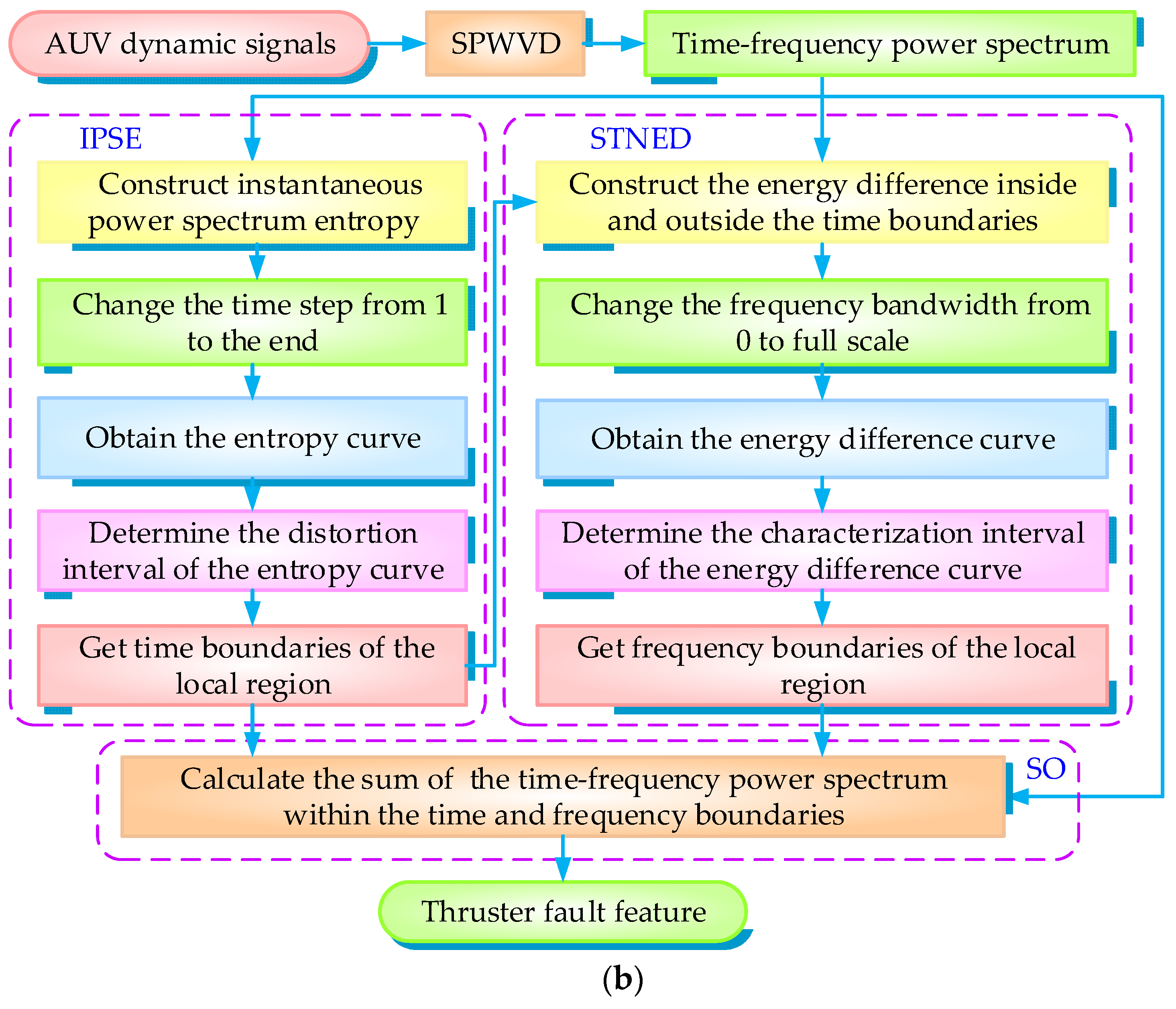
To find a way to get a fault feature monotonic to the percentage of thrust loss from the time-frequency power spectrum. The time-frequency power spectrums of the experimental data corresponding to different percentages of thrust loss are further analyzed. It is found that the time-frequency power spectrum of the AUV surge speed signal is uniform when the thruster works normally. The thruster fault causes the energy to migrate to a local region in the time-frequency power spectrum, forming an energy concentration. Moreover, the greater the percentage of thrust loss, the stronger the energy concentration. Inspired by the above results, a novel TFE method is proposed in this article. The basic idea of the TFE is to get the energy in the local region as a thruster fault feature. It recognizes the time and frequency boundaries of the local region in the time-frequency power spectrum, and then it regards the sum of the energy within the time and frequency boundaries as a fault feature. The flow chart of the proposed TFE method is illustrated in Figure 1.

As shown in Figure 1, the time-frequency power spectrums of AUV dynamic signals are obtained based on SPWVD. The thruster fault causes the energy to migrate to a local region. The IPSE is proposed to identify the time boundaries of the local region. The STNED is developed to get frequency boundaries of the local region. These are two new contents added by the TFE, while these don’t exist in conventional SPWVD. The TFE calculates the sum of the time-frequency power spectrum enclosed by the time and frequency boundaries, while conventional SPWVD adds up the entire time-frequency power spectrum or the time-frequency power spectrum larger than the threshold value.

The process of the proposed TFE is described in detail in the followings.

(1)

The IPSE-based time boundary identification

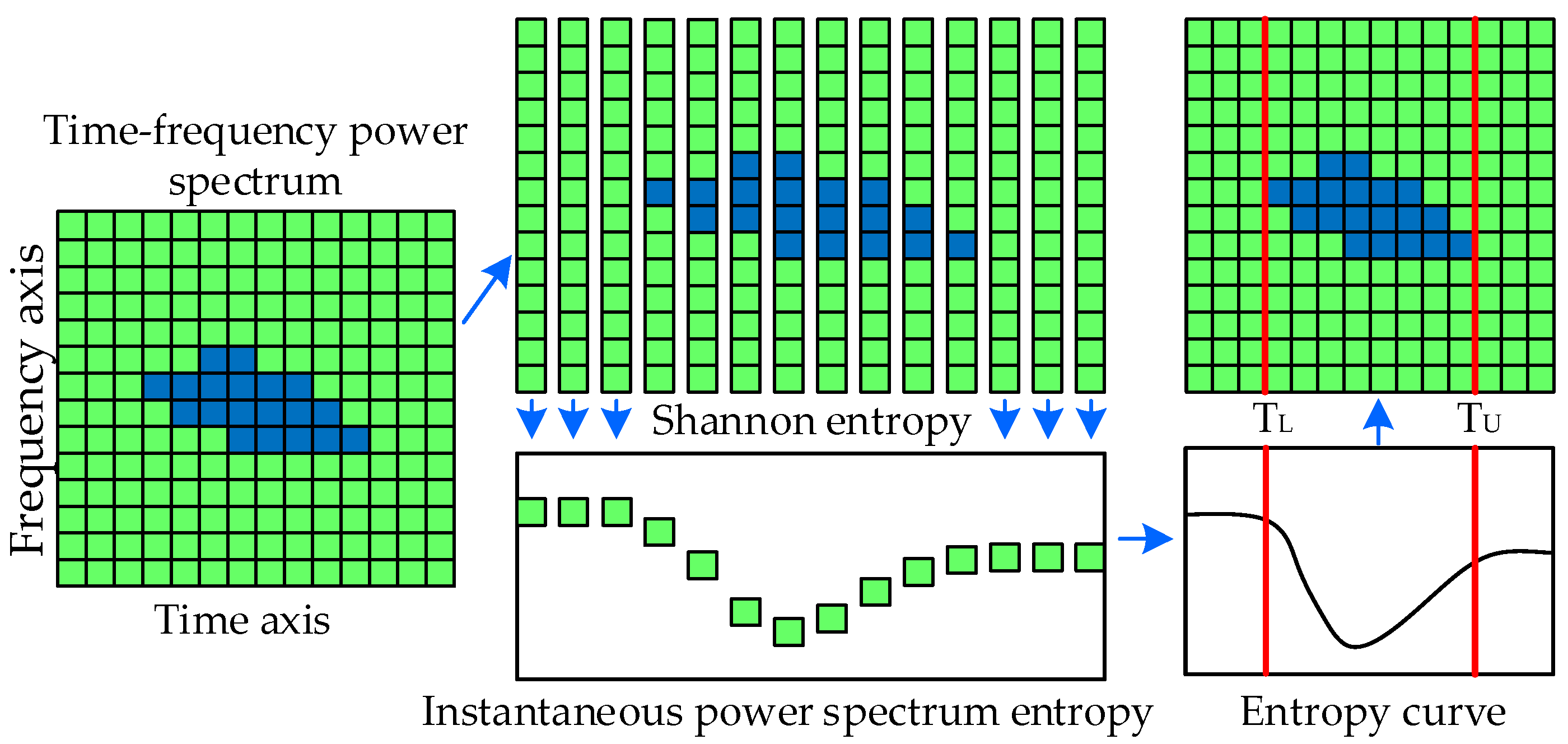
The schematic diagram of the proposed IPSE is shown in Figure 2. The basic idea of the IPSE is described as follows. Thruster fault produces a local concentration in the time-frequency power spectrum. The concentration promotes a signal energy migration from high frequencies to low frequencies. The energy distribution of the instantaneous power spectrum becomes uneven. The Shannon entropy of the instantaneous power spectrum decreases. It forms a distortion interval in the entropy curve, which is contributed by the Shannon entropy at each moment. The interval boundaries are regarded as time boundaries of the local region.

The instantaneous power spectrum entropy is calculated by Equations (2) and (3).

$$p\left(j,i\right)=\mathrm{SPWVD}\left(j,i\right)/{\displaystyle \sum _{i=1}^{N_1}\mathrm{SPWVD}\left(j,i\right)}$$

(2)

$$H\left(j\right)=-{\displaystyle \sum _{i=1}^{N_1}p\left(j,i\right)\lg p\left(j,i\right)}$$

(3)

where j is the time step, i is the serial number of frequency bins, $H\left(j\right)$ is instantaneous power spectrum entropy.

The distortion interval of the entropy curve is obtained by the following procedures. Find the location of the minimum entropy in the instantaneous power spectrum entropy curve. Go along the entropy curve from this location to the adjacent local maximum points on both sides. If the local maximum entropy is smaller than the minimum one in other regions, keep going until the local maximum entropy encountered is greater than the minimum value in other regions. The part between the final two maximum points contributes to the distortion interval of the entropy curve.

The left and right boundaries of the distortion interval are regarded as the lower-time boundary $T_U$ and upper-time boundary $T_L$ of the local region, respectively.

(2)

The STNED-based frequency boundary recognition

The schematic diagram of the proposed STNED is shown in Figure 3. The basic idea of the STNED is described as follows. The energy inside the time boundaries is generally smaller than the energy outside the time boundaries in the frequency bands with no fault information. Hereby, the greater the proportion of the fault information in a frequency band is, the bigger the energy difference inside and outside the time boundaries is. The frequency band corresponding to the maximum energy difference is recognized as the frequency boundary.

The energy difference inside and outside the time boundaries is calculated by Equation (4).

$$E_D\left(i\right)={\displaystyle \sum _{j=T_L}^{T_U}{\displaystyle \sum _{k=1}^i\mathrm{SPWVD}\left(j,k\right)}}-\left({\displaystyle \sum _{j=1}^{T_L}{\displaystyle \sum _{k=1}^i\mathrm{SPWVD}\left(j,k\right)}}+{\displaystyle \sum _{j=T_U}^{N_2}{\displaystyle \sum _{k=1}^i\mathrm{SPWVD}\left(j,k\right)}}\right)$$

(4)

where j is the time step, i and k are the serial number of frequency bins, $T_U$ and $T_L$ are the upper- and lower-time boundaries.

The frequency boundaries of the local region are determined by the following procedures. Find the location of the maximum value in the energy difference curve. This location is regarded as the upper frequency boundary $F_U$. Go along the energy difference curve from the upper frequency boundary to the left adjacent local minimum point. The location of the local minimum point is identified as the lower frequency boundary $F_L$.

(3)

The sum operation-based fault feature extraction

After recognizing the time and frequency boundaries of the local region, the sum of the energy in the boundaries is regarded as the fault feature. It is expressed in Equation (5).

$$F_{TFE}={\displaystyle \sum _{j=T_L}^{T_U}{\displaystyle \sum _{i=F_L}^{F_U}\mathrm{SPWVD}\left(j,i\right)}}$$

(5)

where $F_{TFE}$ is the fault feature, j is the time step, i is the serial number of frequency bins, $T_U$ and $T_L$ are upper and lower time boundaries, $F_U$ and $F_L$ are upper and lower frequency boundaries.

A novel fault feature extraction method, namely the TFE, is described in this section. The effectiveness of the TFE will be verified in Section 4.2.

3. The TSVDD Approach

3.1. Conventional SVDD

SVDD is an effective classification method. It constructs many separate one-class classifiers by treating each class of fault samples as target data, respectively. All one-class classifiers constitute a whole classifier. The minimum of the relative distances to each one-class classifier is used to decide which one-class classifier the test fault sample belongs to [26]. The detailed process is described as follows.

(1)

Construct one-class classifiers

The training samples $X_k=\left\{x_{ki}\right\}$ are brought into Equation (6) to seek a set of optimal solution ${\mathit{\alpha }}_k=\left\{{\alpha }_{ki}\right\}$ through a training process. In the optimal solution ${\mathit{\alpha }}_k=\left\{{\alpha }_{ki}\right\}$, most ${\alpha }_k{}_i$ are equal to zero, namely ${\alpha }_k{}_i=0$. A few ${\alpha }_{ki}$ are greater than zero, namely ${\alpha }_k{}_i>0$. The fault sample corresponding to ${\alpha }_k{}_i>0$ is called a support vector, given the symbol $x_{ksvi}$. Support vectors $x_k{}_{svi}$ are brought into Equation (7) to calculate the radius R_k of the one-class classifier.

$$\max L\left({\alpha }_k\right)={\displaystyle \sum _{i=1}^{N_4}{\alpha }_k{}_{i}K\left(x_{ki},x_{ki}\right)}-{\displaystyle \sum _{i=1,j=1}^{N_4}{\alpha }_k{}_i{\alpha }_{kj}K\left(x_{ki},x_{kj}\right)}$$

(6)

$$R_k^2=K\left(x_{ksvi},x_{ksvi}\right)-2{\displaystyle \sum _{i=1}^{N_4}{\alpha }_{ki}K\left(x_{ksvi},x_k{}_i\right)}+{\displaystyle \sum _{i=1,j=1}^{N_4}{\alpha }_{ki}{\alpha }_{kj}K\left(x_{ki},x_{kj}\right)}$$

(7)

where ${\displaystyle \sum _{i=1}^{N_4}{\alpha }_k{}_i}=1$, N₄ is the number of fault samples; $0\le {\alpha }_k{}_i\le C$, C is the penalty coefficient, $K\left(x_{ki},x_{kj}\right)=\exp \left(-{‖x_{ki}-x_{kj}‖}^2/{\sigma }_k^2\right)$, k is the severity level of thrust loss.

(2)

Establish the whole classifier

Repeat step (1) and obtain one-class classifiers corresponding to each severity level of thrust loss. All one-class classifiers are integrated to establish a whole classifier. The whole classifier is used for multi-class classification.

(3)

Testing samples classification

Bring a testing sample into Equation (8) to calculate the generalized distance from the testing sample to the center of the classifier.

$$D_k^2=K\left(x_U,x_U\right)-2{\displaystyle \sum _{i=1}^{N_4}{\alpha }_{ki}K\left(x_U,x_k{}_i\right)}+{\displaystyle \sum _{i=1,j=1}^{N_4}{\alpha }_{ki}{\alpha }_{kj}K\left(x_{ki},x_{kj}\right)}$$

(8)

where $D_k$ is the generalized distance, $K\left(x_{ki},x_{kj}\right)=\exp \left(-{‖x_{ki}-x_{kj}‖}^2/{\sigma }_k^2\right)$, $x_U$ is the testing sample.

Bring the generalized distance $D_k$ into Equation (9) to calculate the relative distance from the testing sample to the center of the classifier.

$${\epsilon }_k={D_k/R}_k$$

(9)

where ${\epsilon }_k$ is the relative distance, $D_k$ is the generalized distance, R_k is the radius of the classifier, k is the severity level of thrust loss.

The minimum relative distance ${\epsilon }_k$ is used to decide which one-class the testing sample belongs to.

When the whole classifier based on SVDD is applied to classify thruster fault samples, the results are described as follows. In the case that testing samples and training samples are drawn under the same working condition, the whole classifier has good classification performance. However, when the whole classifier established under one working condition with sufficient labeled training data is applied to classify testing samples under another working condition with no labeled training data, the classification accuracy decreases a lot.

3.2. Proposed TSVDD Method

To increase the classification accuracy in the case that the whole classifier established under one working condition with sufficient labeled training data is applied to classify testing samples under another working condition with no labeled training data, the distribution of original fault samples obtained under different working conditions is further analyzed. The results indicate that the range of one kind of fault feature is different from that of another kind of fault feature under the same working condition and that the distribution of one kind of fault feature obtained under one working condition is different from that of the same kind of fault feature obtained under another working condition.

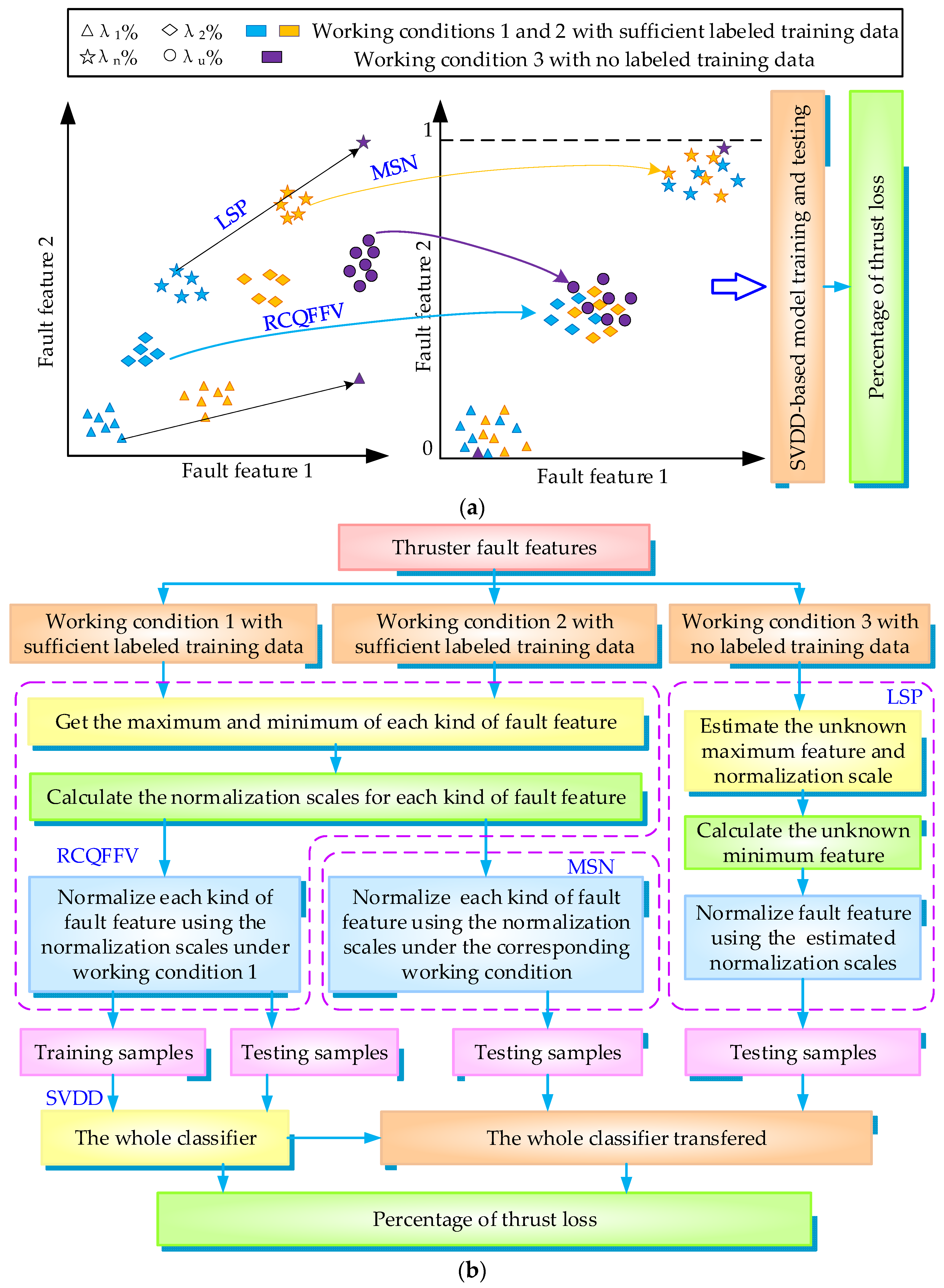
Motivated by the above results, a novel TSVDD is proposed in this article. The basic idea of the TSVDD is described as follows. It aligns the distributions of fault samples under different working conditions and uses the fault samples aligned to train and test the classification model. The flow chart of the proposed TSVDD method is illustrated in Figure 4.

As shown in Figure 4, the RCQFFV is applied to reduce the range discrepancy of fault features extracted from different kinds of signals under the same working condition. The MSN is proposed to reduce the distribution discrepancy of the same fault features obtained under different working conditions. The LSP is proposed to estimate the unknown normalization scale under the working condition with no labeled training data. These are three pretreatments added by the TSVDD, while these don’t exist in the conventional SVDD.

The process of the proposed TSVDD is described in detail as follows.

(1)

The RCQFFV-based range normalization of different kinds of fault features

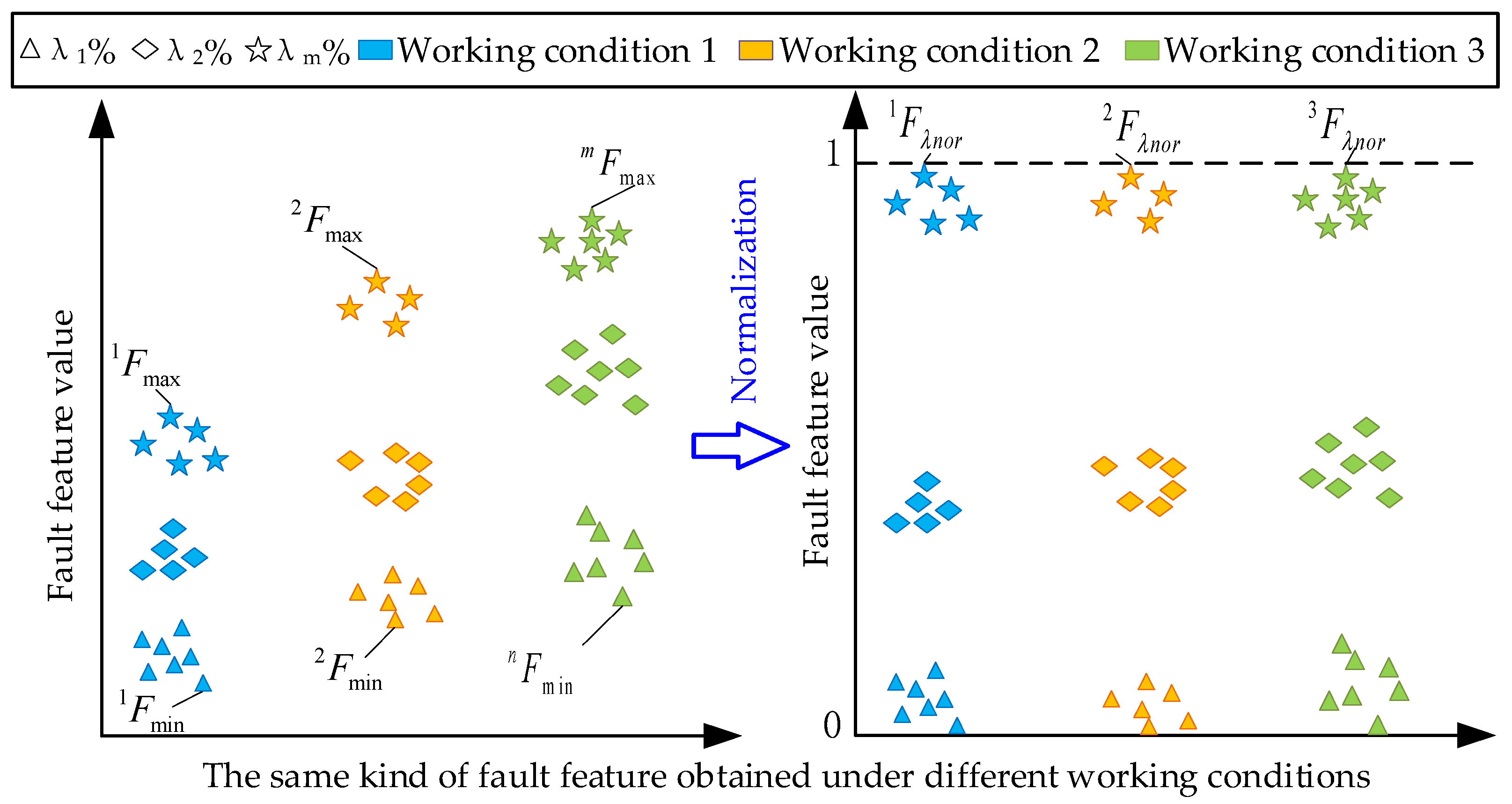
The schematic diagram of RCQFFV is shown in Figure 5. The basic idea of the RCQFFV is normalizing fault features to reduce the range discrepancy of fault features extracted from different kinds of signals.

The maximum and minimum values of each kind of fault feature are taken as their upper and lower limits, respectively. The difference between the maximum and minimum is taken as the normalization scale. The normalization process is expressed as Equation (10).

$${}_{n}F{}_{\lambda nor}=\frac{\left|{}_{n}F{}_{\lambda }-{}_{n}F{}_{\min }\right|}{\left|{}_{n}F{}_{\max }-{}_{n}F{}_{\min }\right|}$$

(10)

where ${}_{n}F{}_{\lambda nor}$ is the fault feature normalized, ${}_{n}F{}_{\lambda }$ is the fault feature corresponding to the percentage of thrust loss λ%, ${}_{n}F{}_{\min }$ is the minimum fault feature, ${}_{n}F{}_{\max }$ is the maximum fault feature, $\left|{}_{n}F{}_{\max }-{}_{n}F{}_{\min }\right|$ is the normalization scale. n is the code of a kind of fault feature.

Equation (10) indicates that the RCQFFV uses a single normalization scale to normalize the fault feature corresponding to different working conditions. When the single normalization scale matches the working condition, different kinds of fault features will have the same range after normalization. Otherwise, it does not. The same kind of fault features obtained under different working conditions still have a different range after normalization due to that one single normalization scale can only match one working condition.

(2)

The MSN-based range normalization under different working conditions

To reduce the distribution differences of the same fault features obtained under different working conditions, the MSN is proposed to normalize fault features. The schematic diagram of MSN is shown in Figure 6. The basic idea of the MSN is that it sets a separate normalization scale for each working condition.

The process of the MSN is expressed as Equation (11).

$${}^{m}F{}_{\lambda nor}=\frac{\left|{}^{m}F{}_{\lambda }-{}^{m}F{}_{\min }\right|}{\left|{}^{m}F{}_{\max }-{}^{m}F{}_{\min }\right|}$$

(11)

where ${}^{m}F{}_{\lambda nor}$ is the fault feature normalized, ${}^{m}F{}_{\lambda }$ is the fault feature corresponding to percentage of thrust loss λ%, ${}^{m}F{}_{\min }$ is the minimum fault feature, ${}^{m}F{}_{\max }$ is the maximum fault feature, m is the code of a working condition.

(3)

The LSP-based unknown normalization scale estimation

Since the working condition of AUVs may change continuously, there will be an infinite number of working conditions, making it unrealistic to get sufficient labeled training data to obtain separate normalization scales for all working conditions. When the fault feature under a working condition with no labeled training data is to be normalized, only the normalization scale under the working condition with labeled training data can be selected for the normalization process. However, in this situation, there is still a big distribution discrepancy of the same fault feature obtained under different working conditions.

To overcome this, the LSP is proposed. The schematic diagram of LSP is shown in Figure 7. The basic idea of the LSP is using the known normalization scales under working conditions with labeled training data to estimate the unknown normalization scale under the working condition with no labeled training data based on the least square algorithm.

The process of the LSP is described as follows.

Firstly, the unknown maximum fault feature is estimated by Equation (12).

$$\frac{\left|{}^{mu}F{}_{\max }-{}^{m1}F{}_{\max }\right|}{\left|{}^{mu}V-{}^{m1}V\right|}=\frac{\left|{}^{m2}F{}_{\max }-{}^{m1}F{}_{\max }\right|}{\left|{}^{m2}V-{}^{m2}V\right|}$$

(12)

where m₁, m₂, and m_u are the codes of working conditions, ${}^{m1}F{}_{\max }$, ${}^{m2}F{}_{\max }$, and ${}^{mu}F{}_{\max }$ are the maximum fault features under working conditions m₁, m₂, and m_u, respectively, ${}^{m1}F{}_{\max }$ and ${}^{m2}F{}_{\max }$ are known, ${}^{mu}F{}_{\max }$ is unknown and to be estimated, ${}^{m1}V$, ${}^{m2}V$, and ${}^{mu}V$ are the moving speeds of AUV corresponding to working conditions m₁, m₂, and m_u, respectively.

Secondly, the unknown normalization scale is estimated by Equation (13).

$$\frac{\left|{}^{mu}S-{}^{m1}S\right|}{\left|{}^{mn}V-{}^{m1}V\right|}=\frac{\left|{}^{m2}S-{}^{m1}S\right|}{\left|{}^{m2}V-{}^{m1}V\right|}$$

(13)

where ${}^{m1}S$, ${}^{m2}S$, and ${}^{mu}S$ are the normalization scales under working conditions m₁, m₂, and m_u, respectively, ${}^{m1}S$ and ${}^{m2}S$ are known, ${}^{mu}S$ is unknown and to be estimated.

Thirdly, the unknown minimum fault feature is calculated by Equation (14).

$${}^{mu}F{}_{\min }={}^{mu}F{}_{\max }-{}^{mu}S$$

(14)

where ${}^{mu}F{}_{\min }$ is the minimum fault feature estimated under working condition m_u.

Finally, ${}^{mu}F{}_{\max }$ and ${}^{mu}F{}_{\min }$ are brought into Equation (11) to normalize fault feature under working condition m_u.

(4)

The SVDD-based classification of fault samples

A whole classifier is established under the working condition with sufficient labeled training data based on SVDD using the fault feature normalized by the RCQFFV. The whole classifier is transferred to a new working condition. If the new working condition is the same as the original one, then the testing sample is normalized by the RCQFFV. If the new working condition is different from the original one, but it has sufficient training data, then the testing sample is normalized by the MSN. If the new working condition is different from the original one and it has no labeled training data, then the testing sample is normalized by the LSP. The testing sample normalized is brought into the whole classifier. The percentages of thrust loss corresponding to testing samples are obtained.

A novel fault sample classification method, namely the TSVDD, is described in this section. The effectiveness of the TSVDD method will be verified in Section 4.3.

4. Experimental Results and Discussion

4.1. Experimental Set up and Data

To verify the effectiveness of the proposed methods, namely the TFE and the TSVDD, pool experiments with an experimental prototype of AUV are conducted. The physical layout of the AUV is shown in Figure 8. It installed two horizontal surge thrusters, namely HT3 and HT4, and two horizontal auxiliary thrusters, namely HT1 and HT2. The surge speed of AUV is obtained based on HT3 and HT4. The heading angle is adjusted by HT1 and HT2.

The experimental process is described as follows. The target surge speed of the AUV is set at u_T m/s. AUV starts from 0 m/s. The fault of HT3 occurs at time step 250 and continues to the end of the experiment. The percentage of thrust loss is set at λ%. The thruster fault is simulated by decreasing the control voltage which is actually loaded to the thruster driver. The experimental data including the control voltage for main thrusters and the surge speed of AUV is recorded at 5 Hz. The target surge speed u_T is 0.2 m/s, 0.3 m/s, 0.4 m/s, and 0.5 m/s, respectively. The λ% is 0%, 10%, 20%, 30%, and 40%, respectively. The experimental data under a target surge speed of 0.3 m/s and with a percentage of thrust loss of 30% is taken as an example, as shown in Figure 9.

As shown in Figure 9, AUV starts up at time step 1, and it begins sailing at a steady speed of 0.3 m/s after time step 100. This article researches thruster fault diagnosis at stable speeds, so the data from time step 101 to time step 600 are selected. According to the selected data, the surge speed signals with different percentages of thrust loss are more clearly expressed in Figure 10a. In addition, the change rate of the control voltage is calculated. The results are displayed in Figure 10b.

4.2. Experimental Validation of the TFE Method

To validate the effectiveness of the TFE method, the TFE and many competitive methods are used to extract fault features. The experimental process and the results are presented as follows.

(1)

Experimental validation of the IPSE

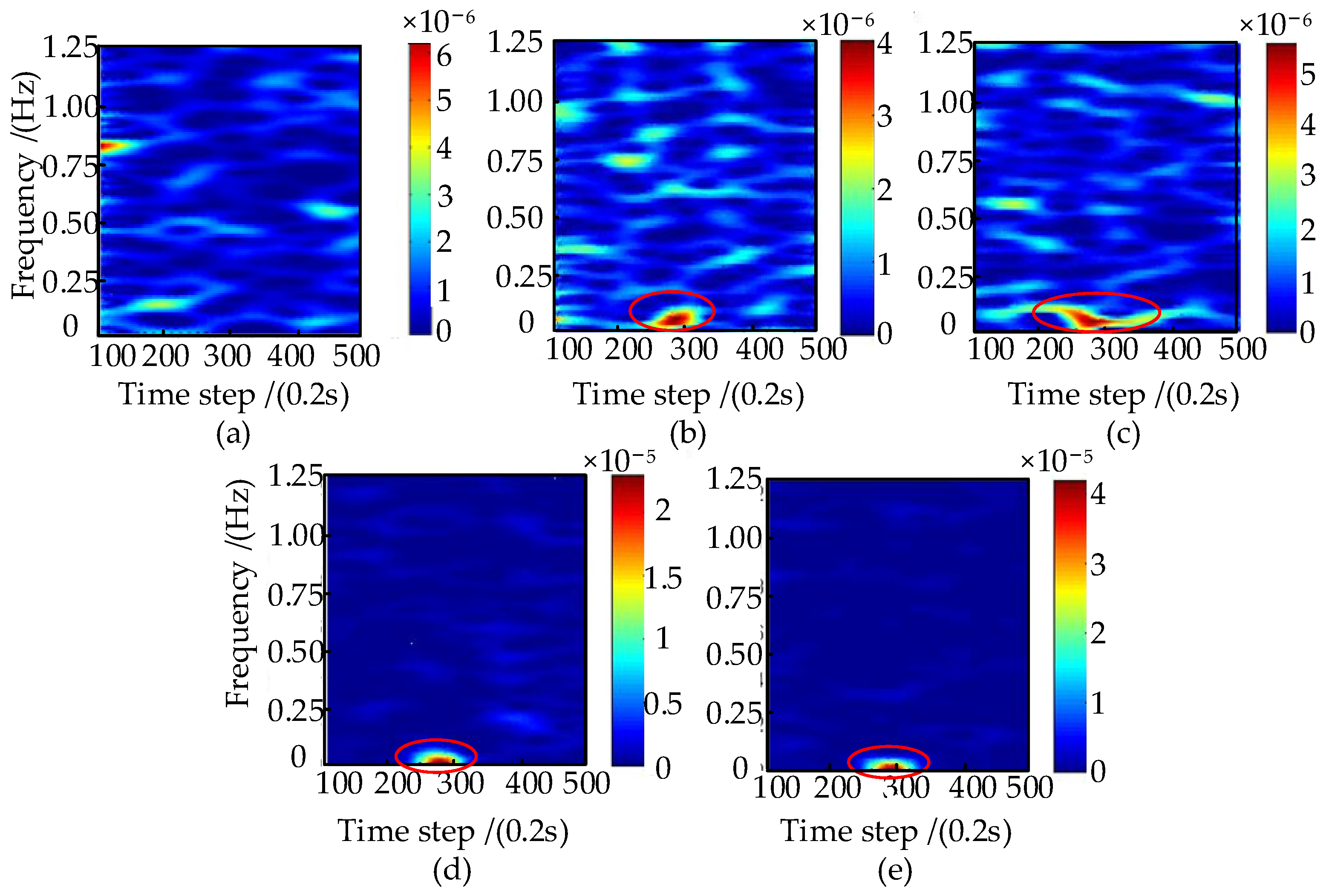
The AUV surge speed data corresponding to percentages of thrust loss 0%, 10%, 20%, 30%, and 40% shown in Figure 10 is selected as example data. The time-frequency power spectrums of the example data obtained based on SPWVD are displayed in Figure 11.

It is found that the time-frequency power spectrum of the AUV surge speed signal is uniform when the thruster works normally. The thruster fault causes the energy to migrate to a local region in the time-frequency power spectrum, forming an energy concentration as shown in the red circles. Moreover, the greater the percentage of thrust loss, the stronger the energy concentration.

To validate the effectiveness of the IPSE, the time-frequency power spectrums corresponding to percentages of thrust loss 10%, 20%, 30%, and 40% shown in Figure 11b–e are selected as example data. The IPSE is applied to analyze the example data. The instantaneous power spectrum entropy curves derived are shown in Figure 12.

As shown in Figure 12a, the minimum of the entropy curve corresponding to the percentage of thrust loss of 10% is 4.982 at time step 283. Its adjacent maximum on the left is 5.311 at time step 226, and the one on the right is 5.366 at time step 332. Therefore, the distortion interval of the entropy curve is [226 332]. The time boundaries of the local region are [226 332]. Similarly, the time boundaries are [174 314], [211 337], and [192 387], corresponding to percentages of thrust loss of 20%, 30%, and 40%, respectively. The time boundaries of the local region are set in Figure 13.

As shown in Figure 13a, the two white vertical lines are time boundaries, and the local concentration region marked with the red circle is caused by the thruster fault. It is found that the local region is closely surrounded by time boundaries. Similarly, the local regions corresponding to percentages of thrust loss of 20%, 30%, and 40% are also closely surrounded by the time boundaries as shown in Figure 13b–d. The results indicate that the proposed IPSE has a good performance in recognizing the time boundaries of the local region.

(2)

Experimental validation of the STNED

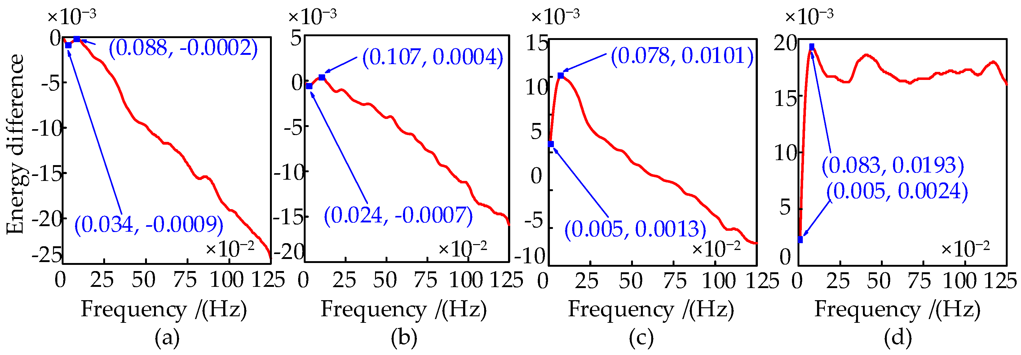
The STNED is used to analyze the example data displayed in Figure 13. The energy difference curves obtained are shown in Figure 14.

As shown in Figure 14a, the maximum of the energy difference curve corresponding to the percentage of thrust loss of 10% is −0.0002 at frequency 0.088. The left adjacent local minimum is −0.0009 at frequency 0.034. Therefore, the frequency boundaries of the local region are [0.034 0.088]. Similarly, the frequency boundaries are [0.024 0.107], [0.005 0.078], and [0.005 0.083] corresponding to the percentages of thrust loss of 20%, 30%, and 40%, respectively. The frequency boundaries of the local region are set in Figure 15.

As shown in Figure 15a, the white horizontal lines are frequency boundaries. It is obtained that the local region is enclosed by frequency boundaries. This phenomenon is also shown in Figure 15b–d. It indicates that the frequency boundaries delineated by the proposed STNED are consistent with the actual frequency boundaries of the local region.

(3)

Experimental validation of the TFE method

The methods proposed TFE, SPWVD+MV, SPWVD+SO, SPWVD+TH+SO, SPWVD+IPSE+SO, SPWVD+IPSE+SFPSE+SO, are used to extract fault features from the selected data shown in Figure 10a. For convenience, detailed descriptions of the methods are given in the followings. SPWVD+MV gets the time-frequency power spectrum of the signal based on SPWVD and takes the maximum value of the time-frequency power spectrum as a fault feature. SPWVD+SO takes the sum of the entire time-frequency power spectrum as a fault feature. SPWVD+TH+SO sets a threshold and adds all the time-frequency power spectrums larger than the threshold together to form a fault feature. SPWVD+IPSE+SO identifies the time boundaries of the local region based on IPSE and takes the sum of the time-frequency power spectrum in the time boundaries as a fault feature. SPWVD+IPSE+SFPSE+SO recognizes frequency boundaries by the single frequency power spectrum entropy (SFPSE) method and regards the sum of the time-frequency power spectrum in the time and frequency boundaries as a fault feature. The SFPSE is similar to IPSE. It calculates the Shannon entropy at every single frequency, and then regards the distortion interval of the entropy curve as frequency boundaries. The results are displayed in Figure 16a. The experimental data shown in Figure 10a, the experimental data shown in Figure 10b, and the experimental data at surge speeds of 0.2 m/s, 0.4 m/s, and 0.5 m/s are analyzed as well. The results are displayed in Figure 16b–h.

As shown in Figure 16a, for SPWVD+MV, the fault feature is 0.000007, corresponding to 0%, and is 0.000004, corresponding to 10%. It indicates that the fault feature decreases with the percentage of thrust loss increasing. However, the fault feature is 0.000005, corresponding to 20%. It indicates that the fault feature increases with the percentage of thrust loss increasing. Therefore, the fault feature is non-monotonic to the percentage of thrust loss for SPWVD+MV. So are for SPWVD+SO, SPWVD+TH+SO, SPWVD+IPSE+SO, and SPWVD+IPSE+SFPSE+SO. For the proposed TFE, the fault feature is 0.0012, 0.0030, 0.0059, 0.0122, and 0.0213, corresponding to percentages of thrust loss 0%, 10%, 20%, 30%, and 40%. It indicates that the fault feature increases with the increase of the percentage of thrust loss. Therefore, the fault feature is monotonic to the percentage of thrust loss for the proposed TFE.

The experimental results displayed in Figure 16b–h are consistent with the ones in Figure 16a, namely the fault feature is monotonic to the percentage of thrust loss for the proposed TFE, while it is not for SPWVD+MV, SPWVD+SO, SPWVD+TH+SO, SPWVD+IPSE+SO, and SPWVD+IPSE+SFPSE+SO. The experimental results validate that the proposed TFE is effective in getting fault feature monotonic to the percentage of thrust loss.

4.3. Experimental Validation of the TSVDD Method

To validate the effectiveness of the TSVDD method, the TSVDD and many competitive methods are used to classify fault samples. The experimental process and the results are presented as follows.

(1)

Experimental validation of the RCQFFV

The experimental data obtained at AUV surge speeds 0.3 m/s and 0.4 m/s described in Section 4.1 is selected as example data for analysis.

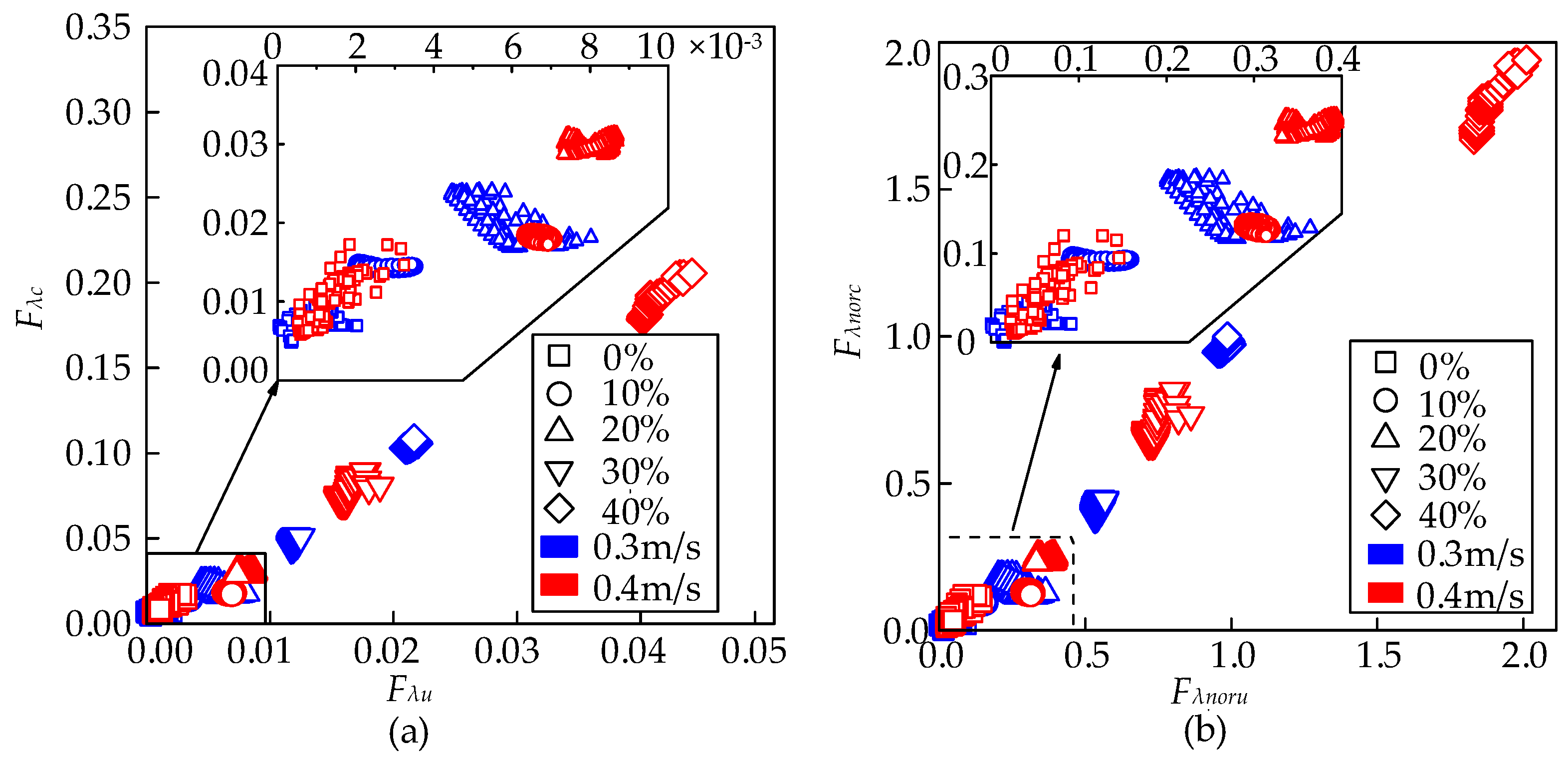
A time window with a length of 400 is applied to intercept the experimental data corresponding to 0.3 m/s shown in Figure 10. The time window is moved 100 time steps towards the right step by step. 100(time steps) × 5(severity levels of thrust loss) × 2(kinds of signal) sets of sample data are gotten. In the same way, another group of sample data corresponding to 0.4 m/s can be obtained. The TFE method is applied to extract fault features from the sample data, and the extracted fault features are normalized based on the RCQFFV. The results are shown in Figure 17.

As shown in Figure 17a, the percentage of thrust loss λ% increases from 0% to 40%, correspondingly, the fault feature extracted from surge speed, given the symbol F_λu, ranges from 0.00003 to 0.02197 for 0.3 m/s, from 0.00052 to 0.04416 for 0.4 m/s. Similarly, the fault feature extracted from the change rate of control voltage, given the symbol F_λc, ranges from 0.00479 to 0.10850 for 0.3 m/s, from 0.00583 to 0.20560 for 0.4 m/s. The results indicate that the range of one kind of fault feature is different from that of another kind of fault feature under the same working condition and that the distribution of one kind of fault feature obtained under one working condition is different from that of the same kind of fault feature obtained under another working condition.

In Figure 17a, the maximum and minimum of F_λu corresponding to 0.3 m/s are selected as $F_{\max }$ and $F_{\min }$ for normalization of F_λu. Similarly, the maximum and minimum of F_λc corresponding to 0.3 m/s are selected as $F_{\max }$ and $F_{\min }$ for normalization of F_λc. In Figure 17b, the F_λu normalized, given the symbol $F_{\lambda norc}$, and the F_λc normalized, given the symbol $F_{\lambda noru}$, range from 0 to 1 for 0.3 m/s. It indicates that different kinds of fault features have the same range after normalization for 0.3 m/s. The $F_{\lambda noru}$ ranges from 0.0223 to 2.01 and the $F_{\lambda norc}$ ranges from 0.0101 to 1.94 for 0.4 m/s. It indicates that different kinds of fault features have a different range after normalization for 0.4 m/s. In addition, the same kind of fault feature still has a different range after normalization under different surge speeds. The results indicate that the RCQFFV uses a single normalization scale to normalize the fault feature corresponding to different working conditions. When the single normalization scale matches the working condition, different kinds of fault features will have the same range after normalization. Otherwise, it doesn’t. Due to that one single normalization scale can only match one working condition, the same kind of fault feature still has a different range after normalization under different working conditions, making that there is still a distribution discrepancy of fault features.

(2)

Experimental validation of the MSN

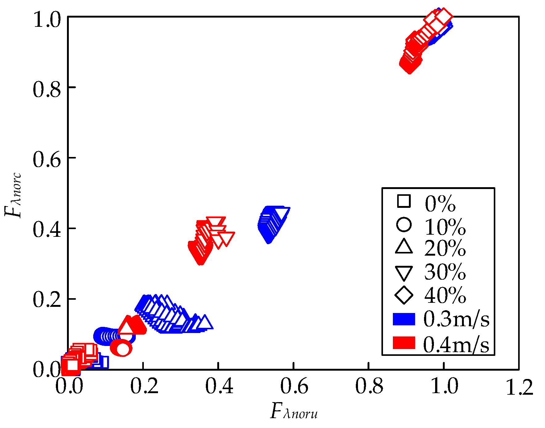
The fault features shown in Figure 17a are normalized based on the MSN. The results are displayed in Figure 18.

As shown in Figure 18, the fault features under different surge speeds all range from 0 to 1 after normalization based on the MSN. It indicates that the distribution discrepancy of fault samples under different surge speeds is reduced.

(3)

Experimental validation of the LSP

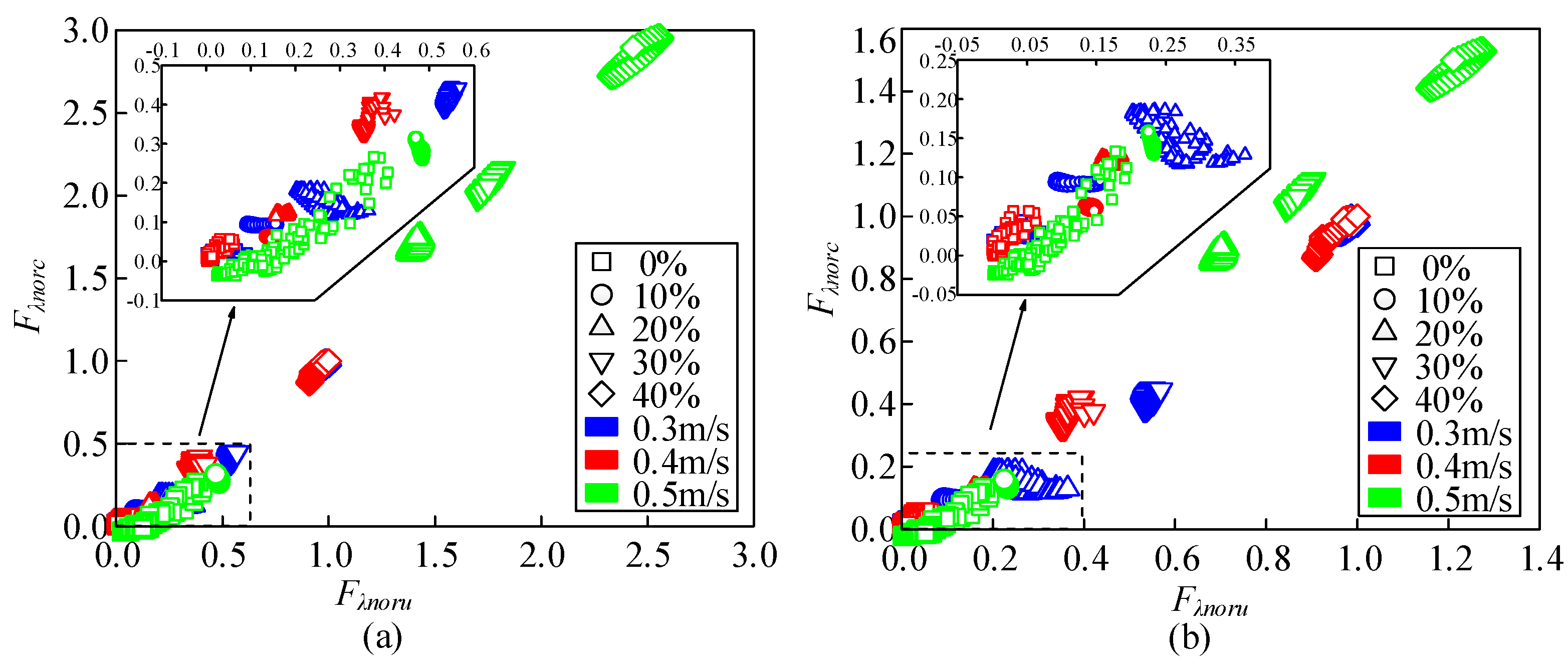
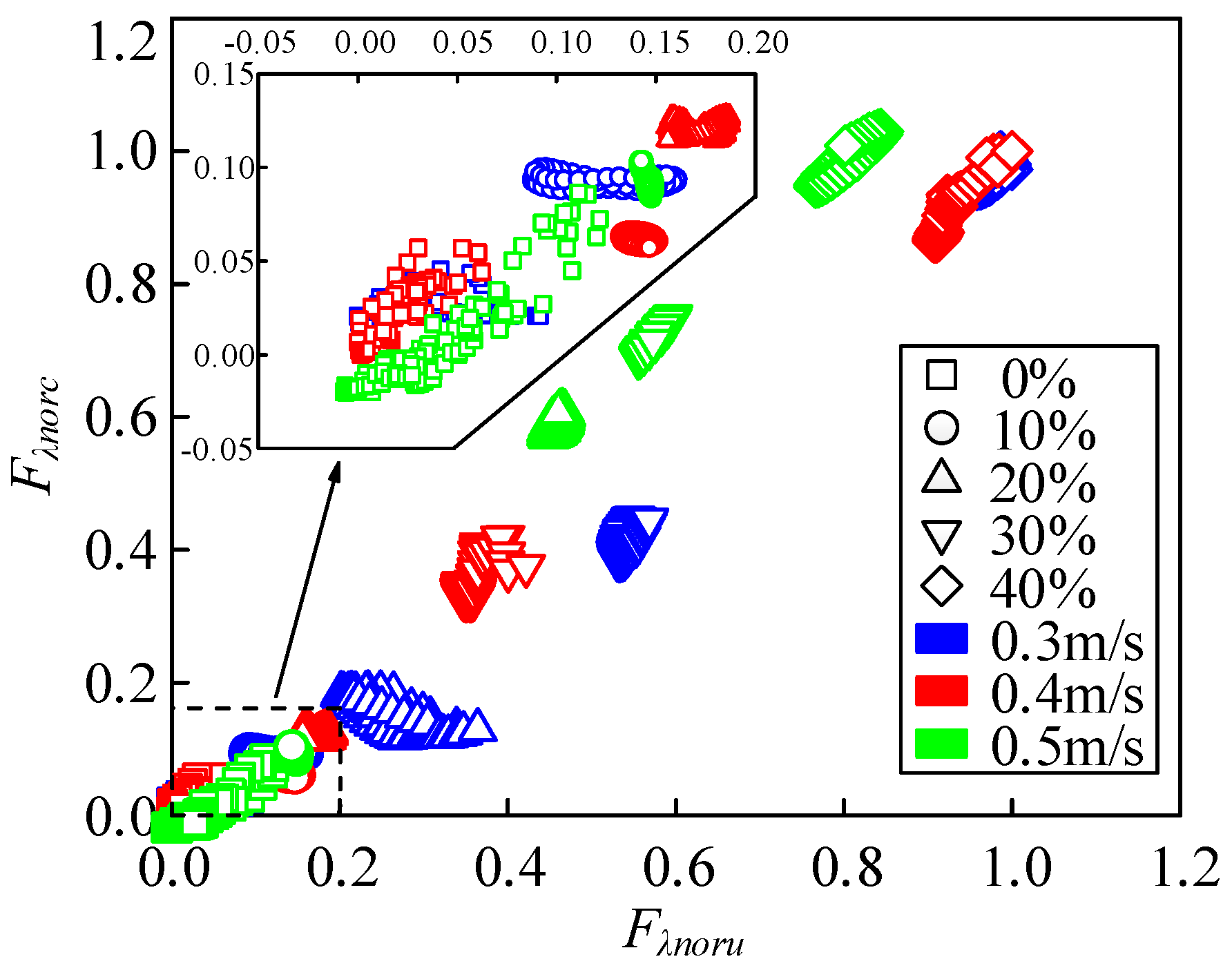
The fault features displayed in Figure 17a are selected as example features. In addition, fault features extracted from experiment data corresponding to 0.5 m/s are added to the example features. Assuming that the normalization scales are known for 0.3 m/s and 0.4 m/s, but it is unknown for 0.5 m/s. The example features are normalized by the MSN and the LSP. The results are displayed in Figure 19 and Figure 20.

In Figure 19a,b, the fault samples corresponding to 0.5 m/s are normalized by the normalization scale corresponding to 0.3 m/s and 0.4 m/s, respectively. It is shown that the distribution of fault samples for 0.5 m/s is quite different from the ones for 0.3 m/s and 0.4 m/s. Comparing Figure 20 with Figure 19, it is found that the distribution discrepancy of fault samples under different working conditions for the LSP is smaller than that for the MSN in the case of one working condition with no labeled training data.

(4)

Experimental validation of the TSVDD

According to experimental data obtained in Section 4.1, there are four working conditions, namely (A) 0.2 m/s, (B) 0.3 m/s, (C) 0.4 m/s, and (D) 0.5 m/s. Meanwhile, under each working condition, there are five severity levels of thrust loss, namely 0%, 10%, 20%, 30%, and 40%. For each severity level of thrust loss, there are two kinds of signals, namely the change rate of the control voltage for main thrusters and the surge speed of AUV. For each kind of signal, a time window with a length of 400 is applied to intercept the experimental data. The time window is moved 100 time steps towards the right step by step. 100 sets of sample data are gotten. The TFE method is applied to extract fault features from the sample data. The fault features corresponding to the same sample data constitute a fault sample. Half of the fault samples are used as training samples and the other half as testing samples. The training and testing sample sets are constructed as in

Table 1. Fault sample construction in experiment.

Working Condition	Surge Speed	Sample Type	0%	10%	20%	30%	40%
A	0.2 m/s	Training (number)	50	50	50	50	50
		Testing (number)	50	50	50	50	50
B	0.3 m/s	Training	50	50	50	50	50
		Testing	50	50	50	50	50
C	0.4 m/s	Training	50	50	50	50	50
		Testing	50	50	50	50	50
D	0.5 m/s	Training	50	50	50	50	50
		Testing	50	50	50	50	50

.

The methods SVDD, SVDD+RCQFFV, SVDD+RCQFFV+MSN, and SVDD+RCQFFV+MSN+LSP (namely the proposed TSVDD) are used to establish a classification model based on the training samples and to classify the testing samples. For convenience, detailed descriptions of the methods are given in the following. SVDD uses original fault samples to train and test the classification model. SVDD+RCQFFV, SVDD+RCQFFV+MSN, and proposed TSVDD use the fault samples normalized by RCQFFV, RCQFFV+MSN, and RCQFFV+MSN+LSP, respectively. The results are displayed in

Table 2. Diagnosis performance for the proposed TSVDD and other methods.

Case	SVDD	SVDD+RCQFFV	SVDD+RCQFFV+MSN	Proposed TSVDD
A→A	100	100	100	100
B→B	100	100	100	100
C→C	100	100	100	100
D→D	100	100	100	100
A→B①	28.4	37.6	37.6 (U)	37.6 (U)
A→B②			71.6 (B)	71.6 (B)
A→B③			20.0 (C)	65.2 (C)
A→B④			20.0 (D)	63.2 (D)
B→A①	40.0	31.2	31.2 (U)	31.2 (U)
B→A②			73.2 (A)	73.2 (A)
B→A③			20.0 (C)	62.0 (C)
B→A④			20.0 (D)	67.2 (D)
A→C①	24.8	28.8	28.8 (U)	28.8 (U)
A→C②			80.4 (C)	80.4 (C)
A→C③			40.0 (B)	72.0 (B)
A→C④			20.0 (D)	67.2 (D)
C→A①	23.2	28.0	28.0 (U)	28.0 (U)
C→A②			79.2 (A)	79.2 (A)
C→A③			40.0 (B)	75.2 (B)
C→A④			20.0 (D)	74.8 (D)
A→D①	26.0	24.0	24.0 (U)	24.0 (U)
A→D②			80.4 (D)	80.4 (D)
A→D③			54.4 (B)	74.4 (B)
A→D④			39.6 (C)	78.0 (C)
D→A①	24.0	26.0	26.0 (U)	26.0 (U)
D→A②			76.0 (A)	76.0 (A)
D→A③			24.8 (B)	68.0 (B)
D→A④			26.4 (C)	64.4 (C)
B→C①	36.0	35.6	35.6 (U)	35.6 (U)
B→C②			81.2 (C)	81.2 (C)
B→C③			32.8 (A)	75.6 (A)
B→C④			40.0 (D)	76.4 (D)
C→B①	41.2	38.8	38.8 (U)	38.8 (U)
C→B②			80.8 (B)	80.8 (B)
C→B③			31.6 (A)	76.4 (A)
C→B④			20.0 (D)	74.4 (D)
B→D①	34.0	30.8	30.8 (U)	30.8 (U)
B→D②			78.8 (D)	78.8 (D)
B→D③			28.4 (A)	72.4 (A)
B→D④			35.6 (C)	71.6 (C)
D→B①	32.0	29.2	29.2 (U)	29.2 (U)
D→B②			68.0 (B)	68.0 (B)
D→B③			20.0 (A)	63.2 (A)
D→B④			20.0 (C)	64.0 (C)
C→D①	38.0	26.4	26.4 (U)	26.4 (U)
C→D②			75.6 (D)	75.6 (D)
C→D③			21.2 (A)	58.8 (A)
C→D④			32.8 (B)	64.0 (B)
D→C①	26.0	28.0	28.0 (U)	28.0 (U)
D→C②			70.4 (C)	70.4 (C)
D→C③			19.6 (A)	58.0 (A)
D→C④			38.8 (B)	60.4 (B)

.

In transfer diagnosis case ‘A→A’, both the source and target datasets are A. The classification accuracy is 100% for the proposed TSVDD and the other three methods. It is also true in cases ‘B→B’, ‘C→C’, and ‘D→D’. It is reflected that both the proposed TSVDD and the other three methods have a good classification performance when the classification model is trained and tested under the same working condition.

In the transfer diagnosis case ‘A→B①’, the source dataset is A, and it contains sufficient labeled training data. The target dataset is B, and it includes unlabeled testing data. When the normalization scales of cases B, C, and D are unknown, the classification accuracy is 28.4% for the SVDD, while it is 37.6% for the methods SVDD+RCQFFV, SVDD+RCQFFV+MSN, and proposed TSVDD. It is reflected that both the proposed TSVDD and the other three methods have poor classification performance when only the normalization scale of the training dataset is known. Under the same conditions, in cases from ‘B→A①’, ‘A→C①’, to ‘D→C①’ listed in Table 2, the classification accuracy is 23.2–41.2% for the SVDD, while it is 24.0–68.8% for the other three methods. These results are consistent with the ones in case ‘A→B①’.

In transfer diagnosis case ‘A→B②’, when the normalization scale for working condition B is additionally known, the classification accuracy is 71.6% for the SVDD+RCQFFV+MSN and the proposed TSVDD. It is shown that the classification accuracy increases by 43.2%, 34.0%, and 0% using the proposed TSVDD compared with the SVDD, the SVDD+RCQFFV, and the SVDD+RCQFFV+MSN. It is reflected that the proposed TSVDD has the same classification accuracy as the SVDD+RCQFFV+MSN but has a higher one in comparison to the SVDD and the SVDD+RCQFF when the normalization scale of the target dataset is known. Under the same conditions, in cases from ‘B→A②’, ‘A→C②’, to ‘D→C②’ listed in Table 2, the classification accuracy increases 33.2–56.0%, 38.8–56.4%, and 0% using the proposed TSVDD compared with the other three methods, respectively. These results are consistent with the ones in case ‘A→B②’.

In transfer diagnosis case ‘A→B③’, when the normalization scale of working condition C is additionally known, the classification accuracy is 20.0% for the SVDD+RCQFFV+MSN, while it is 65.2% for the proposed TSVDD, showing that the classification accuracy increases 36.8%, 27.6%, and 45.2% using the proposed TSVDD compared with the SVDD, the SVDD+RCQFFV, and the SVDD+RCQFFV+MSN. In transfer diagnosis case ‘A→B④’. When the normalization scale of working condition D is additionally known, the classification accuracy is 20.0% for the SVDD+RCQFFV+MSN, while it is 63.2% for the proposed TSVDD, showing that the classification accuracy increases by 34.8%, 25.6%, and 43.2% using the proposed TSVDD compared with the other three methods, respectively. It is reflected that the proposed TSVDD has a higher classification accuracy when the normalization scale of the target dataset is unknown but the normalization scale of one other dataset is additionally known. It is also true in the other cases, namely in cases from ‘B→A③’ and ‘B→A④’ to ‘D→C③’ and ‘D→C④’ listed in Table 2, the classification accuracy increases 20.8–51.6%, 30.0–54.0%, and 20.0–54.8% using the proposed TSVDD compared with the other three methods, respectively.

The summary is as follows. If the source and target datasets are obtained under the same working condition, then both the proposed TSVDD and the other three methods have a good classification performance. If the source and target datasets are acquired under different working conditions, and only the normalization scale of the target dataset is known, then both the proposed TSVDD and the other three methods have poor classification performance. If the source and target datasets are gotten under different working conditions, and the normalization scale of the target dataset is additionally known, then the proposed TSVDD has the same classification accuracy as the SVDD+RCQFFV+MSN but has a higher one in comparison to the SVDD and the SVDD+RCQFF. If the normalization scale of the target dataset is unknown, but the normalization scale of one other dataset is additionally known, the classification accuracy for the proposed TSVDD is higher than the ones for the other three methods.

5. Conclusions

This article mainly investigates the severity level classification of fault samples of a thruster for AUVs under working conditions with no labeled training data. Since the fault feature extracted by the SPWVD is non-monotonic to fault severity, the TFE is proposed. Considering the SVDD has poor classification accuracy in the case that the classification model established under one working condition is transferred to another working condition, the TSVDD is proposed. The results of the pool experiments are presented as follows. The thruster fault causes the energy to migrate to a local region in the time-frequency power spectrum, forming an energy concentration. The greater the percentage of thrust loss, the stronger the energy concentration. The local region is closely surrounded by the time and frequency boundaries identified by the IPSE and the STNED. The sum of the energy in the boundaries contains little noise energy. It makes that the fault feature obtained by the TFE is monotonic to the percentage of thrust loss. There is a distribution discrepancy of fault samples under different working conditions. Due to the lack of normalization scale under the working condition with no labeled training data, a big distribution discrepancy still exists in the normalized fault samples. The TSVDD aligns the distribution of fault samples with the estimated normalization scale and makes the fault samples more suitable for classification. It leads that the TSVDD increases the classification accuracy by 20.8–51.6% compared with the SVDD under the working condition with no labeled training data.

References

1. Daqi, Z.; Huapeng, Z.; Chenxia, L. Tracking controller based on model prediction control for remotely operated vehicle for thruster fault. J. Mar. Sci. Technol. 2022, 27, 840–855. [Google Scholar]
2. Yeo, S.J.; Choi, W.S.; Hong, S.Y.; Song, J.H. Enhanced convolutional neural network for in Situ AUV thruster health monitoring using acoustic signals. Sensors 2022, 22, 7073. [Google Scholar] [CrossRef] [PubMed]
3. Hou, Z.; Li, X.G.; Wang, H.; Zhai, P.; Lu, H. Fuzzy linear extended states observer-based iteration learning fault-tolerant control for autonomous underwater vehicle trajectory-tracking system. IET Control Theory Appl. 2022. [Google Scholar] [CrossRef]
4. García-Molleda, D.; Sandoval, J.; Coria, L.N.; Bugarin, E. Energy-based trajectory tracking control for underwater vehicles subject to disturbances with actuator partial faults and bounded input. Ocean Eng. 2022, 248, 110666. [Google Scholar] [CrossRef]
5. Tian, Q.; Wang, T.; Liu, B.; Ran, G. Thruster fault diagnostics and fault tolerant control for autonomous underwater vehicle with ocean currents. Machines 2022, 10, 582. [Google Scholar] [CrossRef]
6. Wu, Z.; Wang, Q.; Huang, H. Adaptive neural networks trajectory tracking control for autonomous underwater helicopters with prescribed performance. Ocean Eng. 2022, 264, 112519. [Google Scholar] [CrossRef]
7. Cho, H.; Choi, H.-S.; Kim, H.-J.; Nam, K.S.; Ryu, J.D.; Ha, K.N. Feature selection for unmanned surface vehicle fault diagnosis research and experimental verification. J. Soc. Control Robot Syst. 2022, 28, 542–550. [Google Scholar] [CrossRef]
8. Chan, T.K.; Chin, C.S. Health stages diagnostics of underwater thruster using sound features with imbalanced dataset. Neural Comput. Appl. 2019, 31, 5767–5782. [Google Scholar] [CrossRef]
9. Capocci, R.; Omerdic, E.; Dooly, G.; Toal, D. Fault-tolerant control for ROVs using control reallocation and power isolation. J. Mar. Sci. Eng. 2018, 6, 40. [Google Scholar] [CrossRef] [Green Version]
10. dos Santos, C.H.; Cardozo, D.I.; Reginatto, R.; De Pieri, E.R. Bank of controllers and virtual thrusters for fault-tolerant control of autonomous underwater vehicles. Ocean Eng. 2016, 121, 210–223. [Google Scholar] [CrossRef]
11. Luca, P.; Marco, P.; Benedetto, A. A robust propulsion layout for underwater vehicles with enhanced manoeuvrability and reliability features. Proc. Inst. Mech. Eng. Part M-J. Eng. Marit. Environ. 2018, 232, 358–376. [Google Scholar]
12. Hao, L.Y.; Zhang, H.; Guo, G.; Li, H. Quantized sliding mode control of unmanned marine vehicles: Various thruster faults tolerated with a unified model. IEEE Trans. Syst. Man Cybern. Syst. 2021, 51, 2012–2026. [Google Scholar] [CrossRef]
13. Zhao, B.; Skjetne, R.; Blanke, M.; Dukan, F. Particle filter for fault diagnosis and robust navigation of underwater robot. IEEE Trans. Control Syst. Technol. 2014, 22, 2399–2407. [Google Scholar] [CrossRef] [Green Version]
14. Chaos, D.; Moreno-Salinas, D.; Aranda, J. Fault-tolerant control for AUVs using a single thruster. IEEE Access 2022, 10, 22123–22139. [Google Scholar] [CrossRef]
15. Huang, F.; Xu, J.; Yin, L.; Wu, D.; Cui, Y.; Yan, Z.; Chen, T. A general motion control architecture for an autonomous underwater vehicle with actuator faults and unknown disturbances through deep reinforcement learning. Ocean Eng. 2022, 263, 112424. [Google Scholar] [CrossRef]
16. Liu, F.; Tang, H.; Qin, Y.; Duan, C.; Luo, J.; Pu, H. Review on fault diagnosis of unmanned underwater vehicles. Ocean Eng. 2022, 243, 110290. [Google Scholar] [CrossRef]
17. Chu, Z.; Gu, Z.; Li, Z.; Chen, Y.; Zhang, M. A fault diagnostic approach based on PSO-HMM for underwater thrusters. Math. Biosci. Eng. 2022, 19, 12617–12631. [Google Scholar] [CrossRef]
18. Lei, Y.; Jia, F.; Kong, D.; Lin, J.; Xing, S. Opportunities and challenges of machinery intelligent fault diagnosis in big data era. J. Mech. Eng. 2018, 54, 94–104. [Google Scholar] [CrossRef]
19. Raanan, B.Y.; Bellingham, J.; Zhang, Y.; Kemp, M.; Kieft, B.; Singh, H.; Girdhar, Y. Detection of unanticipated faults for autonomous underwater vehicles using online topic models. Field Robot. 2018, 35, 705–716. [Google Scholar] [CrossRef] [Green Version]
20. Wang, J.; Wu, G.; Wan, L. Sensor fault diagnosis for underwater robots. In Proceedings of the 7th World Congress on Intelligent Control and Automation, Chongqing, China, 25–27 June 2008; Volume 12, pp. 254–259. [Google Scholar]
21. Sun, Y.S.; Ran, X.R.; Li, Y.M.; Zhang, G.C.; Zhang, Y.H. Thruster fault diagnosis method based on Gaussian particle filter for autonomous underwater vehicles. Int. J. Nav. Archit. Ocean Eng. 2016, 8, 243–251. [Google Scholar] [CrossRef] [Green Version]
22. Elhanaoui, A.; Aassif, E.; Maze, G.; Décultot, D. Time-frequency analysis to a particular type of scattering problems involving metallic-polymer tubing structures. Ultrasonics 2018, 82, 200–208. [Google Scholar] [CrossRef] [PubMed]
23. Abed, W.; Sharma, S.K.; Sutton, R.; Khan, A. An unmanned marine vehicle thruster fault diagnosis scheme based OFNDA. J. Mar. Eng. Technol. 2017, 16, 37–44. [Google Scholar] [CrossRef]
24. Jiang, Y.; Feng, C.; He, B.; Guo, J.; Wang, D.; Lv, P. Actuator fault diagnosis in autonomous underwater vehicle based on Neural Network. Sens. Actuators A Phys. 2021, 324, 112668. [Google Scholar] [CrossRef]
25. Wu, J.; Chen, X.; Ma, Z. A signal decomposition method for ultrasonic guided wave generated from debonding combining smoothed pseudo Wigner-Ville distribution and Vold–Kalman filter order tracking. Shock Vib. 2017, 2017, 529–541. [Google Scholar] [CrossRef] [Green Version]
26. Li, Y.; Liu, S.; Zhu, P.; Yu, J.; Li, S. Extraction of visual texture features of seabed sediments using an SVDD approach. Ocean Eng. 2017, 142, 501–506. [Google Scholar] [CrossRef]
Figure 1. The flow chart of the proposed TFE: (a) The schematic diagram; (b) The framework diagram.
Machines 10 01236 g001aMachines 10 01236 g001b
Figure 2. The schematic diagram of proposed IPSE.
Machines 10 01236 g002
Figure 3. The schematic diagram of proposed STNED.
Machines 10 01236 g003
Figure 4. The flow chart of the proposed TSVDD method: (a) The schematic diagram; (b) The framework diagram.
Machines 10 01236 g004
Figure 5. The schematic diagram of RCQFFV.
Machines 10 01236 g005
Figure 6. The schematic diagram of MSN.
Machines 10 01236 g006
Figure 7. The schematic diagram of LSP.
Machines 10 01236 g007
Figure 8. Physical layout of the AUV.
Machines 10 01236 g008
Figure 9. The waveform of the experimental data.
Machines 10 01236 g009
Figure 10. The selected experimental data: (a) The surge speed of AUV; (b) The change rate of the control voltage for main thrusters.
Machines 10 01236 g010
Figure 11. The time-frequency power spectrums of the example data: (a) λ% = 0%; (b) λ% = 10%; (c) λ% = 20%; (d) λ% = 30%; (e) λ% = 40%.
Machines 10 01236 g011
Figure 12. The instantaneous power spectrum entropy curves corresponding to different percentages of thrust loss: (a) λ% = 10%; (b) λ% = 20%; (c) λ% = 30%; (d) λ% = 40%.
Machines 10 01236 g012
Figure 13. The time boundaries of the local region identified by the IPSE: (a) λ% = 10%; (b) λ% = 20%; (c) λ% = 30%; (d) λ% = 40%.
Machines 10 01236 g013
Figure 14. The energy difference curves corresponding to different percentages of thrust loss: (a) λ% = 10%; (b) λ% = 20%; (c) λ% = 30%; (d) λ% = 40%.
Machines 10 01236 g014
Figure 15. The frequency boundaries of the local region recognized by the STNED: (a) λ% = 10%; (b) λ% = 20%; (c) λ% = 30%; (d) λ% = 40%.
Machines 10 01236 g015
Figure 16. The fault features extracted from different signals under various working conditions: (a) The surge speed at 0.3 m/s; (b) The surge speed at 0.2 m/s; (c) The surge speed at 0.4 m/s; (d) The surge speed at 0.5 m/s; (e) The change rate of the control voltage at 0.2 m/s; (f) The change rate of the control voltage at 0.3 m/s; (g) The change rate of the control voltage at 0.4 m/s; (h) The change rate of the control voltage at 0.5 m/s.
Machines 10 01236 g016
Figure 17. The distribution of the fault samples normalized by the RCQFFV: (a) Original fault samples; (b) Normalized fault samples.
Machines 10 01236 g017
Figure 18. The distribution of the fault samples normalized by the MSN.
Machines 10 01236 g018
Figure 19. The distribution of the fault samples normalized by the MSN under working condition with no labeled training data: (a) The normalization scale corresponding to 0.3 m/s; (b) The normalization scale corresponding to 0.4 m/s.
Machines 10 01236 g019
Figure 20. The distribution of the fault samples normalized by the LSP.
Machines 10 01236 g020