Article

Research on the Gearbox Fault Diagnosis Method Based on Multi-Model Feature Fusion

1
School of Mechanical Electrical and Vehicle Engineering, East China Jiaotong University, Nanchang 330013, China
2
State Key Laboratory of Performance Monitoring Protecting of Rail Transit Infrastructure, East China Jiaotong University, Nanchang 330013, China
*
Author to whom correspondence should be addressed.
Machines 2022, 10(12), 1186; https://doi.org/10.3390/machines10121186
Submission received: 8 November 2022 / Revised: 6 December 2022 / Accepted: 7 December 2022 / Published: 8 December 2022
(This article belongs to the Section Machines Testing and Maintenance)

Abstract

:
The gearbox is an important component of rotating machinery and is of great significance for gearbox fault diagnosis. In this paper, a gearbox fault diagnosis model based on multi-model feature fusion was proposed that addressed the limitations of a single or few features reflecting the gearbox’s fault state. The time–frequency feature of the vibration signal was extracted, and the sensitive feature was selected. The sensitive features were extracted using a one-dimensional convolutional neural network. The parallel fusion method was used to fuse the two domain features as inputs to the support vector machine model. The radial basis kernel function and penalty factor of the support vector machine were optimized by improving the particle swarm optimization algorithm. Finally, the gearbox states were identified using the optimized support vector machine model. The results show that the recognition rate of the proposed model is 98.3%, which is higher than that of other models.

1. Introduction

Gearboxes are widely used in mechanical equipment due to their role in power transmission [1,2]. The working environment of a gearbox is relatively harsh, and various faults often occur during operation, which affects the working state of the gearbox and can cause heavy casualties and economic losses [3,4].
Research on gearbox faults began in the early 20th century. By 1968, gearbox fault diagnosis became an important standard for determining whether gear performance met the requirements, and it attracted the attention of many scholars worldwide [5,6]. Bao et al. [7] described the mathematical model of the faulty gear vibration signal in 1992 and verified the effectiveness of diagnostic methods such as broadband demodulation technology, correlation spectrum analysis, and refined complex envelope analysis. Wang et al. [8] proposed resonance demodulation, wavelet analysis, and model-based autoregressive diagnostic methods in 1999. Wu et al. [9] proposed a gear fault diagnosis and feature-extraction method and analyzed and extracted the time–frequency characteristics of gear failure vibration signals. The experimental results indicated that the proposed method had a higher recognition rate. Some recent studies have focused on the classification of dynamic data distribution using different algorithms. Cao et al. [10] presented a novel intelligent technique for tool-wear state recognition using machine spindle vibration signals. Additionally, that study combined derived wavelet frames and a convolutional neural network. ND et al. [11] proposed condition monitoring of a face milling cutting tool with the help of Artificial Neural Network based multilayer perceptron approach. The results confirmed that multilayer perceptron approach provides more classification accuracy.
Because time–frequency domain feature selection was successful in the gearbox fault diagnosis, its integration with machine learning is the next step to consider. Some machine learning algorithms are being used in gearbox fault diagnosis [12,13]. Wang et al. [14] proposed a data-driven fault diagnosis method for wind turbine gearboxes, which was based on three models: a gray wolf optimized variational mode decomposition method (AGWO-VMD), normalized composite multiscale dispersion entropy (NCMDE), and a long short-term memory network (LSTM) [15]. Recently, neural-network techniques have been used for fault diagnosis. Khalil et al. [16] used a fast Fourier transform (FFT) to obtain the fault frequency signature and principal component analysis (PCA) to obtain the most important data with reduced dimensions. The proposed method was validated using two circuits. Khalil et al. [17] proposed self-healing to recover a faulty embryonic cell through the innovative usage of healthy cells, and the researchers achieved a high-accuracy fault prediction with a low training time. However, when faced with multiple data samples, these shallow learning models often led to poor prediction results due to factors such as insufficient model generalization ability [18].
The deep learning model has the functions of feature extraction and pattern recognition, which can reduce the dependence on signal processing technology in the fault diagnosis process [19,20]. In addition, because of its powerful representation ability, it can meet the current industrial big data development requirements [21]. Deep learning models have been developed to address the issues with gearboxes, such as convolutional neural networks (CNN) [22,23], deep belief networks (DBN) [24], and generative adversarial neural networks (GAN) [25]. Wu et al. [26] used a one-dimensional convolutional neural network (1DCNN) model to analyze the original vibration signal in the process of tank gearbox fault diagnosis, and the results showed that the 1DCNN model can effectively identify the fault state of the tank gearbox. Zhang et al. [27] extracted sensitive features using a 1DCNN and verified its effectiveness. Research on various intelligent algorithms has evolved to the point where fault diagnosis is no longer limited to a specific algorithm [28]. Multi-model fusion methods also play an important role in fault diagnosis [29]. Currently, the commonly used multi-model fusion techniques can be divided into three methods: data layer fusion, feature layer fusion, and decision layer fusion [30]. Although the aforementioned fault diagnosis methods can correctly diagnose gearbox faults in most cases, the multi-model fusion method can be improved.
A gearbox fault diagnosis model based on multi-model feature fusion was proposed in this study. The contributions of this study are as follows.
(1)
Eight time–frequency sensitive features are extracted and selected. The 1DCNN was used to extract the original vibration signal features.
(2)
The parallel fusion method was used to fuse the two domain features as the input of the support vector machine (SVM) model.
(3)
The improved particle swarm optimization (IPSO) algorithm is used to optimize the SVM classifier to achieve gearbox fault diagnosis and obtain more accurate and effective results.
The remainder of this paper is organized as follows. Section 2 introduces the gearbox fault diagnosis background, including the 1DCNN, SVM, IPSO, and feature fusion. Section 3 introduces the experimental platform construction and data collection. Section 4 introduces the construction of the fault diagnosis model. In Section 5, the experimental results are analyzed and verified. Section 6 concludes the paper and discusses future work.

2. Background

2.1. 1DCNN

Convolutional neural networks (CNN) were first proposed by Sercu et al. [31]. Neural network models can be used to document and identify images. This model can directly process two-dimensional images through weight-sharing and convolution operations. It can also avoid the tedious feature extraction and data reconstruction processes involved in traditional intelligent algorithms. The 1DCNN model is a feed-forward neural network and supervised learning model; that is, the input sample needs the corresponding sample label for supervised learning, which is usually composed of a convolutional layer, pooling layer, fully connected layer, and a softmax classifier. It is necessary to select the appropriate activation function, optimizer, and learning rate.
The main function of the convolutional layer is to continuously extract features from the previous layer’s data by setting the size of the convolution kernel [32]. Weight sharing is the main characteristic of the convolutional layers. Weight sharing can effectively reduce the parameters required in the training process, accelerate the model training, and reduce the occurrence of overfitting. The expression for the convolution operation is as follows:
x j l = f ( i m j x i l 1 k i j l + b j l ) ,
where l is the lth convolutional layer, x j l is the lth layer output, x i l 1 is the lth layer input, k i j l is the weight matrix, b j l is the bias, f ( ) is the activation function, and m j is the ( l 1 ) th convolutional region of the layer feature map [33].
In the 1DCNN structure, the pooling layer mainly performs pooling processing through the images extracted from the convolutional layer, which can significantly reduce the number of calculations during the model operation and reduce the occurrence of overfitting [34]. Pooling methods include mean pooling, max-pooling, and stochastic pooling. This study adopted the max-pooling method to reduce the feature errors. The general calculation process for pooling is as follows:
X j l = f ( β j l d o w n ( X j l 1 ) + b j l ) ,
where β j l and b j l are the multiplicative and additive biases of the lth neuron of the jth layer network, respectively, and d o w n ( ) represents the sampling function.
The main task of the fully connected layer in the 1DCNN model is to summarize the local features extracted by the convolutional and pooling layers. After the local features were fused by the fully connected layer, they were identified using a softmax classifier.

2.2. IPSO

Based on the traditional PSO algorithm, the improved particle swarm optimization (IPSO) utilizes the adaptive inertia weight and population shrinkage factor to speed up convergence and improve the search accuracy. This is performed to address the PSO algorithm’s problem of falling into the local optimal solution (and thereby affecting the search) [35]. In the PSO algorithm, when the value of the weight ω is large, the particle has a strong ability to move in the solution space. Thus, the search ability in the global scope is also relatively strong. When ω is small, the ability of the particle to search for the optimal solution in the local area is strengthened, making it easier for the algorithm to converge. In the traditional PSO algorithm, setting a fixed value of ω easily leads to the setting of ω being too large, which causes the PSO algorithm to converge prematurely during the running process. If it is too small, the model will easily fall into the local optimum, and the expected search effect will not be achieved. The weight of the PSO algorithm selects a relatively large ω at the beginning of the iteration, which not only ensures that the algorithm has a powerful global search ability, but also has the ability to jump out of the local optimum. In the later stages of the iteration, using a smaller ω for a stronger local search is beneficial for the convergence of the algorithm [36]. In this study, ω is expressed by Equation (3):
ω = { ω min ( ω max ω min ) × ( f f min ) f a v g f min f f a v g ω max f > f a v g ,
where f represents the function value of the objective function optimized in the current PSO; ωmax and ωmin are the maximum and minimum values of the inertia weight factor, respectively; and fmin and favg are the minimum and average values of the particle objective function values, respectively.
Equation (3) shows that, when f tends to be consistent or tends toward a local optimal solution, ω in the PSO algorithm increases, and when each f is relatively scattered, ω decreases. When the f of the particle is better than favg, its corresponding ω will be smaller; thus, the particle is preserved. Conversely, when the f of the particle is worse than favg, the corresponding ω of the particle will be larger, making the particle move closer to a better search area. If the diversity of the population gradually decreases during the calculation process of the PSO algorithm, the population will be far from the global optimal position, which is equivalent to implementing the “diffusion” operation on the population. If the diversity of the population gradually increases, the population continues to approach the global optimal position, which is equivalent to an “attraction” operation on the population [37]. To address this problem, this study introduces a shrinking factor based on the adaptive weight factor, and its calculation expression is shown in Equation (4):
ω = 2 | 2 C C 2 4 C | C = c 1 + c 2   C > 4 ,
where C is the balance factor, and c1 and c2 are the learning factors. Clerk et al. [38] proposed that when C = 4.1, the species diversity of PSO can be maintained and the convergence ability is better. Here, ω = 0.7298, and the population speed update is as follows:
v i = ω ( w v i + c 1 r 1 ( P i x i ) + c 2 r 2 ( G i x i ) ) ,
where vi is the particle velocity, ri is a random number between (0, 1), Pi is the global optimal particle, Gi is the individual optimal particle, and xi is the current position of the particle.

2.3. SVM

As a data analysis method developed based on statistical learning theory, SVM can solve data processing problems, such as regression problems and pattern recognition, and can also be extended to fields and disciplines such as prediction and comprehensive evaluation [39,40,41,42]. The SVM model was originally applied to binary classification, that is, to find a hyperplane to separate the positive and negative categories that need to be classified. Simultaneously, two parallel hyperplanes with as large intervals as possible were constructed on each side to ensure a good classification ability. The error generalization ability of the SVM increased as the distance between the two hyperplanes increased. The support vector was the training sample closest to the hyperplane and was the basis of the classification func-tion used to form classification [43].
In the process of classifying nonlinear data using an SVM, the mapping of the input data to a high-dimensional space was completed using a kernel function. The selection of different kernel functions affected the classification. Cheng et al. [44] demonstrated that the radial basis kernel function has a wider application range than polynomial and sigmoid functions do. Therefore, the radial basis kernel function was selected for this study, and its mathematical expression is as follows:
K ( x , x k ) = exp [ x x k 2 2 σ 2 ] ,
where x is the n-dimensional input vector, x k is the center of the radial basis kernel function, x x k is the norm of x x k , and σ is the standard kernel function parameter [45].
Due to the fact that the SVM itself can only deal with binary classification problems, the multi-classification SVM model decomposes multi-classification problems into multiple binary classification problems. The multi-classification SVM model used in this study is the one-against-all SVM. The goal of the one-against-all SVM algorithm is that each support vector machine established can separate the data of one category from the data of other categories. In this method, one class in the dataset is regarded as the “+1” class, and the rest are regarded as the “−1” class. The first SVM model was then established. One class was separated from all the remaining classes, and the iteration was performed until all classes were separated pairwise. If the number of categories in a dataset is M, then the method must establish an SVM classifier using M. A flowchart of pattern recognition using a four-class SVM is shown in Figure 1.

2.4. Feature Fusion

Serial and parallel fusions are the most commonly used feature-level fusion methods. The serial and parallel fusion methods are shown in Equations (7) and (8), respectively:
d 1 = [ n 1 × e , n 2 × f ] ,
d 2 = [ ( n 1 × e ) + ( n 2 × f ) ] ,
where n1 and n2 are the weights of feature vectors e and f, respectively, if the dimensions of these two feature vectors are g and h, respectively. The fusion feature d1 can be obtained from Equation (7), and the dimension of the feature vector d1 after serial fusion is (g + h), as shown in Equation (8). Similarly, n1 and n2 are the weights of the feature vectors e and f, respectively, and the dimensions of these two feature vectors are the g-dimension and h-dimension, respectively. The dimension of the feature vector d2 fused by the parallel fusion method is the same as the dimension of the highest dimension of the feature vectors e and f.
From the above introduction of these two fusion methods, it can be seen that series fusion involves directly and simply splicing feature vectors, whereas parallel fusion fuses feature vectors that need to be fused using a fusion algorithm. Serial fusion has problems, such as increasing the dimension of the fusion feature vector and causing the information conflict of the feature vector, whereas parallel fusion does not increase the dimension of the fusion feature vector after fusion is performed by the relevant algorithm. Moreover, studies have shown that the parallel fusion method performs better than the serial fusion method in practical applications [46]. Therefore, the parallel fusion method was adopted to fuse the feature set in this paper, and its mathematical expression (9) is as follows:
d i = ( e i ) 2 + ( f i ) 2
If the dimensions of the two feature sets to be fused are not equal, the low-dimensional feature set must be complemented by zero.

3. Experimental Platform Construction and Data Collection

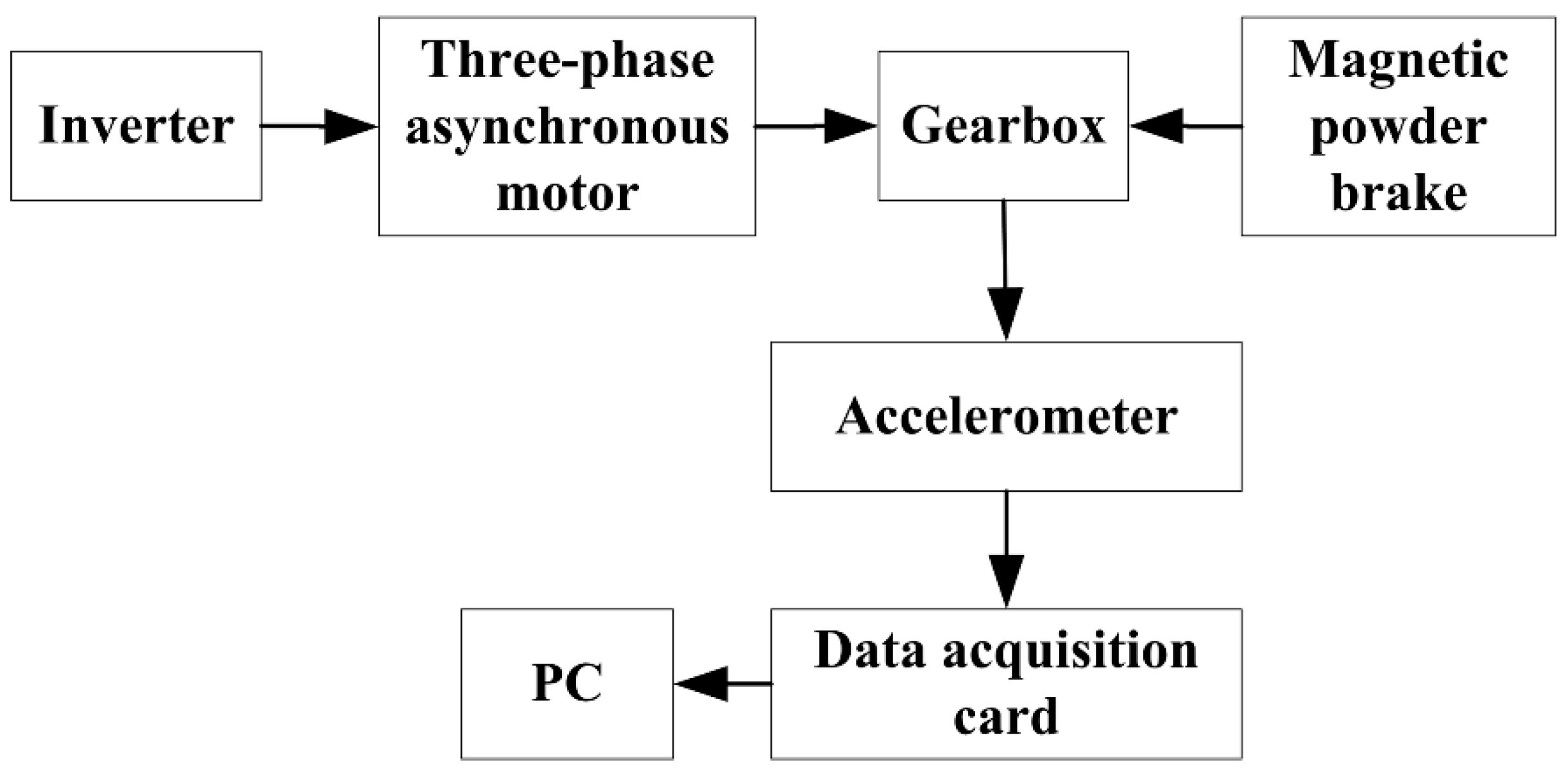
To verify the effectiveness of the proposed method for recognizing the fault state of a gearbox, an experimental scheme for the fault diagnosis of a gearbox was designed using frequency converters, motors, gearboxes, magnetic powder brakes, piezoelectric accelerometers, data acquisition cards, and a PC. A three-phase asynchronous motor (model YE2-100L2-4) was selected, and the frequency converter model was G7R5/P011-T4, which means that the operation of the frequency conversion and speed regulation of the three-phase asynchronous motor was completed. The gearbox model used was JZQ250; its reduction ratio is 10.35, and the output speed is 0~145 rpm. The magnetic powder brake model FZ-A-12 was selected. The vibration data were collected using a YE6231 data-collection system produced by Jiangsu Lianneng Electronic Technology Co., Ltd. The CAYD051V piezoelectric accelerometer, whose sensitivity is 100 mV/g, was selected for the acquisition of vibration signals, because it has the characteristics of a strong anti-interference ability, wide measurement range, and wide frequency range. The connection diagram of the experimental device and physical chart of the platform are shown in Figure 2 and Figure 3, respectively.
The construction process of the gearbox fault diagnosis experimental platform is as follows.
(1)
To ensure safety during the experiment, an air switch was installed between the power plug and inverter.
(2)
The inverter was connected to the motor, and the motor and gearbox were connected through the belt. The gearbox and the magnetic powder brake were connected through the coupling, and the motor, gearbox, and magnetic powder brake were fixed in the base plate.
(3)
A piezoelectric accelerometer was installed at the axial position of the bearing cover of the high-speed shaft of the gearbox, and the sensor, acquisition card, and PC were connected through the signal output line.
(4)
Four types of vibration data were obtained from the experiment: normal, wear, pitting, and broken gears. The motor speed was set at 900 rpm, and the sampling frequency was set at 6 kHz. A total of 1.8 million data points were collected for each state. The data groups, data length, sampling frequency, and motor speed of the vibration data obtained from the experiments are listed in Table 1.

4. Fault Diagnosis Model Construction

4.1. 1DCNN-IPSO-SVM Model

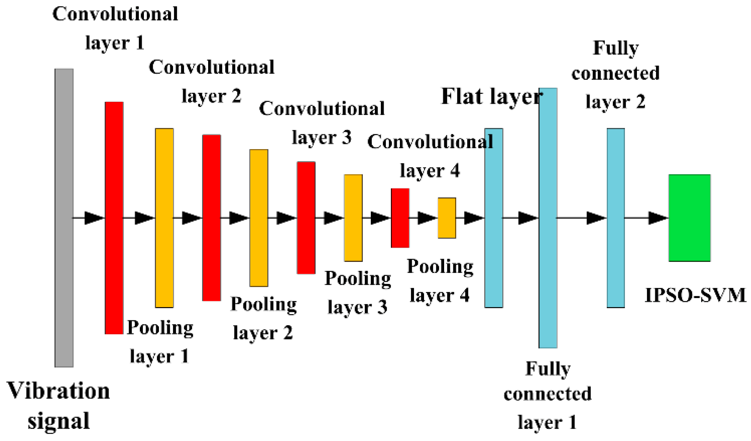
The overall workflow of the 1DCNN-IPSO-SVM model is shown in Figure 4. The 1DCNN model parameters are shown in Table 2. The first step is to input the collected one-dimensional vibration data into the established 1DCNN model, and the convolution function then selects a one-dimensional convolution function. During training, the Adam algorithm was selected to optimize the loss function, the learning rate was set to 0.001, and the activation function of each layer of the model was set to the rectified linear unit (ReLU) function. The ReLU is an unsaturated nonlinear function, which can be guaranteed to be positive in the calculation. To prevent the model from overfitting, a dropout layer was introduced, with the dropout = 0.8. The epoch size was set to 30, and the batch size was set to 20. As there were 6000 sets of experimental sample data, including 4800 sets of training samples and 1200 sets of test samples, each epoch had 160 training steps. A trained model was obtained after each training epoch. The model fit was obtained by substituting the training and validation data into the trained model. The second step was to run the model ten times, select the model with the highest accuracy, and maintain the network structure and parameters. Feature extraction was then performed, and the feature samples were used as input samples for the IPSO-SVM algorithm to obtain recognition results.

4.2. Multi-Model Feature Fusion Fault Diagnosis Model Framework

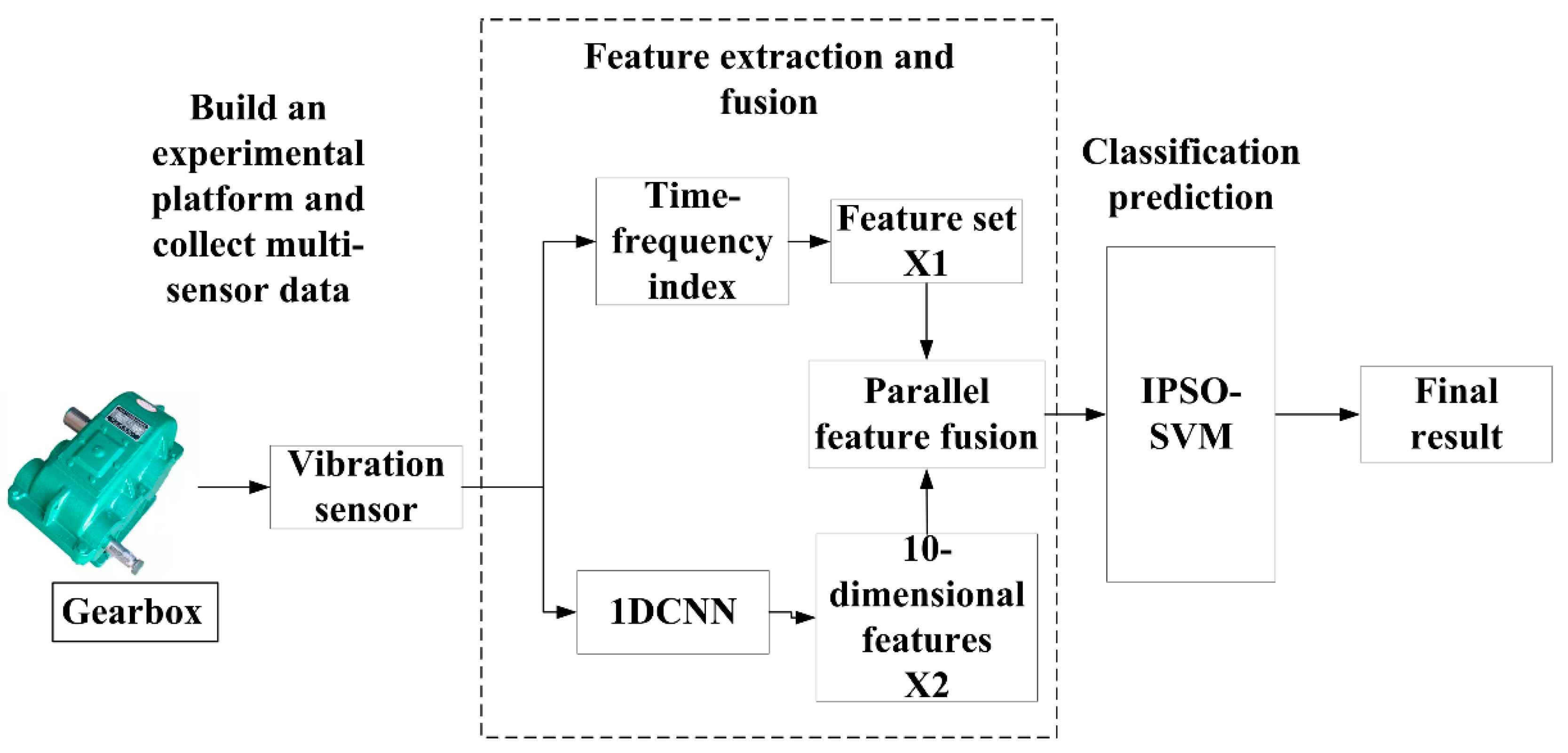
Multi-model fusion is a multi-model combination and integration, which is a method of combining multiple models in some way [47]. It seeks a better model to solve complex problems through multi-model fusion technology. The model-fusion strategy can be divided into three levels: sensor, feature, and decision level fusion [46]. In this study, a feature-level fusion strategy was used for feature fusion. The specific process of the gearbox fault diagnosis model framework based on multi-model feature fusion is shown in Figure 5.
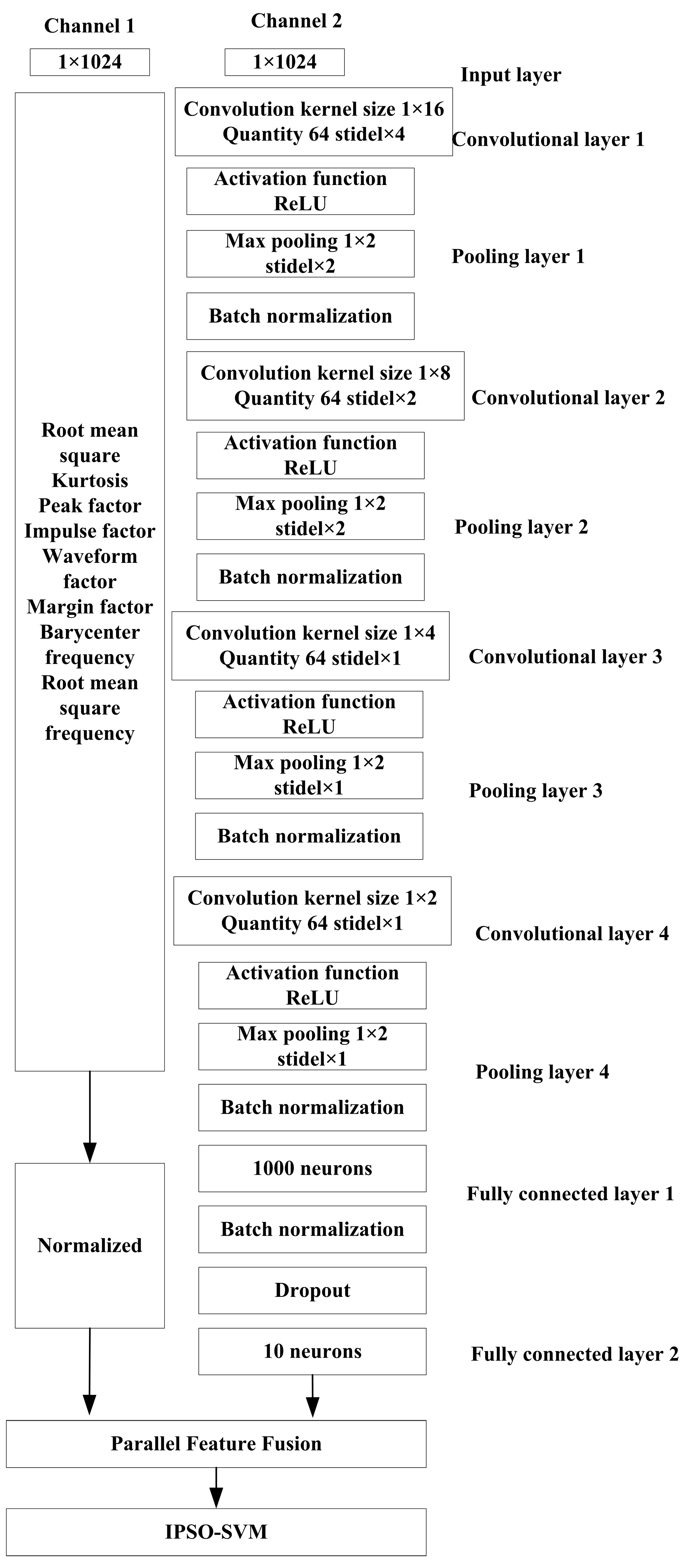
As is shown in Figure 5, the vibration data of each state of the gearbox were obtained through vibration sensors, and the obtained data were subjected to time–frequency domain feature extraction and 1DCNN model feature extraction. The feature sets {X1} and {X2} were fused using the parallel fusion method. Finally, the IPSO-SVM model was used to complete the fault recognition of the gearbox. The specific parameters of the gearbox fault diagnosis model of the multi-model feature fusion are shown in Figure 6.
To compress the length of the original vibration data and fully extract useful information, the number and size of the convolution kernels of the 1DCNN models were reduced. As shown in Figure 6, the parameters of each layer of the gearbox fault diagnosis model with multi-model feature fusion were obtained, and each group of 1024-long experimental vibration signals was processed using four convolution layers, four pooling layers, and two full connection layers to obtain ten-dimensional feature samples. The selection of the time–frequency domain parameters mainly included the root mean, kurtosis, peak factor, impulse factor, wavelet factor, margin factor, barycenter frequency, and root mean square frequency. Fusion was conducted using feature fusion technology to complete the pattern recognition.

5. Experimental Analysis and Verification

5.1. Time–Frequency Domain Feature Extraction

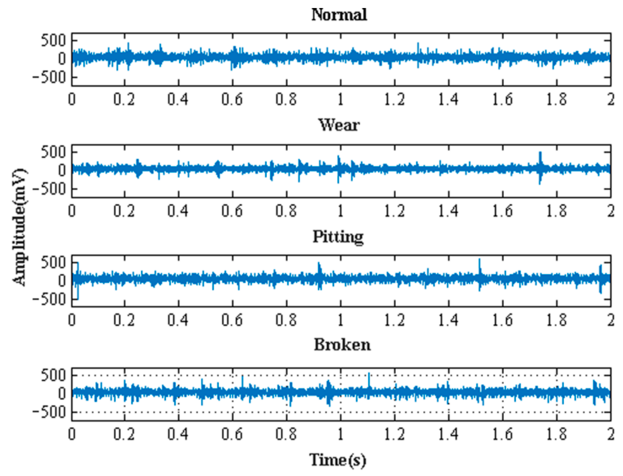
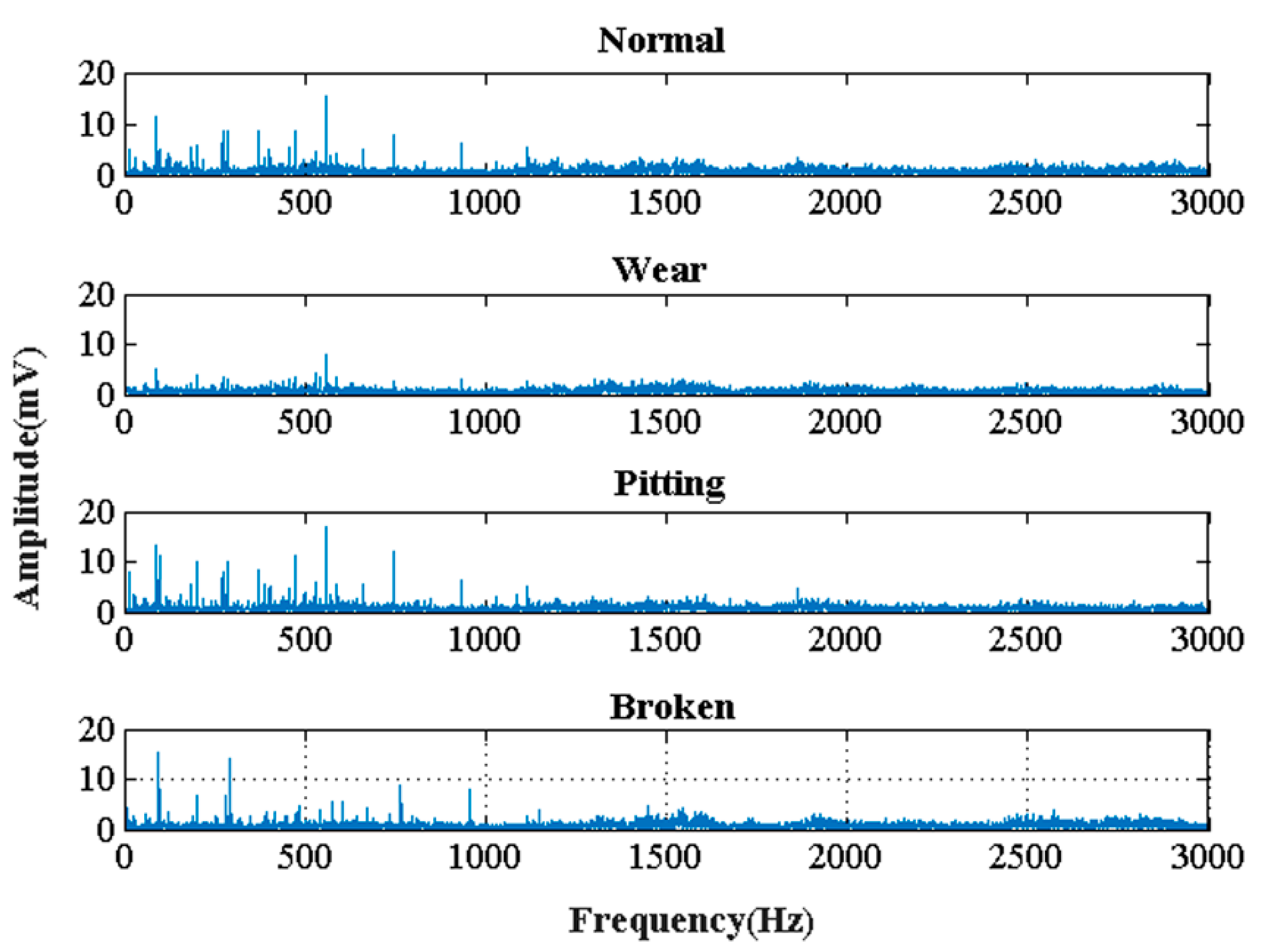
Using the experimental parameters in Table 1 and the no-load condition, the time–domain and frequency–domain diagrams of the experimental data of the four gearbox states were obtained, as shown in Figure 7 and Figure 8, respectively.
Figure 7 and Figure 8 show that the time–frequency characteristics of the four states are significantly different. In this study, after the complete ensemble empirical mode decomposition with adaptive noise (CEEMDAN) joint wavelet threshold denoting of the gearbox vibration data [48], eight time–frequency domain features were selected: root mean square (RMS), kurtosis, peak factor, impulse factor, waveform factor, margin factor, barycenter frequency, and RMS frequency. The root mean square (RMS) and kurtosis are dimensional time–domain indicators that reflect the vibration amplitude and energy change, respectively. The peak, impulse, waveform, and margin factors are dimensionless time–domain indicators that reflect the distribution of the vibration time series. The barycenter frequency and root mean square frequency are frequency–domain indicators that reflect changes in the position of the main frequency band. The calculation equations for the eight time–frequency and characteristic indicators are listed in Table 3.
In the eigenvalue calculation, the abovementioned eight time–frequency domain eigenvalues are very different, and the new features obtained using Equation (9) to fuse the features have a limited degree of distinction. Therefore, the time–frequency domain features of the vibration data were first normalized and then fused using Equation (9). The calculation process for the normalization operation is given by Equation (10):
Z = z min max min ,
where max and min are the maximum and minimum values of the sample data, respectively, and the data can be mapped to the interval [0, 1]. Table 4 lists the normalized eigenvalues of the samples. According to Equation (9), two sets of feature sets are complemented by zero. Eight time–frequency domain features and two complemented features are combined into the feature set {X1}.

5.2. Feature Extraction Analysis

Using the experimental parameters in Table 1 and the no-load condition, the vibration data of the four gearbox states were obtained. The vibration data of the four gearbox states were extracted using the 1DCNN model, and eight groups of ten-dimensional feature samples were obtained to form the feature set {X2}. The specific features are listed in Table 5.
Feature sets {X1} and {X2} were fused using the parallel fusion method. Some fused feature data are shown in Table 6.
Table 6 lists the eigenvalues obtained after the fusion of {X1} and {X2}. Using this method, the feature extraction of the original vibration data was completed, and feature set {D} was obtained by feature fusion, which was used for the next state recognition.

5.3. IPSO-SVM Parameter Analysis

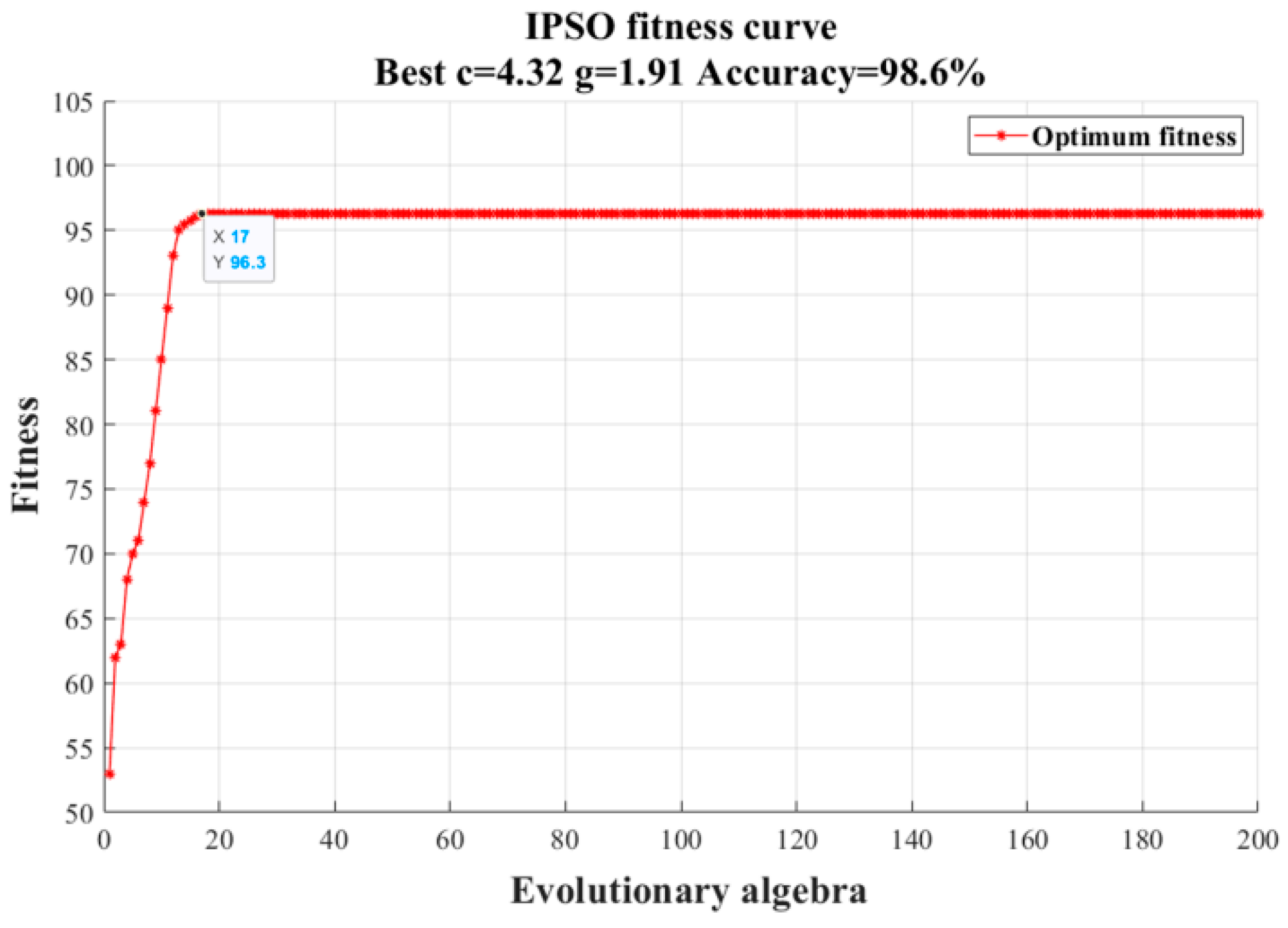
After the feature sets {X1} and {X2} were fused in parallel, a 6000 × 10-dimensional feature set {D} was obtained and used as the input sample for the IPSO-SVM model. The training and test datasets were divided according to a ratio of 8:2, that is, 1200 sets of training samples for each state for a total of 4800 sets of training samples. Totals of 300 test sets for each state and 1200 test sets were obtained. The initial parameters of the SVM were set as learning factors c1 = 1.8, c2 = 2.3, initialized maximum weight ωmax = 0.9, initialized minimum weight ωmin = 0.4, number of particles = 30, and number of iterations = 200. The IPSO-SVM fitness curves are shown in Figure 9.
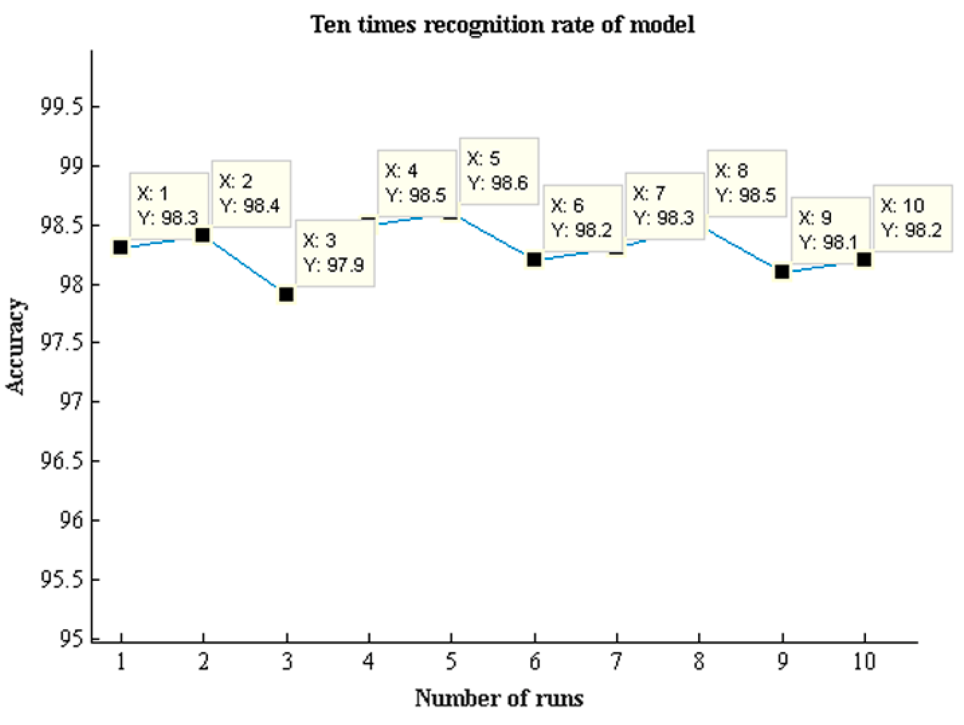
After the SVM model was optimized using the IPSO algorithm, the best-fitness-change curve was obtained, as shown in Figure 9. Figure 9 also shows that the IPSO-SVM model has the best fitness value of 96.3 after 17 iterations; it does not fall into the local optimum, and the convergence speed is fast. The recognition rate was 98.6%, the optimal penalty factor C was 4.32, and the kernel parameter γ was 1.91. To prevent the contingency in the classification recognition experiment and verify the reliability of the model, the IPSO-SVM model was run 10 times; the recognition accuracy of the 1200 test sets is shown in Figure 10, where the recognition accuracy refers to the ratio between the correct number of test samples and the total test samples.
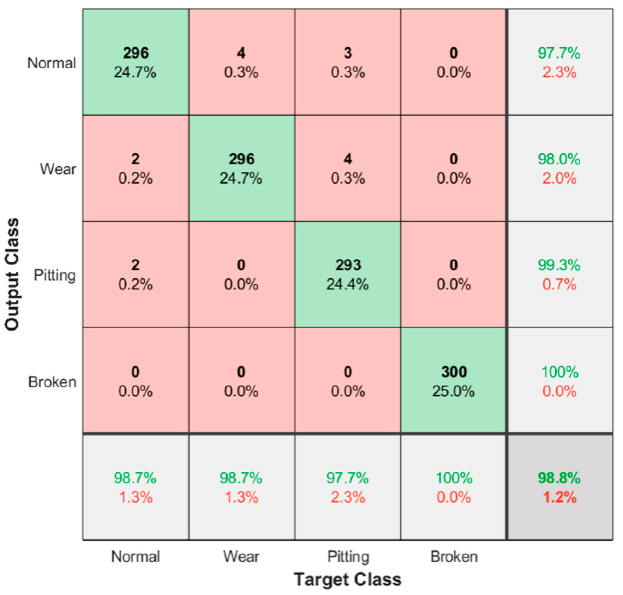
As shown in Figure 10, the average recognition accuracy of the model running 10 times was 98.3%, of which the highest was the fifth time, and its recognition accuracy was 98.6%; the lowest was the third time, with a recognition accuracy of 97.9%. The recognition effect is relatively stable. The confusion matrix for the recognition results of the fifth operation is shown in Figure 11.
From the confusion matrix shown in Figure 11, the recall value and precision value of each state of the gear under the model can be seen. The recall value of each state is greater than 97.7%, so the sample of each state of the gear has a probability of more than 97.7% of being successfully identified. The precision value of each state is greater than 97.7%, so there is a probability that more than 97.7% of the samples of each state of the identified gear are true samples of this state. It has been demonstrated that, after multi-feature fusion, the recognition accuracy of the IPSO-SVM model is also improved.

5.4. Model Comparison and Verification

To verify the effectiveness of the proposed gearbox fault diagnosis method based on the multi-model feature fusion model, the recognition results of the four models were compared. In the time–frequency feature + IPSO-SVM model, the time–frequency feature set is the feature set {X1} of this study, and the 1DCNN parameters in the 1DCNN-softmax model are the same as those in Figure 9. The four models were identified ten times, and the average value was taken as the recognition accuracy of the model. The recognition results are listed in Table 7.
As shown in Table 7, the proposed multi-model feature fusion model has the highest recognition rate and the lowest standard deviation compared with the other models, and the reasons are as follows.
(1)
The traditional time–frequency feature extraction has human interference, which easily leads to the loss of valuable information and the reduction of recognition rate.
(2)
Using 1DCNN to extract features from original data reduces human interference, improves the reliability of extracted features, and is conducive to improving the recognition rate.
(3)
The 1DCNN model takes a long time to operate, the pooling layer will lose valuable information, and it is easy for the commonly used softmax classifier to fall into local optimization.
(4)
The proposed multi-model feature fusion model fused traditional time–frequency sensitive features and CNN extracted features through the parallel fusion method to overcome the single feature and effectively improve the recognition rate.
The results show that the proposed model verifies the effectiveness and stability of the gearbox fault diagnosis. The results demonstrate that fused features are more effective than non-fused features in reflecting the gearbox fault state.

6. Conclusions

The gearbox fault diagnosis method is based on a multi-model feature fusion model that is proposed and validated in this paper. An experimental platform for gearbox fault diagnosis was constructed, and the raw vibration data were obtained using an accelerometer. The vibration data were feature-extracted using the 1DCNN model to obtain the feature set {X2}. After a comparative analysis with the time–frequency domain index {X1}, the time–frequency index {X1} was normalized. {X1} and {X2} were used for the feature-layer fusion using the parallel fusion method. The four gearbox states were classified and identified using the proposed multi-feature fusion model. Compared with time–frequency + IPSO-SVM, traditional 1DCNN, and 1DCNN-IPSO-SVM, the average recognition accuracy of 1200 sets of test samples reached 98.3% using the proposed multi-feature fusion model. The proposed model achieved 1.8%, 1.9%, and 0.8% higher recognition rates than traditional 1DCNN, IPSO-SVM, and 1DCNN-IPSO-SVM, respectively. The test results demonstrated the effectiveness and stability of the multi-model feature fusion model for gearbox fault diagnosis. Uncertainty inevitably exists in the gearbox fault vibrations. In future research, uncertainty quantification can be considered to improve the reliability of the diagnosis results, and it also can be considered to eliminate the misclassification of normal teeth and faulty teeth according to the degree of fault.

Author Contributions

Conceptualization, F.X. and H.L.; methodology, F.X. and J.D.; validation, F.X. and L.W.; investigation, F.X. and G.W.; writing—original draft preparation, F.X.; writing—review and editing, F.X. and G.L. All authors have read and agreed to the published version of the manuscript.

Funding

This research was funded by the National Natural Science Foundation of China (52265068).

Institutional Review Board Statement

Not applicable.

Informed Consent Statement

Not applicable.

Data Availability Statement

Not applicable.

Conflicts of Interest

The authors declare no conflict of interest.

References

  1. Chen, J.; Lin, C.; Peng, D.; Ge, H. Fault diagnosis of rotating machinery: A review and bibliometric analysis. IEEE Access 2020, 8, 224985–225003. [Google Scholar] [CrossRef]
  2. Qin, Y.; Wang, X.; Zou, J. The optimized deep belief networks with improved logistic sigmoid units and their application in fault diagnosis for planetary gearboxes of wind turbines. IEEE Trans. Ind. Electron. 2018, 66, 3814–3824. [Google Scholar] [CrossRef]
  3. Zhang, X.; Wang, L.; Miao, Q. Fault diagnosis techniques for planetary gearboxes under variable conditions: A review. In Proceedings of the 2016 Prognostics and System Health Management Conference (PHM-Chengdu), Chengdu, China, 19–21 October 2016; pp. 1–11. [Google Scholar]
  4. Yu, J.; Zhou, X.; Lu, L.; Zhao, Z. Multiscale dynamic fusion global sparse network for gearbox fault diagnosis. IEEE Trans. Instrum. Meas. 2021, 70, 1–11. [Google Scholar] [CrossRef]
  5. Tang, S.; Yuan, S.; Zhu, Y. Deep learning-based intelligent fault diagnosis methods toward rotating machinery. IEEE Access 2020, 8, 9335–9346. [Google Scholar] [CrossRef]
  6. Cerrada, M.; Zurita, G.; Cabrera, D.; Sánchez, R.V.; Artés, M.; Li, C. Gearbox fault diagnosis based on deep random forest fusion of acoustic and vibratory signals. Mech. Syst. Signal Process. 2016, 76, 283–293. [Google Scholar]
  7. Bao, M.; Zhao, C.S. Researches on gear fault diagnosis techniques. Nanjing Univ. Aeronaut. Astronaut. 1992, 24, 566–573. [Google Scholar]
  8. Wang, W.; Wong, A.K. Some new signal processing approaches for gear fault diagnosis. In Proceedings of the Fifth International Symposium on Signal Processing and its Applications (IEEE Cat. No.99EX359), Brisbane, QLD, Australia, 22–25 August 1999; Volume 2, pp. 587–590. [Google Scholar]
  9. Wu, B.; Luo, Y. Research on gear fault diagnosis and feature extraction method. In Proceedings of the 2020 International Conference on Artificial Intelligence and Electromechanical Automation (AIEA), Tianjin, China, 26–28 June 2020; pp. 512–515. [Google Scholar]
  10. Cao, X.C.; Chen, B.Q.; Yao, B. Combining translation-invariant wavelet frames and convolutional neural network for intelligent tool wear state identification. Comput. Ind. 2019, 106, 71–84. [Google Scholar] [CrossRef]
  11. Nd, A.; Sm, B.; Rj, C. Multipoint milling tool supervision using artificial neural network approach. Mater. Today Proc. 2020, 45, 1898–1903. [Google Scholar]
  12. Zhong, J.H.; Zhang, J.; Liang, J.; Wang, H. Multi-fault rapid diagnosis for wind turbine gearbox using sparse bayesian extreme learning machine. IEEE Access 2019, 7, 773–781. [Google Scholar] [CrossRef]
  13. Kiran, V.; Hemantha, K.; Gangadharan, K.V.; Salih, D.; Bendaya, M. Engine gearbox fault diagnosis using machine learning approach. J. Qual. Maint. Eng. 2018, 24, 345–357. [Google Scholar]
  14. Wang, H.W.; Sun, W.L.; Zhang, X.D.; He, L. Fault diagnosis method of wind turbine’s gearbox based on composite multiscale dispersion entropy of optimised VMD and LSTM. Acta Energ. Sol. Sin. 2022, 43, 288–295. [Google Scholar]
  15. Kamat, P.; Sugandhi, R.; Kumar, S. Data-driven bearing fault detection using hybrid autoencoder-LSTM deep learning approach. Int. J. Model. Identif. Control. 2021, 1, 38. [Google Scholar] [CrossRef]
  16. Khalil, K.; Eldash, O.; Kumar, A.; Bayoumi, M. Machine learning-based approach for hardware faults prediction. IEEE Trans. Circuits Syst. I Reg. Papers. 2020, 67, 3880–3892. [Google Scholar] [CrossRef]
  17. Khalil, K.; Eldash, O.; Kumar, A.; Bayoumi, M. Intelligent fault-prediction assisted self-healing for embryonic hardware. IEEE Trans. Biomed. Circuits Syst. 2020, 14, 852–866. [Google Scholar] [CrossRef] [PubMed]
  18. Tian, H.; Chen, S.C. MCA-NN: Multiple correspondence analysis based neural network for disaster information detection. In Proceedings of the 2017 IEEE Third International Conference on Multimedia Big Data (BigMM), Laguna Hills, CA, USA, 19–21 April 2017; pp. 268–275. [Google Scholar]
  19. Gong, W.F.; Chen, H.; Zhang, Z.H.; Zhang, M.L.; Wang, R.H.; Guan, C.; Wang, Q. A novel deep learning method for intelligent fault diagnosis of rotating machinery based on improved CNN-SVM and multichannel data fusion. Sensors 2019, 19, 1693. [Google Scholar] [CrossRef]
  20. Wang, H.; Xu, J.; Sun, C.; Yan, R.; Chen, X. Intelligent fault diagnosis for planetary gearbox using time-frequency representation and deep reinforcement learning. IEEE/ASME Trans. Mechatron. 2021, 27, 985–998. [Google Scholar] [CrossRef]
  21. Zhao, X.L.; Yao, J.Y.; Deng, W.X.; Ding, P.; Ding, Y.F.; Jia, M.P.; Liu, Z. Intelligent fault diagnosis of gearbox under variable working conditions with adaptive intraclass and interclass convolutional neural network. IEEE Trans. Neural Netw. Learn. Syst. 2022, 1–15. [Google Scholar] [CrossRef]
  22. Li, P.; Chen, Z.; Yang, L.T.; Gao, J.; Zhang, Q.; Deen, M.J. An incremental deep convolutional computation model for feature learning on industrial big data. IEEE trans. Ind. Informat. 2019, 15, 1341–1349. [Google Scholar] [CrossRef]
  23. Kiranyaz, S.; Avci, O.; Abdeljaber, O.; Ince, T.; Inman, D.J. 1D convolutional neural networks and applications: A survey. Mech. Syst. Signal Process. 2021, 151, 107398. [Google Scholar] [CrossRef]
  24. Chen, Y.S.; Zhao, X.; Jia, X.P. Spectral–spatial classification of hyperspectral data based on deep belief network. IEEE J. Sel. Topics Appl. Earth Observ. Remote Sens. 2015, 8, 2381–2392. [Google Scholar] [CrossRef]
  25. Hu, X.; Li, G.; Niu, P.; Wang, J.; Zha, L. A generative adversarial neural network model for industrial boiler data repair. Appl. Soft Comput. 2021, 104, 107214. [Google Scholar] [CrossRef]
  26. Wu, C.Z.; Jiang, P.F.; Feng, T.; Chen, T.; Chen, X. Faults diagnosis method for gearboxes based on a 1-D convolutional neural network. J. Vib. Shock 2018, 37, 51–56. [Google Scholar]
  27. Zhang, X.; Han, P.; Xu, L.; Zhang, F.; Wang, Y.; Gao, L. Research on bearing fault diagnosis of wind turbine gearbox based on 1DCNN-PSO-SVM. IEEE Access 2020, 8, 192248–192258. [Google Scholar] [CrossRef]
  28. Li, Y.; Jia, H.; Qi, J.; Sun, H.; Fan, X. An Acquisition method of agricultural equipment roll angle based on multi-source information fusion. Sensors 2020, 20, 2082. [Google Scholar] [CrossRef] [Green Version]
  29. Xuan, Y.; Si, W.; Zhu, J.; Sun, Z.; Zhao, J.; Xu, M.; Xu, S. Multi-model fusion short-term load forecasting based on random forest feature selection and hybrid neural network. IEEE Access 2021, 9, 69002–69009. [Google Scholar] [CrossRef]
  30. Tian, Z.; Chen, H. Multi-step short-term wind speed prediction based on integrated multi-model fusion. Appl. Energy 2021, 298, 117248. [Google Scholar] [CrossRef]
  31. Sercu, T.; Puhrsch, C.; Kingsbury, B.; Lecun, Y. Very deep multilingual convolutional neural networks for LVCSR. In Proceedings of the 2016 IEEE International Conference on Acoustics, Speech and Signal Processing (ICASSP), Shanghai, China, 20–25 March 2016; pp. 4955–4959. [Google Scholar]
  32. Gao, X.; Wang, Y.W. Recognition of similar handwritten Chinese characters based on CNN and random elastic deformation. J. South China Univ. Technol. 2014, 42, 72–76+83. [Google Scholar]
  33. Zhang, M.; Zhang, X.; Mo, J.; Xiang, Z.; Zheng, P. Brake uneven wear of high-speed train intelligent monitoring using an ensemble model based on multi-sensor feature fusion and deep learning. Eng. Fai. Anal. 2022, 137, 106219. [Google Scholar] [CrossRef]
  34. Widodo, A.; Yang, B.S.; Gu, D.S.; Choi, B.K. Intelligent fault diagnosis system of induction motor based on transient current signal. Mechatronics 2009, 19, 680–689. [Google Scholar] [CrossRef]
  35. Lin, F.J.; Chen, S.Y.; Teng, L.T.; Chu, H. Recurrent functional-link-based fuzzy neural network controller with improved particle swarm optimization for a linear synchronous motor drive. IEEE Trans. Magnet. 2009, 45, 3151–3165. [Google Scholar]
  36. Song, X.; Zhao, J.; Song, J.; Dong, F.; Xu, L.; Zhao, J. Local demagnetization fault recognition of permanent magnet synchronous linear motor based on S-transform and PSO–LSSVM. IEEE Trans. Power Electron. 2020, 35, 7816–7825. [Google Scholar] [CrossRef]
  37. Zaharis, Z.D.; Gravas, I.P.; Yioultsis, T.V.; Lazaridid, P.I.; Xenors, T.D. Exponential log-periodic antenna design using improved particle swarm optimization with velocity mutation. In 2016 IEEE Conference on Electromagnetic Fied Computation (CEFC); IEEE: Piscataway, NJ, USA, 2016. [Google Scholar]
  38. Clerc, M.; Kennedy, J. The particle swarm: Explosion, stability, and convergence in a multidimensional complex space. IEEE Trans. Evol. Comput. 2002, 6, 58–73. [Google Scholar] [CrossRef] [Green Version]
  39. Ding, S.F.; Qi, B.J.; Tan, H.Y. An overview on theory and algorithm of support vector machines. J. Univ. Electron. Sci. Technol. China 2011, 40, 2–10. [Google Scholar]
  40. Zhu, X.; Xiong, J.; Liang, Q. Fault diagnosis of rotation machinery based on support vector machine optimized by quantum genetic algorithm. IEEE Access 2018, 6, 33583–33588. [Google Scholar] [CrossRef]
  41. Li, J.; Zhang, Q.; Wang, K.; Wang, J.; Zhou, T.; Zhang, Y. Optimal dissolved gas ratios selected by genetic algorithm for power transformer fault diagnosis based on support vector machine. IEEE Trans. Dielectr. Electr. Insul. 2016, 23, 1198–1206. [Google Scholar] [CrossRef]
  42. Qi, W. Fuzzy fault diagnosis based on fuzzy robust v-support vector classifier and modified genetic algorithm. Expert Syst. Appl. 2011, 38, 4882–4888. [Google Scholar]
  43. Song, G.M.; Wang, H.J.; Liu, H.; Jiang, S.Y. Analog Circuit Fault Diagnosis Using Lifting Wavelet Transform and SVM. J. Electron. Meas. Instrum. 2010, 24, 17–22. [Google Scholar] [CrossRef]
  44. Cheng, Y.; Yuan, H.; Liu, H.; Lu, C. Fault diagnosis for rolling bearing based on SIFT-KPCA and SVM. Eng. Computation 2017, 34, 53–65. [Google Scholar] [CrossRef]
  45. Ge, J.; Niu, T.; Xu, D.; Yin, G.; Wang, Y. A rolling bearing fault diagnosis method based on EEMD-WSST signal reconstruction and multi-scale entropy. Entropy 2020, 22, 290. [Google Scholar] [CrossRef] [Green Version]
  46. Simonyan, K.; Zisserman, A. Two-stream convolutional network for action recognition in videos. Adv. Neural Inf. Proc. Syst. 2014, 27, 568–576. [Google Scholar]
  47. Bagheri, M.A.; Hu, G.; Gao, Q.; Escalera, S. A framework of multi-classifier fusion for human action recognition. In Proceedings of the 2014 22nd International Conference on Pattern Recognition, Stockholm, Sweden, 24–28 August 2014; pp. 1260–1265. [Google Scholar]
  48. Chen, Z.; Jin, T.; Zheng, X. An innovative method-based CEEMDAN–IGWO–GRU hybrid algorithm for short-term load forecasting. Electr. Eng. 2022, 5, 3137–3156. [Google Scholar] [CrossRef]
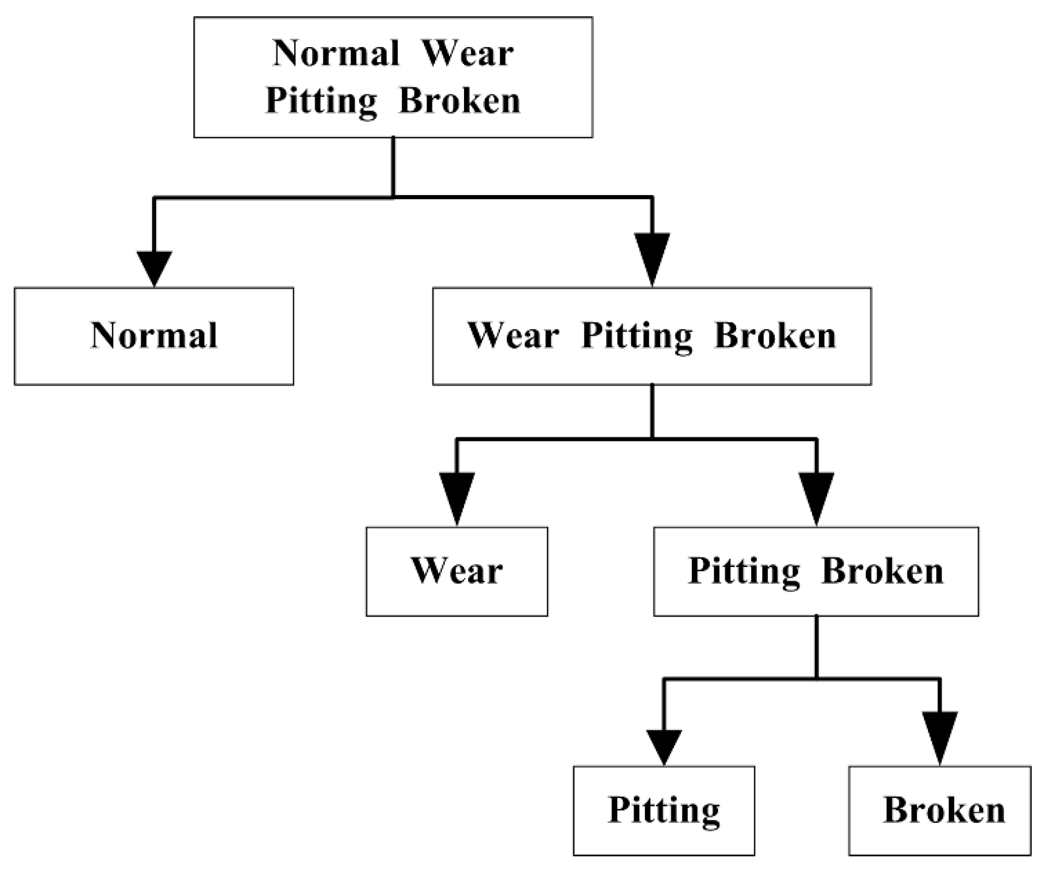
Figure 1. Four-class SVM recognition flow chart for gearbox fault diagnosis.
Machines 10 01186 g001
Figure 2. Connection chart of the gearbox experimental device based on the accelerometer.
Machines 10 01186 g002
Figure 3. Gearbox fault diagnosis experimental test platform.
Machines 10 01186 g003
Figure 4. Workflow chart of gearbox fault diagnosis based on the 1DCNN-IPSO-SVM model.
Machines 10 01186 g004
Figure 5. Framework of the gearbox fault diagnosis model based on multi-model feature fusion.
Machines 10 01186 g005
Figure 6. Parameter flow chart of the gearbox fault diagnosis based on parallel feature fusion.
Machines 10 01186 g006
Figure 7. Time−domain diagram of four types of the gearbox vibration data.
Machines 10 01186 g007
Figure 8. Frequency−domain diagram of four types of the gearbox vibration data.
Machines 10 01186 g008
Figure 9. IPSO-SVM fitness curves in the model optimization.
Machines 10 01186 g009
Figure 10. Average recognition accuracy by the proposed multi-model feature fusion model.
Machines 10 01186 g010
Figure 11. Confusion matrix of the fifth operation recognition result.
Machines 10 01186 g011
Table 1. Gearbox experimental data information.
TypeGearbox StatusData LengthMotor Speed
(rpm)
Sampling Frequency (kHz)Number of Data GroupsExpected
Output
1Normal1024900615000
2Wear1024900615001
3pitting1024900615002
4Broken1024900615003
Table 2. 1DCNN model parameters.
LayerKernel SizeStepOutput Size
Conv11 × 161 × 464 × 256
Max Pooling11 × 21 × 264 × 128
Conv21 × 81 × 264 × 64
Max Pooling21 × 21 × 264 × 32
Conv31 × 41 × 232 × 16
Max Pooling31 × 21 × 132 × 16
Conv41 × 21 × 116 × 16
Max Pooling41 × 21 × 116 × 16
FC11000 1000
FC210 10
Table 3. Calculation equations of the time–frequency index.
NumberIndicator NameEquationAnnotation
1Root mean square x r m s = 1 N i = 1 N x i 2 xi is the ith value of the signal x; N is the total number of data
2Kurtosis K a = i = 1 N [ x ( i ) x ¯ ] 4 ( N 1 ) σ 4 x ¯ is the signal mean; σ is the standard deviation
3Peak factor c = x p x r m s x p is the peak
4Impulse factor I = x p | x ¯ | | x ¯ | is the average of the absolute values
5Waveform factor W = x r m s x ¯ x r m s is the root mean square value
6Margin factor L = x p x r x r is the square root amplitude
7Barycenter frequency C = 0 + f P ( f ) d ( f ) 0 + P ( f ) d ( f ) P ( f ) is the power spectrum of the signal
8Root mean square frequency R M S = 0 + f 2 P ( f ) d ( f ) 0 + P ( f ) d ( f ) P ( f ) is the power spectrum of the signal
Table 4. Partial normalized eigenvalues.
StateNormal Wear Pitting Broken
Feature
Root mean square0.36790.2077 0.2196 0.4183
Kurtosis0.0657 0.30040.09050.3676
Peak factor0.1702 0.39680.23590.5132
Impulse factor0.1772 0.36880.21760.4937
Waveform factor0.3089 0.24580.18610.3442
Margin factor0.18610.35950.21380.4862
Barycenter frequency0.52610.54510.40540.5020
Root mean square frequency0.57500.57490.41880.5235
Complemented feature 1 and 20000
Table 5. Eigenvalues from 1DCNN.
StateNormalWearPittingBroken
Feature
f10.999970.000100.999990.99636
f20.000380.999920.989990.00005
f30.999980.999560.999970.00012
f40.000090.000440.000030.99981
f50.000390.999920.993410.00002
f60.999960.000220.999990.99947
f70.999400.000140.999990.00006
f80.002830.000400.984950.99878
f90.999870.999940.007950.99799
f100.001700.999960.000020.99997
Table 6. Eigenvalues from the parallel fusion method.
StateNormalWearPittingBroken
Feature
d11.002130.300401.065421.00046
d20.36790 1.02126 1.07473 0.21960
d31.014361.075441.123970.23590
d40.177200.368800.493701.02322
d50.308901.029691.051350.18610
d61.017130.359501.111921.02208
d71.129420.545101.118920.40540
d80.575010.574901.115431.08303
d90.999870.999940.007950.99799
d100.001700.999960.000020.99997
Table 7. Average accuracy and standard deviation of the four models.
Diagnosis MethodTime–Frequency Features + IPSO-SVM1DCNN-Softmax1DCNN-IPSO-SVMMulti-Feature
Fusion Model
Ten times average
classification accuracy/%
96.496.897.798.3
standard deviation0.41900.41470.35530.2108
Publisher’s Note: MDPI stays neutral with regard to jurisdictional claims in published maps and institutional affiliations.