A New Model for Remaining Useful Life Prediction Based on NICE and TCN-BiLSTM under Missing Data

Abstract

The Remaining Useful Life (RUL) prediction of engineering equipment is bound to face the situation of missing data. The existing methods of RUL prediction for such cases mainly take “data generation—RUL prediction” as the basic idea but are often limited to the generation of one-dimensional test data, resulting in the extraction of the prediction network. Therefore, this paper proposes a multivariate degradation device based on Nonlinear Independent Components Estimation (NICE) and the Temporal Convolutional Network–Bidirectional Long Short-term Memory (TCN-BiLSTM) network for the RUL prediction requirements in the case of missing data. First, based on the NICE network, realistic data are generated through reversible sampling; then, the filling of multivariate missing data is completed. Next, the filled multivariate degradation data are processed to generate multivariate degradation data and predicted labels for constructing the training set and test set. Based on this, a residual life prediction model integrating TCN and the BiLSTM network is proposed. To evaluate the proposed method, this paper takes an example of the RUL prediction of aeroengines to perform multivariate degradation data-filling and prediction tasks. The results demonstrate the superiority and potential application value of the method.

1. Introduction

The integrated application of multidisciplinary technical methods in cross-disciplinary fields provides a technical approach for the Prognostics and Health Management (PHM) of multiple and complex degraded equipment, which has gradually become a hot research topic in the fields affecting reliability workers and maintenance technicians [1,2,3,4,5,6,7,8,9,10]. Multi-degradation equipment integrating mechanical, electrical, hydraulic, and other technologies often has high reliability, a long life, and high value, and its performance degradation and fault status are closely related to multiple characteristic variables of the system. Therefore, identifying the underlying evolutionary mechanism from the above characteristic variables has gradually become the focus of attention in the fields of current equipment status assessment, fault diagnosis, and Remaining Useful Life (RUL) prediction [11,12,13,14,15,16,17].

For multi-degraded equipment, some data may be inevitably missing owing to machine failures (e.g., measurement sensor failures) or human factors (e.g., recording errors) in engineering practice. If such incomplete data are used to predict the RUL of equipment, it would be difficult to accurately describe the law of equipment degradation, which in turn affects health management and maintenance decisions concerning equipment. Therefore, generating or filling high-precision and high-reliability multidimensional data is of great significance for the prediction and health management of multi-degraded equipment [18,19].

2. Literature Review

The generation model of randomly generating samples by learning the probability density of observable data has received extensive attention in recent years. The deep generative model with multiple hidden layers in the network structure has become a research hotspot with better generation ability. The training of a deep generative model [20] is difficult and the model structure is complex, but in addition to being able to generate new samples, the generative model has also achieved great success in image reconstruction, missing data filling, density estimation, style transfer, and semi-supervised learning. The earliest deep generative models are variants based on Boltzmann machines. The most important derivative models are Restricted Boltzmann machines (RBM), which use the sampling method to approximate the likelihood function [21], Deep belief network (DBN) and Deep Boltzmann machines (DBM) based on RBM. Such models can learn high-dimensional features and high-order probability dependencies and are successfully applied in the fields of dimensionality reduction and feature extraction.

The depth generation method represented by the variational encoder is based on the autoencoder structure. The sample is mapped to the latent variable in the low-dimensional space through the encoding (Encoder) process, and then the latent variable is restored to the reconstructed sample through the decoding (Decoder) process. The Importance weighted autoencoders (IWAE) of the encoder in the variational lower bound is weakened [22], and the label information is integrated into the model. Conditional variational auto-encoder (CVAE) for supervised learning [23,24] and semi-supervised variational auto-encoder for semi-supervised learning [25,26]. The model that incorporates the convolutional layer into the VAE is called the Deep convolutional inverse graphics network (DC-IGN) [27]. Adversarial autoencoders (AAE) [28] with adversarial ideas. Ladder variational autoencoders (LVAE) with step structure [29]. In addition, Vector quantized variational auto-encoders (VQ-VAE) [30,31] is proposed by hiding the discretized variables.

The deep generation method represented by generative adversarial networks [32] optimizes the model parameters through the adversarial behavior between the generator and the discriminator to avoid solving the likelihood function. Deep convolutional generative adversarial networks (DCGAN) [33] is the first important improvement to GAN. It screens out the best set of generators and discriminators in a variety of structures, which significantly improves the stability of GAN training. WGAN [34] (Wasserstein GAN) proposed replacing KL divergence and JS divergence with Wasserstein distance to solve the problem of instability of GAN and basically eliminate the model collapse problem on simple datasets. In the field of image generation, BigGAN [35] successfully applied it by introducing a residual structure. In addition, by inputting label information as additional information into the generator, Condition GAN (CGAN) [36] combines samples with label information. However, most adversarial networks face problems such as unstable training.

Although VAE replaces the real data by solving the variational lower bound of the likelihood function, the resulting approximation model does not produce the best results. Although GAN avoids optimizing the likelihood function and retains the accuracy of the model by using the method of model confrontation and alternating training, there are various problems in the training process. Therefore, it is important to study a deep generation model that can ensure the accuracy of the model and is easy to train. The flow model with the advantages of accurate log-likelihood assessment and accurate latent variable inference [37,38] is still in its infancy. Since OpenAI’s Glow [39] based on the flow model proposed by NeurIPS in 2018 has been successfully applied to image generation tasks many times, researchers have once again focused on the flow generation model. Among them, Non-linear Independent Component Estimation (NICE), as the first variant based on a flow model, is favored by scholars for its powerful data generation ability. GE et al. [40] proposed a generation network based on the NICE framework to simulate the one-dimensional daily load curve of a distribution network, the study shows that the model can better capture the temporal and spatial correlation of a daily load curve. Xue Yang et al. [41] proposed a generation network based on the NICE framework to enhance the distributed photovoltaic stealing data curve. By comparing the generation effect of GAN and VAE, NICE has more accurate likelihood estimation and the generated samples are closer to the real data curve. However, the re-search on multidimensional data generation only stays in the field of image processing and has not been applied to the generation of multidimensional time series data.

As the core of PHM technology, the data-driven residual life prediction method has received extensive attention from academia and industry and achieved rich results due to the advantages of no need to determine the degradation model in advance, low requirements for professional mechanism knowledge, wide application range, and low prediction cost. The machine learning-based method uses classical network models (such as support vector machines, auto encoders, convolutional neural networks, etc.) to deeply mine the potential information and rules contained in complex data, self-learn the mapping relationship between equipment performance degradation law or monitoring data and failure time, and obtain equipment failure time by rolling extrapolation or direct prediction. In the field of residual life prediction of multivariate degradation equipment, many scholars related to deep learning and neural networks have conducted multivariate time prediction research. It mainly includes RNN-based structures and CNN-based structures.

As a deep recurrent structure, the RNN network regards the RUL estimation problem as a time series regression problem, which is very suitable for processing time series data and using deep learning models to solve it. Gugulothu [42] applied the RNN network to time series prediction, which does not depend on any degradation trend hypothesis, is robust to noise, and can handle missing values. Zheng [43] applied the LSTM network to RUL estimation. Compared with RNN, LSTM controls information flow by introducing three gate structures: input gate, forgetting gate, and output gate, which solves the problem of long-term dependence of RNN. In addition, Bi-RNN [44] refers to the combination of two independent one-way RNNs, and Bi-LSTM [45] refers to the combination of two independent one-way LSTMs, which exploits more information.

In recent years, the CNN network has been mainly used for tasks such as feature extraction and image classification. The authors of [46] first attempted to use the CNN structure for RUL estimation and prediction. Unlike the CNN structure in image processing, the convolution and pooling operations in the prediction model are applied along the time series, and through the deep architecture, the learned features are high-level abstract representations of the original signal. The authors of [47,48] state that based on the CNN structure, the time series structure TCN with causal dilation convolution is adopted, and the extracted features are used as the input of the time series structure. The prediction results depend on the depth of the network and the size of the dilation factor.

The variant networks based on RNN [42] structure include LSTM [28], BiRNN [44], and Bi-LSTM [13,45]. The variant networks based on the CNN structure are mainly DCNN [46] and TCN [47,48]. Wang J et al. [13] proposed a new data-driven method using the BiLSTM network for RUL estimation, which can make full use of the bidirectional sensor data sequence. Zhang H et al. [18] proposed a deep learning model based on TCN and Attention for real-time motor fault diagnosis. Zhao C. et al. [45] proposed a two-channel hybrid prediction model based on CNN and the BiLSTM network. Considering that the multivariate degradation equipment contains multiple dimensions of degradation information, the degradation laws are different, the life contribution rates corresponding to different dimensions are different, and the coupling relationship between each dimension is complex. The above model in the prediction process of only a single network is bound to have limitations. Specifically, although the TCN network can perform convolution operations in parallel and perform local feature extraction quickly on the basis of CNN, the prediction result (i.e., the remaining life at the current time) is only related to the previous time. As a typical representative of RNN, BiLSTM can effectively avoid the drawbacks of TCN network, but its short-term memory is not as accurate and fast as convolution operation. Therefore, in order to obtain more accurate residual life prediction results, it is an urgent requirement to fuse TCN.

In order to solve the abovementioned practical problems in data generation and RUL prediction, this paper proposes a prediction model based on NICE and TCN-BiLSTM under-missing data. Specifically, the method mainly consists of a two-level architecture. The first-level architecture uses a deep neural network based on the NICE model to model the distribution of multisource degraded data so that multidimensional degraded data can be reconstructed. In the second-level architecture, this paper combines the advantages of TCN parallel computing and BiLSTM long-term memory and proposes a TCN-BiLSTM model to predict the RUL of equipment. Among them, TCN mainly undertakes feature extraction and captures short-term local dependencies, while BiLSTM mainly undertakes long-term memory and captures long-term macro dependencies. A RUL prediction is performed on the filled multidimensional degraded data by the TCN-BiLSTM model. The contributions of this paper are twofold:

(1)

This paper introduces NICE technology, which can fully mine the true distribution laws behind missing data, map training data to a standard normal distribution, generate realistic data through reversible sampling, and then fill in missing values. Thus, multivariate degradation data can be generated in the full-time sense;

(2)

Compared with the literature [13,48], the method proposed in this paper can capture both long- and short-term dependencies, effectively ensuring that the extracted features fully reflect the health status of the device.

The remaining sections are arranged as follows. Section 3 describes the problem formulation. Section 4 introduces the multivariate degradation data filling model based on the NICE model and the multivariate degradation data forecasting model based on the TCN-NICE model. Section 5 is the example validation part, choosing multivariate degradation dataset C-MAPSS as the validation dataset. Section 5.1 describes the implementation of this experiment. Section 5.2 carries out the dataset and processing work. Section 5.3 applies the NICE model to the multivariate degradation data filling task. Section 5.4 applies the TCN-BiLSTM model to the multivariate degradation data filling task. Section 6 is the conclusion, which summarizes the innovative points of this paper.

3. Problem Formulation

For random degradation devices monitored by missing multisource sensors (i.e., there are missing multivariate degradation data), assuming that there are $N$ devices of the same model in total, $x_i^j(t)$ is marked as the $j(1\le i\le N)$ sensor of the $i(1\le i\le N)$ device at $t(t>0)$. For monitoring data, the corresponding monitoring time is marked as $t_i^j=[t_i^{j,0},t_i^{j,1},\cdots ,t_i^{j,K_{ij}}]$, where $K_i^j$ is the total number of monitoring samples of the $i$ device and the $j$ sensor. Assuming that the sampling numbers of the $S$ groups of sensors of the same device are the same, the monitoring dataset taken by the $i$ sensor of the $j$ device can be recorded as $x_i^j=[x_i^{j,0},x_i^{j,1},\dots ,x_i^{j,K_{ij}}]$, and the multisource sensor monitoring data of the $i$ device can be recorded as:

$$X_i=\left[\begin{array}{c}{x}_i^1\\ x_j^2\\ ⋮\\ x_j^S\end{array}\right]=\left[\begin{array}{cccc}{x}_i^{1,0}& x_i^{1,1}& \cdots & x_i^{1,K_{i,j}}\\ x_i^{2,0}& x_i^{2,1}& \cdots & x_i^{1,K_{i,j}}\\ ⋮& ⋮& \ddots & ⋮\\ x_j^{S,0}& x_i^{S,1}& \cdots & x_i^{S,K_{i,j}}\end{array}\right]$$

(1)

where $x_i^{j,k}=x_i^j(t_i^{j,k})(k=0,1,\cdots ,K_{i,j})$ represents the monitoring data of the $j$ sensor of the $i$ device at the time $t_i^{j,k}(k=0,1,\cdots ,K_{i,j})$.

The filling of missing multidimensional degenerate data is essentially a problem of learning the degenerate distribution of multidimensional data. Among them, considering the complexity and coupling of the monitoring data of multivariate degradation equipment, the data missing mode is Missing Completely At Random (MCAR), which means that the missing data of each dimension have nothing to do with the dimension or any other variable. The missing rate for each dimension is the same. If the data are missing, $x_i^{j,k}=NAN$. Send $X_i$ into the deep generative network model, expecting enough real generated data to be recorded as ${\tilde{X}}_i$ in order to fill in the missing values.

Prediction of populated multidimensional degraded data is essentially a problem of learning the degradation trend of multidimensional data. Assuming the monitoring sampling interval is the same, each sampling is recorded as a unit of time, and when the equipment fails, the length of all monitoring moments ($t_i^j$) is recorded as the life $L=K_i^j$; therefore, the RUL of each sampling is $RUL=L-k(k=0,1,\cdots ,K_{i,j})$. Specifically, in the deep learning prediction framework, the input training data are multivariate degradation data, and the neural network model maps the degradation trend to the RUL; that is, the predicted label is the RUL. Some degradation data are input in the verification set, and the output corresponds to RUL.

Based on the above analysis, this paper focuses on the following questions:

(1)

How to design a data generation model to achieve optimal filling of missing parts of the data;

(2)

How to build the RUL prediction network model to achieve accurate prediction of the RUL of the equipment.

4. Multidimensional Missing Data Generation and Prediction

4.1. Multivariate Degraded Data-Filling Model Based on the NICE Model

The main purpose of this section is to introduce the core idea of the flow model through theoretical analysis, as well as how it, as a deep generative model, trains DNNs and infers new data representations from prior distributions to generate new samples.

The basic idea of the flow model is that a complex data distribution must be mapped to a simple data distribution via a series of transformation functions. If these transformation functions are reversible and easy to obtain, the simple distribution and the inverse function of the reversible transformation function constitute a deep generative model. As shown in Figure 1.

Specifically, the flow model assumes that the original data distribution is $P_X(x)$, the prior hidden variable distribution is $P_Z(z)$ (usually a standard Gaussian distribution), the reversible transformation function is $f(x)$ ($z=f(x)$), and the generating transformation function is $g(x)$ ($g(x)=f^{-1}(x)$). The variable substitution method based on the probability distribution density function can be obtained as:

$$\begin{array}{l}{P}_X(x)=P_Z\left(f\right(x))\left|\det \frac{\partial f(x)}{\partial x}\right|\\ =\frac{1}{{(2\pi )}^{D/2}}\exp (-\frac{1}{2}{‖f(x)‖}^2)\left|\det \frac{\partial f(x)}{\partial x}\right|\end{array}$$

(2)

where, $D$ is the dimension of the original data, $\left|\det \frac{\partial f(x)}{\partial x}\right|$ is the reversible transformation function $f(x)$, and the Jacobian determinant is $x$. Higher-dimensional monitoring data increases the computational complexity of the Jacobian determinant, resulting in model fitting. The burden of the flow model is more than the process of solving the inverse function of the invertible function. Therefore, the flow model needs to ensure that its Jacobian determinant is easy to calculate in addition to the conversion function $f(x)$:

$$\begin{array}{l}\log \left(P_X\right(x))\\ =\log \left(P_Z\right(f(x)))+\log (\left|\det \frac{\partial f(x)}{\partial x}\right|)\\ =-\frac{D}{2}\log (2\pi )-\frac{1}{2}{‖f(x)‖}^2+\log \left|\det \frac{\partial f(x)}{\partial x}\right|\end{array}$$

(3)

The NICE model is a DNN based on the flow model framework, which mainly includes basic structures such as an additive coupling layer, dimensional blending, and a scale layer. Similar to the variational auto encoder, the training process of the NICE model can be divided into an encoding phase and a decoding phase. In the encoding stage, NICE maps the input samples to a Gaussian distribution using a series of reversible transformations such as the additive coupling layer, dimension mixing, and scale transformation layer. In the decoding stage, the inverse process of the encoding stage is established, and the weights in the encoding stage are directly used, resampling from the normal distribution to obtain the generated data. Among them, the encoding stage determines the quality of the generated model, which is theoretically error-free. Note that the loss function of the NICE model is the inverse of the model optimization objective:

$$\begin{array}{l}{\mathrm{loss}}_{\mathrm{NICE}}=-\log \left(P_X\right(x))\\ =\frac{D}{2}\log (2\pi )+\frac{1}{2}{‖f(x)‖}^2-\log \left|\det \frac{\partial f(x)}{\partial x}\right|\end{array}$$

(4)

Specifically, the structure of the NICE model is shown in Figure 2. First, input $X_i$ is randomly divided into two parts ($X_{i,1}^{(0)}$ and $X_{i,2}^{(0)}$) according to the dimension, and enters the first additive coupling layer, where $X_{i,1}^{(0)}$ directly obtains $h_1^{(1)}$, $X_{i,1}^{(0)}$. After the coupling of $m_1$, add it to $X_{i,2}^{(0)}$ to obtain $h_2^{(1)}$; that is, the additive coupling layer does not perform the coupling operation on the first part. Then, swap $h_1^{(1)}$ and $h_2^{(1)}$, and then enter the next additive coupling layer, where $h_2^{(1)}$ directly obtains $h_2^{(2)}$, and $h_2^{(1)}$ is coupled with $m_2$ and then added with $h_1^{(1)}$ to obtain $h_1^{(2)}$, and so on, with four additive coupling layers. Take the coupling layer structure as an example. Finally, $h_1^{(4)}$ and $h_2^{(4)}$ are jointly inputted into the scale compression layer (S) and $z_{i,1}$ and $z_{i,2}$ are output and concatenated into z_i.

Training with the NICE model. Send X_i into the NICE model for coding and then sample the standard normal distribution to obtain enough real generated data ($X_i^{\prime }$) to fill in the corresponding missing values and record the filled data as ${\tilde{X}}_i$.

4.2. Multivariate Degraded Data Prediction Model Based on the TCN-BiLSTM Model

The main purpose of this section is to introduce the core idea of the TCN-BiLSTM model through theoretical analysis, how it is used as a prediction model to extract features from multidimensional data, and how to map training features to RUL in order to achieve RUL prediction.

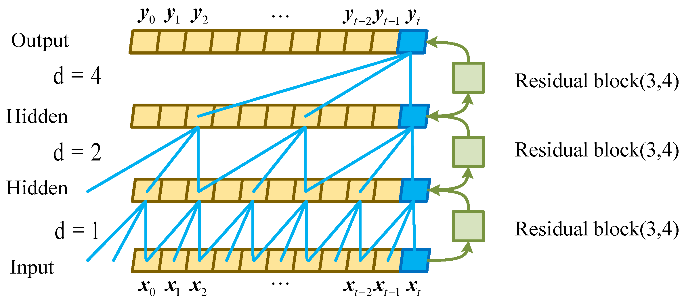
The TCN network proposed by Bai et al. [47] is a CNN model with a special structure. It is based on the traditional one-dimensional CNN called 1-D FCN, combined with causal convolutions and dilated causal convolutions. A new network model is obtained by combining dilated causal convolutions and residual blocks in the TCN architecture. In order to input the time step as in RNN, the output time step is also the same length; that is, the input of each time has a corresponding output, which uses the structure of 1-D FCN in each hidden layer. The time length of the input and output are the same, and the same time step is maintained; in order to ensure no leakage of historical data, we do not use a traditional convolution but a causal convolution is selected. The data output at time $y_t$ is only related to the data at time $t$ and before time $t$, that is $x_0-x_{t-1}$. In order to effectively deal with the problem of long historical information, dilation causal convolution is introduced, which still has causality, and the dilation factor is introduced, which is generally dilated. The coefficient is an exponential power of 2. In order to solve the problem of gradient disappearance that may be caused by a deeper network structure, a residual block is introduced to improve the generalization ability of the TCN structure. As shown in Figure 3, a TCN structure with a convolution kernel size and a maximum expansion factor of three and four is simulated.

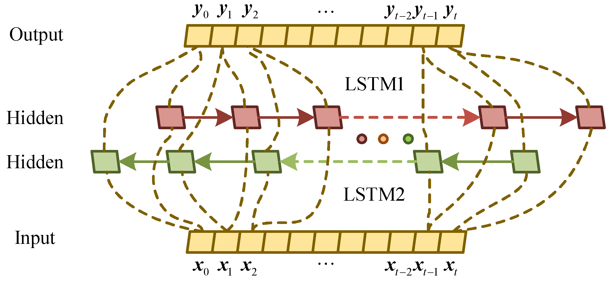
The Bi-LSTM neural network structure model is divided into two independent LSTM hidden layers. As shown in Figure 4, the input sequence is input to the two LSTM neural networks in positive and reverse order for feature extraction. The vector formed after splicing is used as the final feature expression. The key to Bi-LSTM is that the feature data obtained at time $t$ holds both past and future information. Experiments have shown that this neural network structure model is better than a single LSTM structure model for text feature extraction efficiency and performance. Furthermore, the two LSTM neural network parameters in Bi-LSTM are independent of each other; they only share a list of multivariate degradation data vectors.

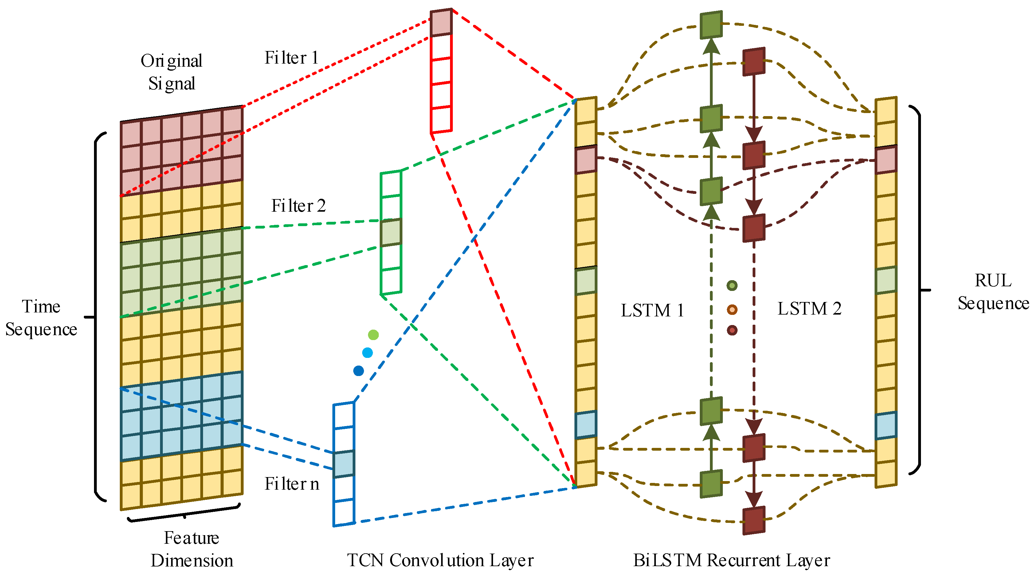
In order to fuse the advantages of TCN parallel computing and BiLSTM long-term memory, the structure of the TCN-BiLSTM model is shown in Figure 5. Specifically, first, the ${\tilde{X}}_i$ obtained in Section 3 is processed by a sliding time window with a window length of $N\times S$, and multiple matrices with a dimension of $rul=L-k(k=[0,1,\cdots ,K_{i,j}])$ and their corresponding RUL sequences *3 are combined to form the $TimeSequence$ and $RULSequence$ data pair. The processed data pairs are used as training data and sent to the TCN-BiLSTM network model. Subsequently, through $n$ dilated causal convolutions and residual operations, we extract the local features of multivariate degraded data in parallel, input the extracted feature sequence into the BiLSTM network, mine deep sequence information through forward LSTM and reverse LSTM, and finally obtain the accurate RUL.

5. Experimental Research

As the “crown jewel” of modern manufacturing and the “heart” of aircraft, the aeroengine is the key piece of equipment that provides flight power for aircraft. The abnormality of the system causes the engine thrust to drop, which can lead to serious accidents such as in-flight parking, directly reducing the flight safety and mission reliability level. At present, the performance monitoring and health status assessment of aeroengines face the problems of unbalanced fault data, high test costs, and a lack of real data on individual equipment. This paper takes aeroengines as an example to perform multivariate degradation data-filling and prediction tasks to verify the effectiveness of the proposed method.

5.1. Implementation

In order to test and validate the potential contribution of the proposed approach for future real-world applications, this method has been implemented into a prototype software system using Python 3.6.13. In particular, the NICE and TCN-BiLSTM models are implemented using Keras 2.3.1, a Python library for developing and evaluating deep learning models. The resources used in order to integrate the aforementioned system were a computer with an Intel i7 processor (Intel(R) Core(TM) i7-10770K CPU @ 3.80 GHz, regarding the processing power, and an 128 gigabyte RAM memory. The operating system that the proposed system was hosted and tested on was Microsoft Windows 10.

5.2. Data Set Introduction and Preprocessing

This section selects the C-MAPSS aeroengine simulation experimental dataset [49] released by NASA to verify the method. The dataset consists of multiple multivariate time series, including three operating settings and 21 types of sensors that have a significant impact on engine performance, for a total of 26-dimensional data. A total of four types of datasets are recorded under different working states and failure mode combinations as the scale of failures continues to expand. Each dataset is further divided into training and testing subsets. In the training set, the entire time series of each engine from normal operation until system failure is recorded. In the test set, the time series for each engine ends some time before the system fails. The specific information is shown in

Table 1. C-MAPSS dataset.

No.	Train Engines	Test Engines	Conditions	Fault Modes
FD001	100	100	1	1
FD002	260	260	6	1
FD003	100	100	1	2
FD004	249	249	6	2

.

This paper uses the data of the No. 1 engine in the training set FD001 dataset to generate multisource degradation data, where sensors1–21 represent the relevant feature quantities in the dataset. Considering that the engine performance degradation is continuous, its characteristic quantities should also show a certain trend change in the time series. First, we draw a time series diagram for all sensor data, as shown in Figure 6.

As can be seen from Figure 6, sensor1, sensor5, sensor6, sensor10, sensor16, sensor18, sensor19, and other feature quantities are not sensitive to time series signals or are discrete variables, and they play a small role in feature engineering such as the construction of comprehensive health indicators. Therefore, the data generation of these sensors is of little significance, and these sensors are screened, and finally, the remaining 14-dimensional data (sensor2, sensor3, sensor4, sensor7, sensor8, sensor9, sensor11, sensor12, sensor13, sensor14, sensor15, and sensor17) with large changes are selected.

In order to efficiently train and mine deep-level features of the deep learning model in the later stage, we must perform the necessary preprocessing operations on the original data for training. First, the complete dataset of the 14-dimensional degradation monitoring are processed according to the MCAR missing mechanism in Section 2. Further, each dimension of each sample of the missing data is linearly normalized to the (−1,1) interval to obtain the training sample of the NICE model. The normalization formula is as follows:

$$X_{new}=2\times (\frac{X_i-X_{\min }}{X_{\max }-X_{\min }})-1$$

(5)

where $X_{\max }$ and $X_{\min }$ are the extreme maximum and minimum values of a certain dimension sample, respectively, and $i$ is the current dimension.

5.3. Multivariate Degraded Data-Filling

The engine dataset uses the sensor data measurement period as the engine life metric. When the measurement period reaches the maximum, the engine has been shut down, and each row of the corresponding data indicates a new time step in the measurement time series by default. The normalized data are input into the NICE model for data generation. Some parameters of the NICE model are set out as shown in

Table 2. NICE model parameters.

Mode	Additive Coupling Layers	Coupling Layers	Neurons in Each Layer	Batch Size	Iterations
NICE	8	5	1000	64	1000

.

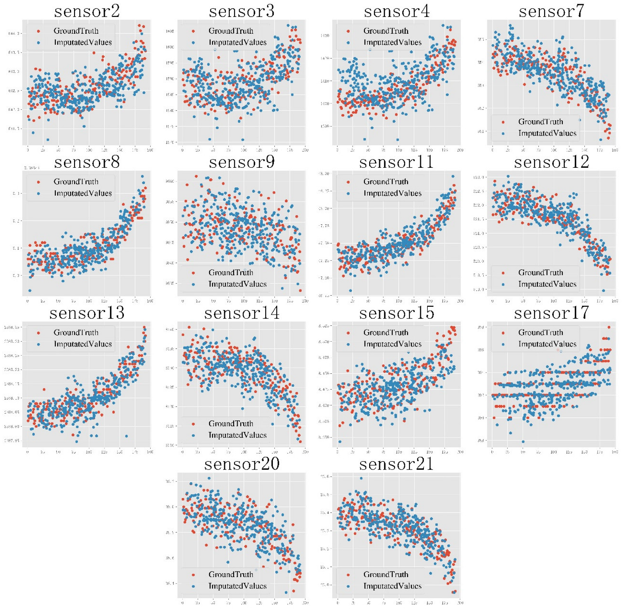
According to the parameter configuration in Table 2, the multisource degradation data generated by training the NICE model is shown in Figure 3.

Figure 7 shows the generation diagram of the degradation data of each sensor in the absence of different dimensions. It is clear that no matter whether the degradation trend is increasing or decreasing, the data generated by the NICE model can well cover the degradation of multiple sensors of the aeroengine. The trend is closer to the distribution characteristics of the real degradation data.

Furthermore, in order to quantify the generation effect, we use the two-way Hausdorff distance [50] to quantify the distribution error between the generated samples and the training samples of different sensors. The calculation formula is as follows:

$$\begin{array}{l}H(A,B)=max[h(A,B),h(B,A)]\\ h(A,B)=\underset{a\in A}{\max }\underset{b\in B}{\min }‖a-b‖\\ h(B,A)=\underset{a\in B}{\max }\underset{b\in A}{\min }‖b-a‖\end{array}$$

(6)

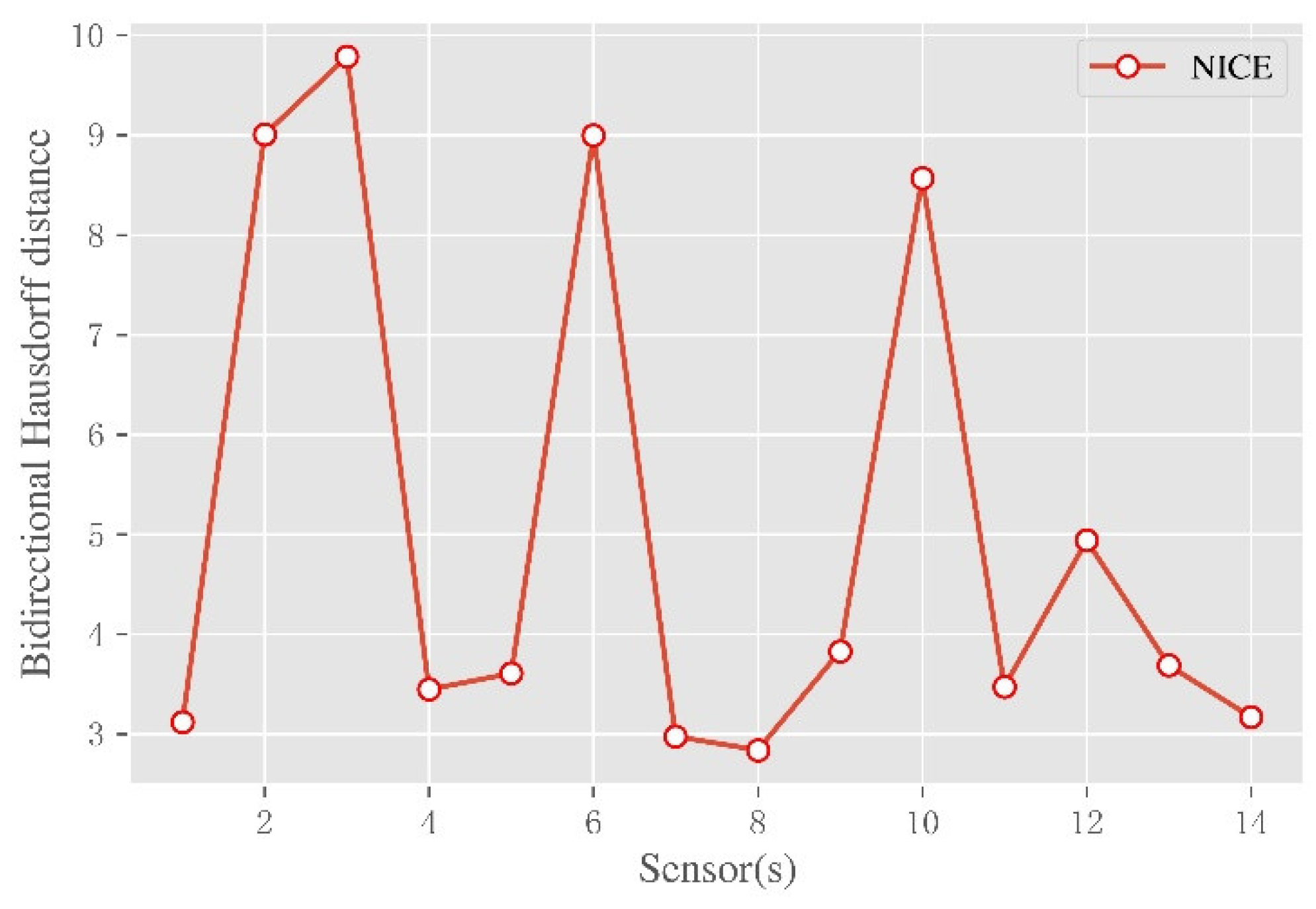
Among them, $H(A,B)$ is called the two-way Hausdorff distance, $h(A,B)$ is called the one-way Hausdorff distance from point set A to point set B, and $h(B,A)$ is called the one-way Hausdorff distance from point set B to point set A. A plot of the distances of the NICE model in different dimensions is shown in Figure 8.

As can be seen from Figure 8, after the missing data are sent to the NICE network and trained, the accuracy of the generated model is measured by the bidirectional Hausdorff distance. Among them, the sensor8 sensor has the highest accuracy and is numerically equal to 2.83, and the sensor4 sensor has lower accuracy and is numerically equal to 9.78. It shows that under different dimension sensors, the bi-directional Hausdorff distance obtained by the proposed method is low and close to the original distribution.

5.4. Multivariate Degraded Data RUL Prediction

5.4.1. Multidimensional Sliding Time Window

In this section, the prediction ability of the TCN-BiLSTM model is verified. A detailed description of the FD001 data set is shown in

Table 3. FD001 dataset.

FD001	Training Set	Testing Set
Number of engine units	100	100
Number of data	26,631	13,096
Minimum running cycle	128	31
Maximum running cycle	362	303
Mean running cycle	206.31	130.96
Number of time windows	30	30
Samples of sliding time windows	17,731	100

, including the mechanism and average of training set and test run cycles, respectively. Because the engine with the smallest running cycle appears in the test set, its running cycle is 31, and the time window size cannot be uniformly set to a value greater than 31. Otherwise, part of the test data cannot be processed, thus generating a prediction result. At the same time, a smaller time window is not suitable because it adversely affects the prediction accuracy. The authors of [51] set all time window sizes to 30. Specifically, as each cycle contains 14-dimensional data, when the prediction step size is 1, the maximum sliding time window can be set to 30.

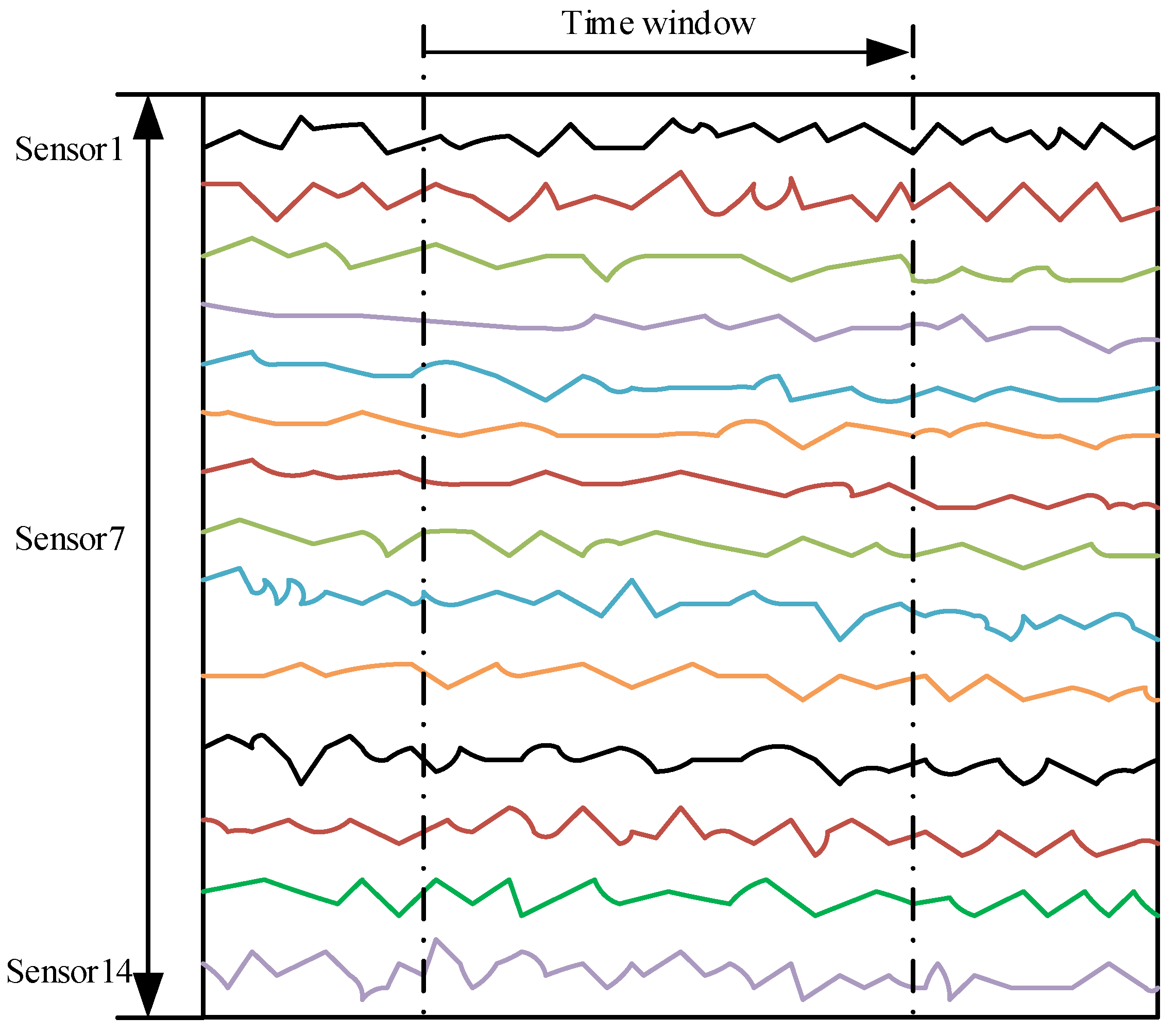
According to the settings in Table 3, the training set and the test set are divided. The training dataset is the failure degradation data of 100 engines of the same model throughout the life cycle and their corresponding true RUL labels. The test dataset is the degradation data of another 100 engines of the same model after stopping at a certain time and their corresponding real RUL labels. The input data in the training dataset is composed of 100 engines of the same model, including 14 sensors, which are processed by sliding time windows. The RUL times corresponding to each cycle are processed by sliding time windows, and the tensor dimension (batch_size, output_dim) is (17,731, 1). As shown in Figure 9, the input data in the test data et are composed of 14 sensors of the same model and another 100 engines processed by sliding time windows, and its tensor dimension (batch_size, timesteps, input_dim) is (100, 30, 14). The output data are composed of the RUL corresponding to each cycle of the respective engine through sliding time window processing, and its tensor dimension (batch_size, output_dim) is (100, 1).

5.4.2. Predictive Model Configuration and Evaluation Metrics

We then build the TCN-BiLSTM model, which mainly includes the structure and hyperparameters of the model:

First, the number of filters used in the convolutional layers of TCN, nb_filters, is an important parameter that correlates with the predictive ability of the model and affects the size of the network. The experimental setting in this paper is 30;

Second, the size of the TCN receptive field is jointly determined by the kernel size (kernel_size) used in each convolutional layer, the stack number (nb_stacks) of the residual block, and the dilation list dilations of the dilated convolution. Here, kernel_size controls the spatial area/volume considered in the convolution operation. A good value is usually between 2 and 8. If the sequence depends heavily on $t-1$ and $t-2$, but less on the rest, choose a kernel size of 2/3. In NLP tasks, the larger the kernel size, the more significant the effect, but the larger the kernel size, the larger a network is produced. Moreover, nb_stacks indicates the number of stacks of residual blocks that need to be used, which is useful unless the sequence is long (i.e., it is only used when the training data are on the order of hundreds of thousands of time steps). Dilations are lists of dilations, such as [1(0), 2(1), 4(2), 8(3), and 16(4)]. They are used to control the depth of the TCN layer. In general, we consider a list with multiples of 2. One can guess how many dilations are needed by matching the receptive field (of the TCN) to the length of the features in the sequence. For example, if the input sequence is periodic, multiples of that time period may be required as inflation. In general, the input sequence must satisfy the following two conditions numerically: the sum of the integer power of 2 must not be less than the number of sliding time windows, 30. So setting it to 32 is acceptable. Moreover, although the size of the receptive field is numerically equal to the product of their three terms, the experimental results are not the same owing to the different combination methods, and the most effective combination method requires multiple experiments to be performed in order to determine this. According to the above rules, assuming that the receptive field is 32, the combinations that can be selected are 2-1-16, 4-1-8, and 8-1-4. Additionally, the activation function is set to “relu.”;

Thirdly, BiLSTM mainly includes the number of BiLSTM layers and the number of LSTM units contained in each layer of BiLSTM. The experiments in this paper set these two values to 32 and 128, respectively;

Finally, two fully connected layers are added to transition the output results, where the number of filters in the first fully connected layer is defined as 30, and its activation function is “relu.” The number of filters in the second fully connected layer is set to 1, and its activation function is “linear.”

In addition, in order to solve the problem of overfitting, the Dropout operation, the EarlyStopping operation, and the piecewise learning rate, LearningRateScheduler operation, are added. The training parameters include the number of iterations (epoch) and the number of batches (batch size), which are set to 250 and 512, respectively.

In order to quantitatively evaluate the prediction effect, this paper selects two evaluation indicators, the Root Mean Square Error (RMSE) and the Score function (Score), which are defined as follows:

$$\begin{array}{l}RMSE=\sqrt{\frac{1}{n}{\displaystyle \sum _{i=1}^n{\left(\overline{RU{L}_i}-RU{L}_i\right)}^2}}\\ \mathrm{Score}=\left\{\begin{array}{l}{\displaystyle \sum _{i=1}^n{e}^{-\left(\frac{\overline{RU{L}_i}-RU{L}_i}{13}\right)}}-1,\overline{RU{L}_i}-RU{L}_i<0\hfill \\ {\displaystyle \sum _{i=1}^n{e}^{\left(\frac{\overline{RU{L}_i}-RU{L}_i}{10}\right)}}-1,\overline{RU{L}_i}-RU{L}_i\ge 0\hfill \end{array}\right.\end{array}$$

(7)

Among them, $\overline{RU{L}_i}$ indicates the real RUL at the second moment, $RU{L}_i$ indicates the predicted RUL at the second moment, $n$ is the total number of predicted samples, and the penalty designed by Score is as follows. When the predicted $RU{L}_i$ is greater than the actual $\overline{RU{L}_i}$, the higher the function score, the worse the prediction result. From a practical point of view, if $RU{L}_i$ lags behind $\overline{RU{L}_i}$, the time to take corresponding measures also lags, which has serious consequences. Thus, higher penalties are given.

5.4.3. Experimental Results and Performance Analysis

The RUL prediction results for the last recorded data point for the test engine unit in FD001 are shown in Figure 10. Among them, the performance monitoring variables of the engine all change little in the initial stage of degradation, so the extracted features also change slowly in the early stage of degradation. In order to improve the accuracy of the model prediction, we assume that the equipment has no degradation in the early stage of operation, the equipment RUL label is set to piecewise linear, and the maximum value is set to the average life of the engine, 125. Test engine units are sorted by labels from largest to smallest for better viewing and analysis. It can be seen that the RUL value predicted by this method is close to the actual value. Especially in regions with small RUL values, the prognostic accuracy tends to be higher. This is because when the engine unit is operating close to failure, the fault signature is enhanced and can be captured for better prediction.

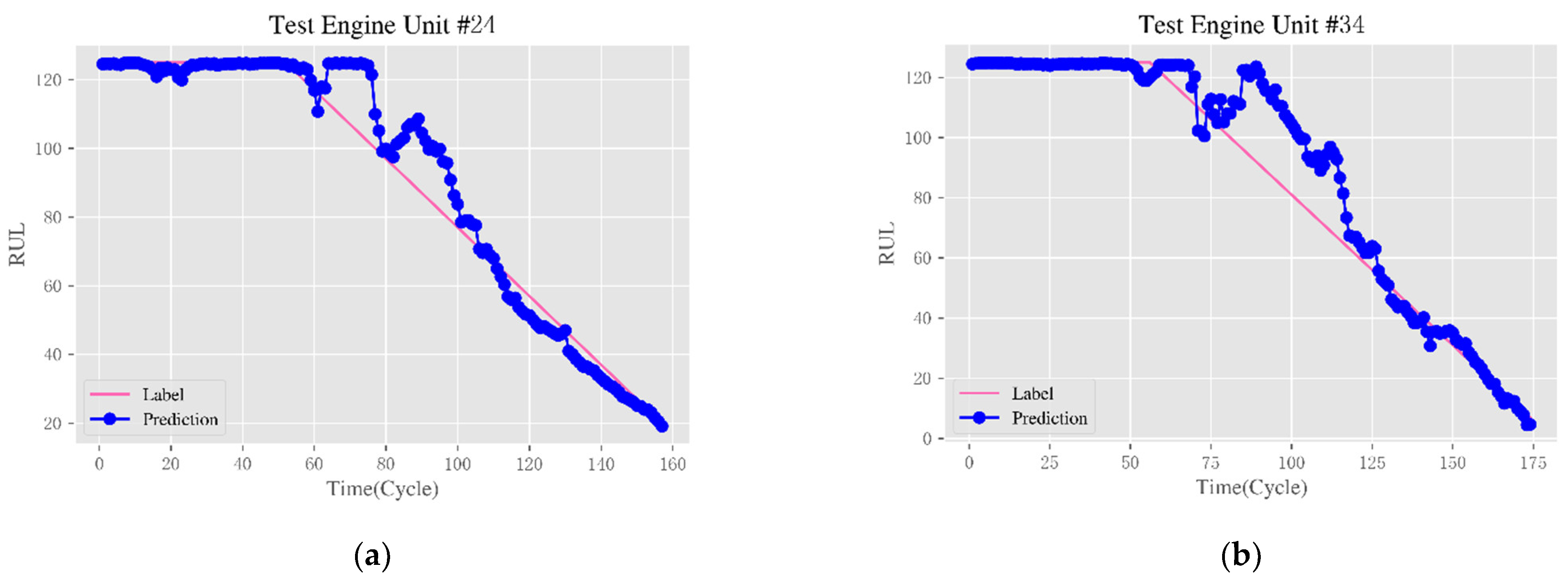
To further observe the prediction results of the method proposed in this paper, Figure 11 shows the full test cycle RUL prediction results of some test engines. Because the performance degradation state of the engine is related to the real-time and effective monitoring data, the more complete the monitoring data, the better the prediction effect. However, in the test dataset, the last part of the sensor measurements is not provided to examine the prognostic performance. Therefore, four engine instances with more test cycles are selected here; the 24th, 34th, 76th, and 81st, and the RUL prediction results of one full test cycle are given.

In addition, in order to study the influence of the combination of TCN receptive fields, Figure 12 shows the prediction results of three different combinations of TCN receptive fields and BiLSTM independently. Through comparison, it is found that under the four methods, especially in the area with a large RUL value, the effect of the TCN-BiLSTM layer is not as good. The combination of 2-1-16 and 8-1-4 predicts better results. In summary, the combination of 2-1-16 is selected.

Table 4. RUL prediction results of 100 engines under different combinations.

Mode	TCN (kernel_size-nb_stacks-dilations)			BiLSTM	TCN-BiLSTM
	2-1-16	4-1-8	8-1-4	32-128	2-1-16-32-128
RMSE	11.47	12.35	13.58	11.89	4.13
Score	206.26	230.30	328.42	294.29	74.26

presents the numerical results of these experiments.

5.4.4. Comparative Analysis of RUL Prediction Methods

In order to reflect the superiority of the method proposed in this paper, DCNN [51], MDBNE [52], LSTM [53], and other methods from the literature are introduced for comparison.

Table 5. Model RMSE and score results of the proposed method and related approaches.

Model	RMSE	Score
DCNN [51]	13.32	N/A
MDBNE [52]	17.96	640.27
LSTM [53]	12.81	N/A
TCN	11.47	206.26
BiLSTM	11.89	294.29
TCN-BiLSTM	4.13	74.26

shows the comparison of the prediction results between TCN-BiLSTM and existing prediction methods.

The experimental results in Table 5 show that the proposed TCN-BiLSTM structure is very suitable for multidimensional degradation data prediction. The TCN network is the first structure to use multidimensional feature extraction, which can quickly extract local features in parallel. The BiLSTM network is the second structure using circular information flow, and the integrated BiLSTM layer helps to improve the learning ability of the network. Because the proposed model is a combined model, the training time is longer than most shallow networks in the literature, so there is a problem of slow training speed. However, in terms of prediction accuracy and reliability, the proposed combined model further confirms the superiority of using parallel structure to extract original degradation features and cyclic structure to mine sequence hidden features.

6. Conclusions

Aiming at the problems of low generated sample accuracy and low residual life prediction accuracy in the case of multi-degraded equipment missing data, this paper proposes a data generation method based on the NICE model, which can achieve better generation results. The multivariate degradation data of the engine are verified. The main contributions of the work are as follows:

(1)

A multisource degradation data generation method based on the NICE model is proposed, which can quickly and accurately learn the real distribution behind multisource data;

(2)

A method for predicting the RUL of multidimensional degraded equipment based on the fusion of the TCN and BiLSTM models is proposed. First, multidimensional local features are extracted, and then depth information is predicted. Especially in the later stage, when the multi-degraded equipment is close to failure, the error between the predicted RUL value and the actual value is smaller;

(3)

Compared with other models, TCN-BiLSTM achieves superior performance. The effects of different receptive field combinations on the prediction performance are studied.

In future research, we will further consider the influence of the complex relationship of the actual environment on the generation of unbalanced and incomplete non-ideal data. Although this method has obtained good experimental results, further architecture optimization is still necessary because the current training time is longer than most shallow networks in the literature.

References

1. Zio, E. Prognostics and Health Management (PHM): Where are we and where do we (need to) go in theory and practice. Reliab. Eng. Syst. Saf. 2022, 218, 108119. [Google Scholar] [CrossRef]
2. Chao, M.A.; Kulkarni, C.; Goebel, K.; Fink, O. Fusing physics-based and deep learning models for prognostics. Reliab. Eng. Syst. Saf. 2022, 217, 107961. [Google Scholar] [CrossRef]
3. Wen, Y.; Rahman, M.F.; Xu, H.; Tseng, T.L.B. Recent advances and trends of predictive maintenance from data-driven machine prognostics perspective. Measurement 2022, 187, 110276. [Google Scholar] [CrossRef]
4. Zhang, J.; Jiang, Y.; Wu, S.; Li, X.; Luo, H.; Yin, S. Prediction of remaining useful life based on bidirectional gated recurrent unit with temporal self-attention mechanism. Reliab. Eng. Syst. Saf. 2022, 221, 108297. [Google Scholar] [CrossRef]
5. Ren, L.; Liu, Y.; Huang, D.; Huang, K.; Yang, C. Mctan: A novel multichannel temporal attention-based network for industrial health indicator prediction. IEEE Trans. Neural Netw. Learn. Syst. 2022, 1–12. [Google Scholar] [CrossRef]
6. Liu, L.; Song, X.; Zhou, Z. Aircraft engine remaining useful life estimation via a double attention-based data-driven architecture. Reliab. Eng. Syst. Saf. 2022, 221, 108330. [Google Scholar] [CrossRef]
7. Zheng, J.F.; Si, X.S.; Hu, C.H.; Zhang, Z.X.; Jiang, W. A nonlinear prognostic model for degrading systems with three-source variability. IEEE Trans. Reliab. 2016, 65, 736–750. [Google Scholar] [CrossRef]
8. Bampoula, X.; Siaterlis, G.; Nikolakis, N.; Alexopoulos, K. A deep learning model for predictive maintenance in cyber-physical production systems using lstm autoencoders. Sensors 2021, 21, 972. [Google Scholar] [CrossRef]
9. Dong, Q.; Zheng, J.F.; Hu, C.H.; Li, B.; Mu, H.X. Remaining useful life prognostic method based on two-stage adaptive Wiener process. Acta Autom. Sin. 2022, 48. (In Chinese) [Google Scholar] [CrossRef]
10. Dong, Q.; Zheng, J.F.; Hu, C.H.; Yu, T.H.; Mu, H.X. Remaining useful life prediction for adaptive Wiener process method with random shock. Acta Aeronaut. Astronaut. Sin. 2022, 48, 539–553. (In Chinese) [Google Scholar]
11. Pei, H.; Hu, C.H.; Si, X.S.; Zhang, J.X.; Pang, Z.N.; Zhang, P. Overview of machine learning-based equipment remaining life prediction methods. J. Mech. Eng. 2019, 55, 1–13. (In Chinese) [Google Scholar] [CrossRef]
12. Li, X.; Zhang, W.; Ding, Q. Deep learning-based remaining useful life estimation of bearings using multi-scale feature extraction. Reliab. Eng. Syst. Saf. 2019, 182, 208–218. [Google Scholar] [CrossRef]
13. Wang, J.; Wen, G.; Yang, S.; Liu, Y. Remaining useful life estimation in prognostics using deep bidirectional LSTM neural network. In Proceedings of the 2018 Prognostics and System Health Management Conference (PHM-Chongqing), Chongqing, China, 26–28 October 2018; pp. 1037–1042. [Google Scholar]
14. Zhang, P.; Gao, Z.; Cao, L.; Dong, F.; Zou, Y.; Wang, K.; Zhang, Y.; Sun, P. Marine Systems and Equipment Prognostics and Health Management: A Systematic Review from Health Condition Monitoring to Maintenance Strategy. Machines 2022, 10, 72. [Google Scholar] [CrossRef]
15. Bhavsar, K.; Vakharia, V.; Chaudhari, R.; Vora, J.; Pimenov, D.Y.; Giasin, K. A Comparative Study to Predict Bearing Degradation Using Discrete Wavelet Transform (DWT), Tabular Generative Adversarial Networks (TGAN) and Machine Learning Models. Machines 2022, 10, 176. [Google Scholar] [CrossRef]
16. Yang, S.; Liu, Y.; Liao, Y.; Su, K. A New Method of Bearing Remaining Useful Life Based on Life Evolution and SE-ConvLSTM Neural Network. Machines 2022, 10, 639. [Google Scholar] [CrossRef]
17. Xin, H.; Zhang, H.; Yang, Y.; Wang, J. Evaluation of Rolling Bearing Performance Degradation Based on Comprehensive Index Reduction and SVDD. Machines 2022, 10, 677. [Google Scholar] [CrossRef]
18. Zhang, Z.; Si, X.; Hu, C.; Lei, Y. Degradation data analysis and remaining useful life estimation: A review on Wiener-process-based methods. Eur. J. Oper. Res. 2018, 271, 775–796. [Google Scholar] [CrossRef]
19. Sun, F.; Fu, F.; Liao, H.; Xu, D. Analysis of multivariate dependent accelerated degradation data using a random-effect general Wiener process and D-vine Copula. Reliab. Eng. Syst. Saf. 2020, 204, 107168. [Google Scholar] [CrossRef]
20. Hu, M.F.; Liu, J.W.; Zuo, X. Survey on deep generate model. Acta Autom. Sin. 2022, 48, 40–74. (In Chinese) [Google Scholar]
21. Smolensky, P. Information Processing in Dynamical Systems: Foundations of Harmony Theory; Boulder Department of Computer Science, Colorado University: Boulder, CO, USA, 1986. [Google Scholar]
22. Burda, Y.; Grosse, R.; Salakhutdinov, R. Importance weighted autoencoders. arXiv 2015, arXiv:1509.00519. [Google Scholar]
23. Sohn, K.; Lee, H.; Yan, X. Learning structured output representation using deep conditional generative models. Adv. Neural Inf. Process. Syst. 2015, 28. [Google Scholar]
24. Walker, J.; Doersch, C.; Gupta, A.; Hebert, M. An Uncertain Future: Forecasting from Static Images Using Variational Autoencoders. In Proceedings of the European Conference on Computer Vision, Amsterdam, The Netherlands, 11–14 October 2016; Springer: Cham, Switzerland, 2016; pp. 835–851. [Google Scholar]
25. Ehsan Abbasnejad, M.; Dick, A.; van den Hengel, A. Infinite variational autoencoder for semi-supervised learning. In Proceedings of the IEEE Conference on Computer Vision and Pattern Recognition, Honolulu, HI, USA, 21–26 July 2017; pp. 5888–5897. [Google Scholar]
26. Xu, W.; Tan, Y. Semisupervised text classification by variational autoencoder. IEEE Trans. Neural Netw. Learn. Syst. 2019, 31, 295–308. [Google Scholar] [CrossRef] [PubMed]
27. Kulkarni, T.D.; Whitney, W.F.; Kohli, P.; Tenenbaum, J. Deep convolutional inverse graphics network. Adv. Neural Inf. Process. Syst. 2015, 28. [Google Scholar]
28. Makhzani, A.; Shlens, J.; Jaitly, N.; Goodfellow, I.; Frey, B. Adversarial autoencoders. arXiv 2015, arXiv:1511.05644. [Google Scholar]
29. Sønderby, C.K.; Raiko, T.; Maaløe, L.; Sønderby, S.K.; Winther, O. Ladder variational autoencoders. Adv. Neural Inf. Process. Syst. 2016, 29. [Google Scholar]
30. Van Den Oord, A.; Vinyals, O. Neural discrete representation learning. Adv. Neural Inf. Process. Syst. 2017, 30. [Google Scholar]
31. Razavi, A.; Van den Oord, A.; Vinyals, O. Generating diverse high-fidelity images with vq-vae-2. Adv. Neural Inf. Process. Syst. 2019, 32. [Google Scholar]
32. Zhang, S.F.; Li, T.M.; Hu, C.H.; Du, D.B.; Si, X.S. Deep Convolutional Generative Adversarial Network Based Missing Data Generation Method and its application in remaining useful life prediction. Acta Aeronaut. Astronaut. Sin. 2021, 42, 625207. (In Chinese) [Google Scholar] [CrossRef]
33. Radford, A.; Metz, L.; Chintala, S. Unsupervised representation learning with deep convolutional generative adversarial networks. arXiv 2015, arXiv:1511.06434. [Google Scholar]
34. Arjovsky, M.; Chintala, S.; Bottou, L. Wasserstein generative adversarial networks. In Proceedings of the 34th International Conference on Machine Learning, Sydney, Australia, 6–11 August 2017; pp. 214–223. [Google Scholar]
35. Brock, A.; Donahue, J.; Simonyan, K. Large scale GAN training for high fidelity natural image synthesis. arXiv 2018, arXiv:1809.11096. [Google Scholar]
36. Mirza, M.; Osindero, S. Conditional generative adversarial nets. arXiv 2014, arXiv:1411.1784. [Google Scholar]
37. Dinh, L.; Krueger, D.; Bengio, Y. Nice: Non-linear independent components estimation. arXiv 2014, arXiv:1410.8516. [Google Scholar]
38. Dinh, L.; Sohl-Dickstein, J.; Bengio, S. Density estimation using real nvp. arXiv 2016, arXiv:1605.08803. [Google Scholar]
39. Kingma, D.P.; Dhariwal, P. Glow: Generative flow with invertible 1×1 convolutions. Adv. Neural Inf. Process. Syst. 2018, 31. [Google Scholar]
40. Ge, L.; Liao, W.; Wang, S.; Bak-Jensen, B.; Pillai, J.R. Modeling daily load profiles of distribution network for scenario generation using flow-based generative network. IEEE Access 2020, 8, 77587–77597. [Google Scholar] [CrossRef]
41. Xue, Y.; Yang, Y.; Liao, W.; Yang, D. Distributed photovoltaic power stealing data enhancement method based on nonlinear independent component estimation. Autom. Electr. Power Syst. 2022, 46, 171–179. [Google Scholar]
42. Gugulothu, N.; Tv, V.; Malhotra, P.; Vig, L.; Agarwal, P.; Shroff, G. Predicting remaining useful life using time series embeddings based on recurrent neural networks. arXiv 2017, arXiv:1709.01073. [Google Scholar] [CrossRef]
43. Zheng, S.; Ristovski, K.; Farahat, A.; Gupta, C. Long Short-Term Memory Network for Remaining Useful Life estimation. In Proceedings of the 2017 IEEE International Conference on Prognostics and Health Management (ICPHM), Dallas, TX, USA, 19–21 June 2017; pp. 88–95. [Google Scholar] [CrossRef]
44. Yu, W.; Kim, I.Y.; Mechefske, C. Remaining useful life estimation using a bidirectional recurrent neural network based autoencoder scheme. Mech. Syst. Signal Process. 2019, 129, 764–780. [Google Scholar] [CrossRef]
45. Zhao, C.; Huang, X.; Li, Y.; Yousaf Iqbal, M. A double-channel hybrid deep neural network based on CNN and BiLSTM for remaining useful life prediction. Sensors 2020, 20, 7109. [Google Scholar] [CrossRef]
46. Sateesh Babu, G.; Zhao, P.; Li, X.L. Deep convolutional neural network based regression approach for estimation of remaining useful life. In Proceedings of the International Conference on Database Systems for Advanced Applications, Dallas, TX, USA, 16–19 April 2016; Springer: Cham, Switzerland, 2016; pp. 214–228. [Google Scholar]
47. Bai, S.; Kolter, J.Z.; Koltun, V. An empirical evaluation of generic convolutional and recurrent networks for sequence modeling. arXiv 2018, arXiv:1803.01271. [Google Scholar]
48. Zhang, H.; Ge, B.; Han, B. Real-Time Motor Fault Diagnosis Based on TCN and Attention. Machines 2022, 10, 249. [Google Scholar] [CrossRef]
49. Saxena, A.; Goebel, K. Turbofan engine degradation simulation data set. NASA Ames Progn. Data Repos. 2008, 1551–3203. [Google Scholar]
50. Li, Y.; Zhang, T. A hybrid Hausdorff distance track correlation algorithm based on time sliding window. MATEC Web of Conferences. EDP Sci. 2021, 336, 07015. [Google Scholar]
51. Li, X.; Ding, Q.; Sun, J.Q. Remaining useful life estimation in prognostics using deep convolution neural networks. Reliab. Eng. Syst. Saf. 2018, 172, 1–11. [Google Scholar] [CrossRef] [Green Version]
52. Zhang, C.; Lim, P.; Qin, A.K.; Tan, K.C. Multiobjective deep belief networks ensemble for remaining useful life estimation in prognostics. IEEE Trans. Neural Netw. Learn. Syst. 2016, 28, 2306–2318. [Google Scholar] [CrossRef]
53. Malhotra, P.; Tv, V.; Ramakrishnan, A.; Anand, G.; Vig, L.; Agarwal, P.; Shroff, G. Multi-sensor prognostics using an unsupervised health index based on LSTM encoder-decoder. arXiv 2016, arXiv:1608.06154. [Google Scholar]
Figure 1. Structure of the flow model.
Machines 10 00974 g001
Figure 2. Structure of the NICE Model.
Machines 10 00974 g002
Figure 3. The Structure of the TCN Model.
Machines 10 00974 g003
Figure 4. The structure of the LSTM model.
Machines 10 00974 g004
Figure 5. The structure of the TCN-BiLSTM model.
Machines 10 00974 g005
Figure 6. Time series distribution diagram of 21 sensors’ data of the aeroengine.
Machines 10 00974 g006
Figure 7. Degradation data generation diagram of 14 sensors of the aeroengine.
Machines 10 00974 g007
Figure 8. The generated results of the NICE model.
Machines 10 00974 g008
Figure 9. Illustration of one training sample with 14 selected features over a time window of length 30.
Machines 10 00974 g009
Figure 10. RUL prediction results for 100 engines.
Machines 10 00974 g010
Figure 11. Full test cycle RUL prediction results for partially tested engines. (a) Unit 24; (b) Unit 34; (c) Unit 76; and (d) Unit 81.
Machines 10 00974 g011aMachines 10 00974 g011b
Figure 12. RUL prediction results of 100 engines under different combinations. (a) TCN (2-1-6); (b) TCN (4-1-8); (c) TCN (8-1-4); and (d) BiLSTM (32-128).
Machines 10 00974 g012