Development of a Novel Dynamic Modeling Approach for a Three-Axis Machine Tool in Mechatronic Integration

Abstract

This paper proposes a novel, fast, and automatic modeling method to build a virtual model with minimum degrees of freedom (DOFs) without the need for FE models or human judgment. The proposed program uses the iterative closest point (ICP) algorithm to analyze the mode shape vector of structural dynamic characteristics to define the position and DOFs of the joints between structural components. After the multi-body dynamics model was developed in software, it was converted into an SSM to connect the servo loop model. Then, the mechatronic integration analysis was performed to verify the dynamic characteristics of the tool center point (TCP) and the workbench in the experiment and simulation. The model created by the proposed identification process has a small DOF and can accurately simulate the dynamic characteristics of a machine. This model can be used for dynamic testing and control strategy development in mechatronic integration.

1. Introduction

In recent years, the demand for the high-precision manufacturing of machine tools and health diagnostics has increased dramatically. Digital twin and virtual machine tool technology is a powerful solution [1] for predicting the dynamic behavior of machines and component failures and for improving production speed and quality through optimized control strategies and mechatronic virtual models before manufacturing processes. The mechatronic model of a machine tool usually consists of a controller and a mechanical or dynamic structure model. This study investigated the modeling of mechanical structure models. Building a virtual model with low degrees of freedom (DOFs) from a real machine is an important topic.

The entire machine tool structure is quite complex. A full-scale machine tool’s finite element (FE) model is usually used to present the complete modal state of the machine tool. The model’s millions of DOFs make computation costly and time-consuming [2], and it takes a long time to calibrate the FE model [3,4,5,6]. Therefore, a solution was developed to downscale the model by simplifying the high-order model to a model with lower DOFs but retained flexibility. This is called a top-down modeling approach, and many scholars have worked on this type of approach. To effectively simulate the dynamic performance of a machine, the entire machine tool model is divided into sub-structures to reduce the model’s DOFs. A common sub-structure reduction method is the Craig–Bampton method [7], which is a component mode synthesis (CMS) method widely used in finite element method (FEM) commercial software. Bilgili et al. [8] used the Craig–Bampton method for an FE model to reduce the order and proposed to reduce the model DOFs by selecting the modes of interest with the kinetic energy of the modes and then eliminating the unimportant DOFs in the system. Duan et al. [9] established an FE model for the twin ball screw feed system; they used the Craig–Bampton method to reduce the sub-structure order and introduced multi-point constraints to connect sub-structures to build a complete reduced model. Brussels et al. [10] applied the Craig–Bampton method to simplify the machine tool model and used it to design an optimal mechatronics system. Garitaonandia et al. [11] improved and validated the FE model using experimental data obtained from experimental modal analysis (EMA) to obtain a state-space reduced-order model. Zaeh et al. [12] proposed a combination of FEM and multi-body simulation (MBS) techniques to build a dynamic model that can simulate large deformation of a machine. Lee et al. [13] developed a complete FE model of a 120,000-node feed system, simplified it to a state-space model (SSM) for each 16-stage system, and linked it to the control system for simulation.

A top-down modeling method can describe the dynamic characteristics of the structure in detail, and it is very suitable for the detailed design of a machine. Because of the complexity of the modeling process, the high DOF of the model, and the long computation time, although an order-reduction method can indeed reduce the DOFs, the computing cost and time spent on mechanical and electrical integration are still high. Therefore, the bottom-up modeling method is usually used. Although this model has a low DOF and cannot fully describe the dynamic performance of the structure, its modeling process and computing speed are much faster. Many scholars recommend this approach, and they usually build dynamic models using the lumped parameter method (LPM) or experimental data. Huang et al. [14] proposed a dynamic model for a feed drive system considering elastic deformation, and their model accurately predicted and compensated for elastic deformation. Wang et al. [15] proposed a dynamic modeling method using in-process signals from computer numerical control (CNC). Sato et al. [16] established a dynamic model of an entire machine tool based on the modal human judgment of the machine structure. Their system had a total of 19 DOFs and addressed the relationship between the mechanical structure and the controller by simulation combined with a controller. The same authors proposed a human judgment method for the modal vibration modeling of the robot and verified the reliability of the model by simulating the modal vibration and circular trajectory [17].

This study developed a bottom-up automatic approach based on a mathematical algorithm for the model building process in place of the traditional highly relied-upon human judgment approach. The method proposed an identification approach for the DOF and joint position to construct a dynamic model of the lowest DOF using a mode shape vector. Specifically, according to the concerned mode shape, after the relative displacement of the components was compensated for by the mechanism, the rotational matrix between components was found using the iterative closest point (ICP) algorithm. The vector of the rotational axis was calculated from the rotational matrix. Then, the position of the rotational axis was calculated. The rotational axis vector and its position were the joint position and DOF between the two components in the multi-body dynamics model. This information was used to build a rigid body model of the entire machine in the multi-body dynamics software RecurDyn, v. 9R5 [18]. The model was then converted into an SSM for mechanical and electrical integration analysis and verification. The overall process is shown in Figure 1. The proposed method is developed based on the serial structure of the vertical machining center. This type of machine is widely used [19]. Therefore, most of the modeling problems faced by this type of machine can be solved.

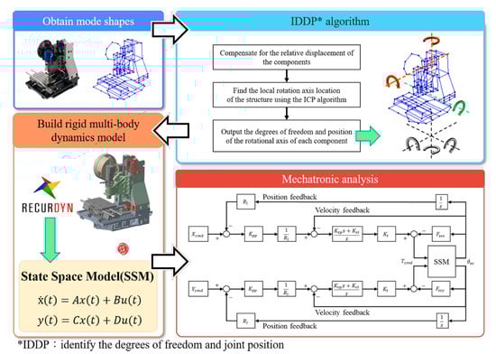
Figure 1. Overall research process.

The remainder of this paper is organized as follows. Section 2 introduces the proposed modeling process and algorithms. Section 3 validates the models identified by the proposed method. Section 4 applies the identified model to perform mechatronic integration analysis and provides and discusses the results. Finally, Section 5 concludes the paper.

2. Proposed Identification of DOF and Joint Position Process

The machine in this study is a three-axis vertical machining center. This serial structure of machine is widely used [19]. To omit the tedious FE model building process, a virtual model was constructed with a bottom-up approach. As a result, a simplified model with minimum DOFs was built. The model can provide sufficient information on the relative motion between the tool center point (TCP) and the machine tool table. The machining center was operated without large deformation due to mutual perpendicularity of the feeding directions. Therefore, low variations in the natural frequency and vibration pattern in a small range of motion could be assumed. Because the proposed method could identify the structure of non- feed drive systems, the entire machine structure was divided into two parts, the casting and the feed drive system, as shown in Figure 2. The modeling method for the feed drive system is quite mature and has been proposed by many scholars [20,21,22,23]. In this study, the modeling was performed using four DOFs. As shown in the figure, $K_C$ is the torsional stiffness between the motor and the coupling. $K_S$ and $C_S$ are the axial stiffness and damping between the coupling and the ball screw, respectively. $K_T$ and $C_T$ are the stiffness and damping between the table and the saddle, respectively. The casting system was analyzed using the proposed identification of DOF and joint position (IDDP) process. The following illustrates the approach to construct a virtual model by selecting DOF information from the mode shape, as shown in Figure 3.

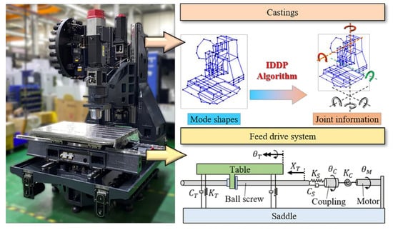
Figure 2. Structural classification.

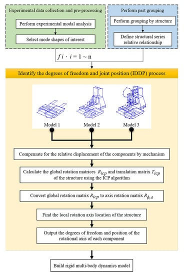
Figure 3. Flowchart of the IDDP.

Step 1: Experimental data collection and pre-processing. Perform EMA was conducted to obtain the frequency response function (FRF) for the structure. The natural frequency ($f_i$) and mode shape were selected (Section 2.1).

Step 2: Component grouping. The model analyzed was a series-type mechanism. It was necessary to find the relative relationship between the components to compensate for the relative displacement of the components through the mechanism (Section 2.2).

Step 3: Perform IDDP process. After the data point group was compensated, the rotational matrix of the data point group was analyzed using the ICP algorithm to find the rotational axis by inverse operation. Then, the position of the rotational axis in space was calculated to obtain the position and DOF of the joint between the two parts in the rigid multi-body dynamics model (Section 2.3).

2.1. Modal Information Acquisition

The first step was to find the natural frequencies and mode shapes. An impact testing was used to obtain this modal information. The mode shapes were obtained from the imaginary part of the FRF, which is introduced in Section 3.

2.2. Component Grouping and Relative Displacement Compensation

In the series mechanism, if the rotational axis and position of the absolute coordinates are found using the ICP method without compensating for the displacement of the previous object (Figure 4a), such an approach can cause errors in model setup. Therefore, to find the DOFs of the relative motion of each pair of objects (Figure 4b), displacement compensation was required for the mode shape of each mode in each model before the analysis. Structure grouping was needed before the displacement compensation to define the relative relationship of the series mechanism. The CNC vertical machining center machine tool can be regarded as a series mechanism, which includes the following three models in the structure: (1) Model 1, which includes the base and the X- and Y-axis feed drive systems; (2) Model 2, which consists of Model 1 with a column and the Z-axis feed drive system; and (3) Model 3, which consists of Model 2 with the tool magazine, as shown in Figure 5. Then, the relative displacement compensation was conducted.

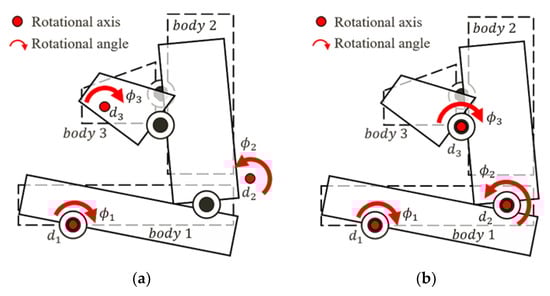
Figure 4. Rotational axes found by using different coordinates: (a) absolute; (b) relative.

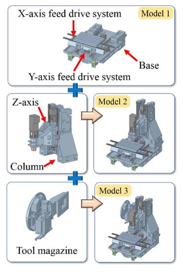
Figure 5. Structural grouping and series relationship.

The relative transformation, such as the translation, rotational angle, and rotational axis between the two bodies, was found by canceling the former bodies’ transformation. The bodies in a series mechanism were numbered in a bottom-up manner. For example, the former bodies of Body 3 were coded as Body 1 and Body 2.

The mechanism’s kinematics was derived using a displacement matrix. Then, the transformation was reversed to cancel the former bodies’ transformation (Figure 6). A displacement matrix E was the matrix that was transformed for the body from one location to another with respect to a fixed coordinate, which is denoted as

$$E\left(\varphi ,d,T\right)=\left[\begin{array}{cc}{R}_{\left(\varphi ,d\right)}& T\\ 0& 1\end{array}\right]$$

(1)

where $R_{(\varphi , d)}$ is an axial rotation matrix and T is a prismatic translation vector.

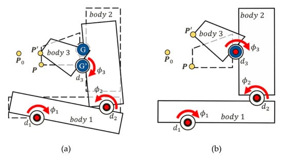
Figure 6. Canceling the former transformation: (a) mode shape before cancelation; (b) mode shape after cancelation.

The location of the point $P$ on the end body $i$ was described by the displacement matrix $E_{0i}$ and an arbitrary initial location $P_0$ as

$$P=E_{0i}{P}_0$$

(2)

Similarly, the new location $P^{\prime }$ can be described as

$$P^{\prime }=E_{0i}^{\prime }{P}_0$$

(3)

To cancel the previous transformation, the point of interest G was the connection point between body i and body i − 1. The purpose is to find the transformation matrix such $E_{{\mathrm{GG}}^{\prime }}$ that the point $G$ can be transformed to the point $G^{\prime }$.

$$G^{\prime }=E_{G{G}^{\prime }}G$$

(4)

Equations (2) and (3) were used to express the transformation matrix in Equation (4) as

$$E_{G{G}^{\prime }}=E_{0\left(i-1\right)}^{\prime }{\left(E_{0\left(i-1\right)}\right)}^{-1}$$

(5)

The matrices $E_{0(i-1)}$ and $E_{0(i-1)}^{\prime }$ can be denoted as

$$\begin{gathered} E_{0\left(i-1\right)}=E_{01}{E}_{{12}_{{\left(0,d,T\right)}_1}}{E}_{{23}_{{\left(0,d,T\right)}_2}}\cdots E_{{\left(i-2\right)\left(i-1\right)}_{{\left(0,d,T\right)}_{i-1}}} \\ {E}_{0\left(i-1\right)}^{\prime }=E_{01}^{\prime }{E}_{{12}_{{\left(\varphi ,d,T\right)}_1}}^{\prime }{E}_{{23}_{{\left(\varphi ,d,T\right)}_2}}^{\prime }\cdots E_{{\left(i-2\right)\left(i-1\right)}_{{\left(\varphi ,d,T\right)}_{i-1}}}^{\prime } \end{gathered}$$

(6)

Through the above derivations, the point $G^{\prime }$ can be transformed back to point $G$, meaning that “the former transformation is cancelled,” as mentioned previously. Finally, the relative transformation can be found by conducting ICP with the new point set ${\mathbb{G}}_i^{\prime }$.

2.3. Finding the Position and DOF of Rotational Axis

Arbitrary movement of an object in space can be represented by rotation and translation vectors. The rotation and translation matrices found by the ICP method are calculated based on a global origin of coordinate, but the location of the rotational axis cannot be used to build a model. Therefore, a solution was proposed. In Section 2.3.1, the ICP algorithm is explained, and the rotation matrix is converted into an axial rotation matrix to solve the vector of the rotational axis. Then, Section 2.3.2 describes the approach to find the position of the rotational axis between the components by the proposed algorithm. Through the above process, the position and vector of the rotational axis between the two components can be obtained.

2.3.1. Calculation of Rotation Axial Vectors

To automatically and quickly determine the change of the mode shape, the rigid transformation matrix was found by applying the ICP algorithm to the group of accelerated gauge measurement points and converting them into an axial rotation matrix to obtain the rotation axial vector and the rotation angle.

The ICP [24] is a well-known method to realize point cloud registration, a process of finding a spatial transformation from one point cloud to another. The purpose is to merge the point clouds of multiple views into a complete model globally. Thus, the aim is to register a measured point set $\mathbb{P}=\left\{p_i\right\}$ to a model point set $\mathbb{Z}=\left\{z_i\right\}$. A mean square objective function to be minimized can be defined as the following function:

$$M\left(q\right)=\frac{1}{N_p}{\displaystyle \sum }_{i=1}^{N_p}||z_i-R\left(q_R\right)p_i-q_T||{}^2$$

(7)

where $R\left(q_R\right)$ is a rotation matrix generated by a unit rotation quaternion $q_R$, and $q_T$ is a translation vector. The complete registration state vector $q$ is denoted as $q= {\left[q_R{/q}_T\right]}^T$.

For each clustered point set ${\mathbb{S}}_i$, the rigid transformation matrix $R\left(q_R\right)$ with rotation and/or translation transformation for every natural frequency is given by the ICP algorithm.

$$R\left(q_R\right)=\left[\begin{array}{ccc}{q}_0^2+q_1^2-q_2^2-q_3^2& 2\left(q_1{q}_2-q_0{q}_3\right)& 2\left(q_1{q}_3+q_0{q}_2\right)\\ 2\left(q_1{q}_2+q_0{q}_3\right)& q_0^2+q_2^2-q_1^2-q_3^2& 2\left(q_2{q}_3-q_0{q}_1\right)\\ 2\left(q_1{q}_3-q_0{q}_2\right)& 2\left(q_2{q}_3+q_0{q}_1\right)& q_0^2+q_3^2-q_1^2-q_2^2\end{array}\right]$$

(8)

The rotational matrix can be represented in the axial rotation matrix form $R_{(\varphi ,d)}$ rotated around any axis as follows:

$$R\left(q_R\right)=R_{\left(\varphi ,d\right)}=\left[\begin{array}{ccc}{d}_x^{2}V\varphi +c\varphi & d_y{d}_{x}V\varphi -d_{z}n\varphi & d_z{d}_{x}V\varphi +d_{y}n\varphi \\ d_x{d}_{y}V\varphi +d_{z}n\varphi & d_y^{2}V\varphi +c\varphi & d_z{d}_{y}V\varphi -d_{x}n\varphi \\ d_x{d}_{z}V\varphi -d_{y}n\varphi & d_y{d}_{z}V\varphi +d_{x}n\varphi & d_z^{2}V\varphi +c\varphi \end{array}\right]=\left[\begin{array}{ccc}{a}_{11}& a_{12}& a_{13}\\ a_{21}& a_{22}& a_{23}\\ a_{31}& a_{32}& a_{33}\end{array}\right]$$

(9)

where $V\varphi =1-cos\varphi$, $c\varphi =cos\varphi$, $n\varphi =sin\varphi$, and $a_{ij}$(i = 1, 2, 3, j = 1, 2, 3) is a pure quantity parameter calculated by Equation (8).

The rotational angle ($\varphi$) and the rotational unit vector ($d_x,d_y,d_z$) can be solved by the following equations:

$$\begin{gathered} \varphi =|\pm {\cos }^{-1}\frac{a_{11}+a_{22}+a_{33}-1}{2} \\ {d}_x|=\frac{a_{32}-a_{23}}{2n\varphi } \\ {d}_y|=\frac{a_{13}-a_{31}}{2n\varphi } \\ {d}_z|=\frac{a_{21}-a_{12}}{2n\varphi } \end{gathered}$$

(10)

2.3.2. Center of Rotation Position of Object

The ICP algorithm can find the vector of the rotational axis between two components. The vector is the global reference coordinates relative to the transform point sets, and this coordinate point position cannot be used in modeling. To solve this problem, a procedure is proposed to find the position of the transformation point sets as described below.

For any point $g$ in the point set ${\mathbb{G}}_i$, a displacement vector $r$ is defined as

$$r=g^{\prime }-g$$

(11)

where $g^{\prime }$ is the displaced point of a mode shape. For each two displacement vectors $r_1$ and $r_2$, a normal vector $w$ is defined as

$$w=r_1\times r_2$$

(12)

Then, the two perpendicular bisectors of $r_1$ and $r_2$ can be found by passing the vectors $w\times r_1$ and $w\times r_2$ through the midpoints of $r_1$ and $r_2$, respectively. The perpendicular bisectors, $r_1$ and $r_2$, are coplanar.

The above procedure is repeated for every two displacement vectors. An arbitrary plane normal to the rotational axis is found, and all the perpendicular bisectors are projected to the plane. Then, the highest density point of the stiffness points can be found (Figure 7). Finally, the point is reversed from the normal plane to a three-dimensional space. As shown in Figure 8, the rotational axis is assumed to pass through the intersection, which is the set position of the joint.

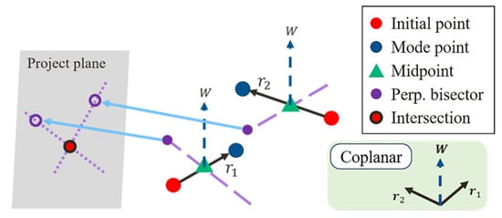
Figure 7. Project the perpendicular bisectors to the normal plane.

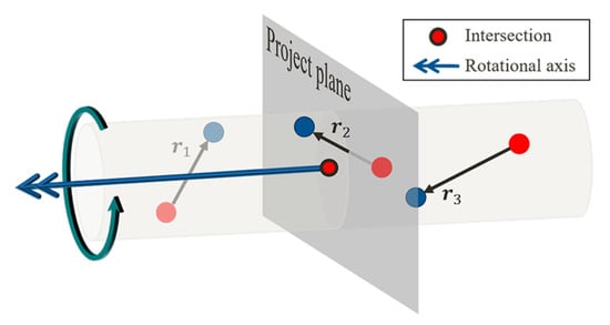
Figure 8. Invert the rotational point to 3-D coordinate.

3. Simulation Analysis and Verification of Experimental Results

3.1. Construction of Vertical Machine Center Model

To understand the vertical processing machine natural frequency and mode shape, impact testing was carried out according to the entire machine structure combined with EMA, as shown in Figure 9. The impact hammer excited the machine structure to obtain the natural frequency of the structure. Experiments were performed by moving the accelerometer to each measurement location and applying impact loadings to the fixed location in different directions. Three impact loadings were applied to each measurement location to collect three signals, which were averaged to reduce experimental error. Table 1 shows the specifications of the equipment used in the impact testing. The measurements of frequency ranged from 0 to 150 Hz. Figure 10 shows the FRF’s imaginary part of 131 measurement locations, including the x, y, and z directions. The concentrated peak value of the curve was the natural frequency. The peak value was the vector value of the mode shape. The proposed identification method used these data in analysis. The low-frequency vibration of the machine had a great impact on machining quality. Therefore, this study focused on the natural frequencies below 100 Hz. In addition, significant modes were selected by calculating the relative displacement between the table and the TCP. The modes having only small displacements between the table and the TCP were ignored. Finally, six mode shapes with natural frequencies of 21, 26.5, 31.5, 38, 44, and 58 Hz were selected as the basis for building the simplified model, as shown in Figure 11.

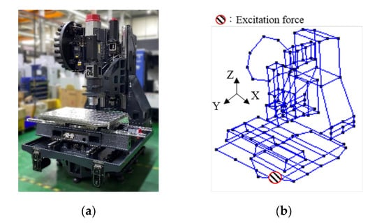
Figure 9. Vertical machining center: (a) experimental model; (b) EMA model.

Table 1. Equipment parameters for impact testing.

Name	Type	Sensitivity	Unit
Impact Hammer	PCB 086D20	0.2237	mV/N
Accelerometers (X)	ICP 356A02	9.76	mV/g
Accelerometers (Y)		9.86	mV/g
Accelerometers (Z)		9.68	mV/g

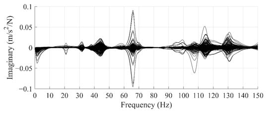
Figure 10. Frequency response function.

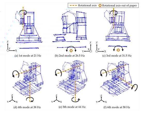
Figure 11. Experimental with the first six natural frequencies and mode shapes.

3.2. IDDP Process

The following describes the IDDP process performed by a vertical machine:

Step 1: Perform part grouping. The structural grouping of the entire machine model and the definition of the series relationship are shown in Figure 5.

Step 2: Find the rotational axis. The IDDP was carried out according to the mode shape of each natural frequency. With the base as an example, the 26.5-Hz mode shape data were selected for IDDP analysis to calculate the rotational axis. Each frequency was analyzed sequentially. The frequency analysis results of each mode are shown in Figure 12a.

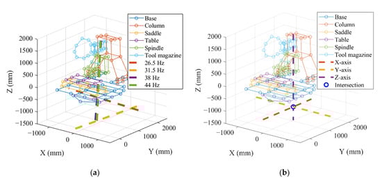
Figure 12. IDDP results for base: (a) total rotational axes for each frequency; (b) the intersection for the joint position.

Step 3: Find the joint location. The rotational axis found by each mode does not define the position of the joint. Therefore, the repeated rotational axes of the same dimension were averaged to obtain the DOF of the base and the position of the rotational axis, as shown in Figure 12b.

Through the proposed IDDP method, the DOFs of the entire machine were identified. The DOFs of the feed drive system were compiled, and the entire machine model had 18 DOFs, as shown in Table 2. Table 3 shows the joint location found by the IDDP method. All position values are based on the origin of the global coordinate,${ O}_G$. The identified joint DOFs are described below:

Table 2. Joint’s DOF of entire model.

Part		Translation	Rotation
Casting	Base	0	3
	Column	0	1
	Tool magazine	0	2
Feed drive system	X-axis	1	3
	Y-axis	1	3
	Z-axis	1	3
Subtotal		3	15
Total			18

Table 3. Joints setting position.

Part	X (mm)	Y (mm)	Z (mm)
Base	0	1063	−1500
Column	0	1300	100
Tool magazine	−280	1500	1350

• The base has three DOFs and is set up as a spherical joint at the point $O_F$:

  (a)

  Base rotation around the X-axis corresponds to the Base Pitch.

  (b)

  Base rotation around the Y-axis corresponds to the Base Roll.

  (c)

  Base rotation around the Z-axis corresponds to the Base Yaw.

• The column has one DOF and is set up as cylindrical joint at the point $O_{C,B}$:

  (a)

  Column rotation around the X-axis corresponds to the Column Pitch.

• The tool magazine has two DOFs and is set up as a universal joint at the point $O_{T,C}$:

  (a)

  Tool magazine rotation around the Y-axis corresponds to the Tool Magazine Roll.

  (b)

  Tool magazine rotation around the Z-axis corresponds to the Tool Magazine Yaw.

The above three types of joints all restricted linear DOF. $O_B$, $O_C$, and $O_T$ are the centers of mass for the base, column, and tool magazine respectively, which are connected with the corresponding joint points. The joint was set in the multi-body dynamics software RecurDyn to constrain the corresponding DOF and rotational stiffness, as shown in Figure 13. The joint stiffness values are shown in Table 4. Finally, a modal analysis was carried out to verify the natural frequency and the mode shape.

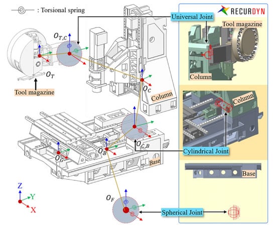
Figure 13. Dynamic model with identified joints.

Table 4. Joint stiffness for each part in the movement dimension.

Joint	Stiffness (GN-mm/rad)
Base Roll	653.58
Base Yaw	147.12
Base Pitch	902.78
Column Pitch	184.64
Tool magazine Roll	2.68
Tool magazine Yaw	5.56

3.3. Modal Analysis

Dynamic characteristics are important for the dynamic behavior. The dynamic characteristics of the simplified model can be verified by comparing the natural frequencies and the mode shapes. The dynamic characteristics are affected by the identified joint location and stiffness. Table 5 shows the comparison of the experimental and simulated natural frequencies with a maximum error of 4.8%. Figure 14 shows the corresponding mode shapes for each natural frequency. Each simulated mode shape was consistent with the experimental mode shape, showing that the dynamic characteristics of the simplified model are accurate.

Table 5. Comparison of natural frequencies between experiment and simulation.

Mode	1	2	3	4	5	6
EMA (Hz)	21	26.5	31.5	38	44	58
Simplified model (Hz)	21.5	26.4	32.8	39.8	44.4	58
Error (%)	2.4	0.2	4.1	4.8	1	0

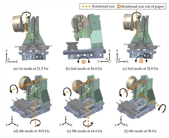
Figure 14. Simulated with the first six natural frequencies and mode shapes.

4. Case Study of Motion Path Simulation

4.1. Servo Simulation Model of Mechatronics System

The model created by the proposed method can be integrated into the servo control loop for mechatronic integration simulation. Figure 15 shows the block diagram of the entire control loop. The model has a PI controller, which is a closed loop system. First, the position command ($X_{\mathsf{cmd}}, Y_{\mathsf{cmd}}$), which is obtained by the actual controller monitoring function, is input. The position command passes the proportional gain $K_{\mathsf{pp}}$ in the position loop and the proportional gain $K_{\mathsf{vp}}$ and integral gain $K_{\mathsf{vi}}$ in the velocity loop. $R_l$ converts rotation into translation motion. It is calculated by the ball screw pitch divided by 2π. Then, the motor constant $K_t$ converts the angular velocity into torque ($T_{cmd}$), which is input to each axis motor of the virtual model (SSM) to make the machine move. During the movement, the changes in motor angular velocity are fed back to the position and speed loops, respectively. The servo parameters are obtained from an actual controller. Meanwhile, considering the friction effect in the structure, the angular velocity ${\dot{\theta }}_{ec}$ of the motor is substituted into the friction function ($F_{ssx}, F_{ssy}$) to calculate the friction force, which is combined with the motor torque into the torque that considers the friction. An adopted LuGre friction model [25] is shown in Figure 16, and it can be constructed by recording the motor torque at different constant velocities [14]. The friction model is described as follows:

$$F_{ss}\left({\dot{\theta }}_{ec}\right)=F_{c}sgn\left({\dot{\theta }}_{ec}\right)+\left(F_s-F_c\right)e^{-{\left(\frac{{\dot{\theta }}_{ec}}{{\alpha }_s}\right)}^2}sgn\left({\dot{\theta }}_{ec}\right)+{\tau }_2{\dot{\theta }}_{ec}$$

(13)

where $F_{ss}\left({\dot{\theta }}_{ec}\right)$ is the steady-state friction function, ${\dot{\theta }}_{ec}$ is the angular velocity, $F_c$ is the Coulomb friction force, $F_s$ is the static friction force, ${\alpha }_s$ is the Stribeck angular velocity, and ${\tau }_2$ is the viscous coefficient. The system parameters in the mechatronic system are shown in Table 6.

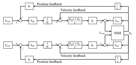
Figure 15. Block diagram of controller and the proposed machine tool model.

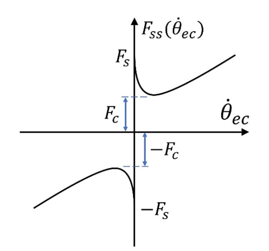
Figure 16. The steady-state friction function.

Table 6. System parameters in mechatronic system.

Symbol	Value	Symbol	Value
$K_{pp}$	60 (1/s)	${\tau }_{2\mathsf{x}}$	0.1 (N·m/(rad·s−1))
$K_{vp}$	0.0766 (A·s/m)	${\alpha }_{\mathrm{sx}}$	0.5 (rad/s)
$K_{vi}$	3.8282 (A/m)	$F_{cy}$	0.0069 (N·m)
$R_l$	0.001591 (m/rad)	$F_{sy}$	1.3374 (N·m)
$K_t$	15.1 (N/m)	${\tau }_{2\mathsf{y}}$	0.16 (N∙m/(rad·s−1))
$F_{cx}$	0.0115 (N·m)	${\alpha }_{\mathrm{sy}}$	0.5 (rad/s)
$F_{sx}$	4.7318 (N·m)

4.2. State-Space Model Setup

After the model was set up in the multi-body dynamics software, to perform the analysis more directly with Matlab, the multi-body dynamics model was converted into a multi-input and multi-output SSM. Its mass, stiffness, damping matrices, and user-defined control I/Os (Equation (14)) can be computed with built-in functions to obtain the state-space matrix.

$$\begin{gathered} \dot{x}\left(t\right)=Ax\left(t\right)+Bu\left(t\right) \\ y\left(t\right)=Cx\left(t\right)+Du\left(t\right) \end{gathered}$$

(14)

where x(t) is the state vector; u(t) is the input vector; y(t) is the output vector; A is the system matrix; B is the input matrix; C is the output matrix; and D is the forward transmission matrix.

4.3. Motion Trajectory Result Validation

The servo loop model was verified through the line–curve hybrid trajectory, which was run at the feed rate of 4000 mm/min. A cross grid encoder was used to measure the two-dimensional relative displacement of the table and the TCP, which had a 1-nm resolution. The experimental setup is shown in Figure 17. Figure 18 shows the generated torque command. The blue line represents the experimental torque command, and the red dashed line represents the simulated torque command. The figure clearly shows that the simulated and experimental torque results are very consistent. Figure 19 shows the experimental and simulated line–curve hybrid trajectories. Based on the contour error results, regardless of the vibration cusp of the angle of a straight line or the commutation cusp of an arc, the experimental and simulated results were very similar. These results show that the proposed model can accurately predict the dynamic error trend of the machine tool.

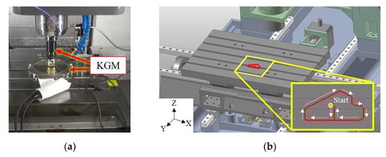
Figure 17. Motion trajectory: (a) KGM cross grid mounted on the machining center; (b) simulation.

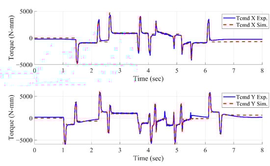
Figure 18. Comparison between measured and simulation torque.

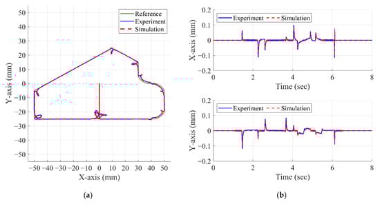
Figure 19. Comparison between measured and simulation result: (a) line–curve hybrid trajectory with 50 times the error; (b) x- and y-axis contour error.

5. Conclusions

This paper proposed a new method of establishing a virtual model of an entire machine by identifying the mode vectors. The virtual model with only 18 DOFs was established effectively. This method is suitable for series structures. The joint position and DOF of the joint between two components in the rigid multi-body dynamics model were obtained by automatically identifying the mode vectors. The natural frequency and mode shape of the mathematical model were verified by modal analysis, and the maximum error in frequency prediction was 4.8%. The simulated mode shapes were consistent with the experimental results. Finally, the series controller and the mathematical model were used for mechatronic integration analysis. The established model can completely simulate the motion trajectory’s errors. This accurate and efficient virtual model can be easily combined with intelligent diagnosis calculations on a computer associated with a machine or on the cloud. The proposed model can be applied to (a) health monitoring, fault diagnosis, and failure prognosis techniques for mechanical components (e.g., linear guide or bearing wear can be diagnosed by a change in a specific mode shape), (b) servo tuning control strategies (e.g., adjust the gain value in the control loop and observe the effect on the trajectory to select the best control strategy for machining), and (c) workpiece surface quality prediction (e.g., when the machining path changes, the machined surface quality can be predicted by observing the relative displacement of the worktable and the TCP during the movement of the machine).

References

- Altintas, Y.; Brecher, C.; Weck, M.; Witt, S. Virtual machine tool. CIRP Ann. 2005, 54, 115–138. [Google Scholar] [CrossRef]
- Zatarain, M.; Lejardi, E.; Egana, F.; Bueno, R. Modular synthesis of machine tools. CIRP Ann. 1998, 47, 333–336. [Google Scholar] [CrossRef]
- Zhuang, Z.W.; Lu, J.C.; Liu, D.S. A novel identification technique of machine tool support stiffness under the variance of structural weight. Int. J. Adv. Manuf. Technol. 2022, 119, 247–259. [Google Scholar] [CrossRef]
- Ealo, J.A.; Garitaonandia, I.; Fernandes, M.H.; Hernandez-Vazquez, J.M.; Muñoa, J. A practical study of joints in three-dimensional Inverse Receptance Coupling Substructure Analysis method in a horizontal milling machine. Int. J. Mach. Tools Manuf. 2018, 128, 41–51. [Google Scholar] [CrossRef]
- Deng, C.; Yin, G.; Fang, H.; Meng, Z. Dynamic characteristics optimization for a whole vertical machining center based on the configuration of joint stiffness. Int. J. Adv. Manuf. Technol. 2015, 76, 1225–1242. [Google Scholar] [CrossRef]
- Chen, H.; Tan, Z.; Tan, F.; Yin, G. Dynamic performance analysis and optimization method of the horizontal machining center based on contact theory. Int. J. Adv. Manuf. Technol. 2020, 108, 3055–3073. [Google Scholar] [CrossRef]
- Craig, R.R., Jr.; Bampton, M.C. Coupling of substructures for dynamic analyses. AIAA J. 1968, 6, 1313–1319. [Google Scholar] [CrossRef]
- Bilgili, D.; Budak, E.; Altintas, Y. Multibody dynamic modeling of five-axis machine tools with improved efficiency. Mech. Syst. Sig. Process. 2022, 171, 108945. [Google Scholar] [CrossRef]
- Duan, M.; Lu, H.; Zhang, X.; Li, Z.; Zhang, Y.; Yang, M.; Liu, Q. Dynamic modeling and experimental research on position-dependent behavior of twin ball screw feed system. Int. J. Adv. Manuf. Technol. 2021, 117, 3693–3703. [Google Scholar] [CrossRef]
- Brussel, H.V.; Sas, P.; Nemeth, I. Towards a mechatronic compiler. IEEE/ASME Trans. Mechatron. 2001, 6, 90–105. [Google Scholar] [CrossRef]
- Garitaonandia, I.; Fernandes, M.H.; Albizuri, J. Dynamic model of a centerless grinding machine based on an updated FE model. Int. J. Mach. Tools Manuf. 2008, 48, 832–840. [Google Scholar] [CrossRef]
- Zaeh, M.; Siedl, D. A new method for simulation of machining performance by integrating finite element and multi-body simulation for machine tools. CIRP Ann. 2007, 56, 383–386. [Google Scholar] [CrossRef]
- Lee, C.H.; Yang, M.Y.; Oh, C.W.; Gim, T.W.; Ha, J.Y. An integrated prediction model including the cutting process for virtual product development of machine tools. Int. J. Mach. Tools Manuf. 2015, 90, 29–43. [Google Scholar] [CrossRef]
- Huang, H.W.; Tsai, M.S.; Huang, Y.C. Modeling and elastic deformation compensation of flexural feed drive system. Int. J. Mach. Tools Manuf. 2018, 132, 96–112. [Google Scholar] [CrossRef]
- Wang, C.P.; Erkorkmaz, K.; McPhee, J.; Engin, S. In-process digital twin estimation for high-performance machine tools with coupled multibody dynamics. CIRP Ann. 2020, 69, 321–324. [Google Scholar] [CrossRef]
- Sato, R.; Tashiro, G.; Shirase, K. Analysis of the coupled vibration between feed drive systems and machine tool structure. Int. J. Autom. Technol. 2015, 9, 689–697. [Google Scholar] [CrossRef]
- Sato, R.; Ito, Y.; Mizuura, S.; Shirase, K. Vibration Mode and Motion Trajectory Simulations of an Articulated Robot by a Dynamic Model Considering Joint Bearing Stiffness. Int. J. Autom. Technol. 2021, 15, 631–640. [Google Scholar] [CrossRef]
- RecurDyn, V9R5; FunctionBay, Inc.: Seongnam-si, Korea. 2022. Available online: http://dev.functionbay.com/RecurDynOnlineHelp/V9R5/index.html# (accessed on 22 October 2022).
- Lyu, D.; Liu, Q.; Liu, H.; Zhao, W. Dynamic error of CNC machine tools: A state-of-the-art review. Int. J. Adv. Manuf. Technol. 2020, 106, 1869–1891. [Google Scholar] [CrossRef]
- Altintas, Y.; Verl, A.; Brecher, C.; Uriarte, L.; Pritschow, G. Machine tool feed drives. CIRP Ann. 2011, 60, 779–796. [Google Scholar] [CrossRef]
- Frey, S.; Dadalau, A.; Verl, A. Expedient modeling of ball screw feed drives. Prod. Eng. 2012, 6, 205–211. [Google Scholar] [CrossRef]
- Vicente, D.A.; Hecker, R.L.; Villegas, F.J.; Flores, G.M. Modeling and vibration mode analysis of a ball screw drive. Int. J. Adv. Manuf. Technol. 2012, 58, 257–265. [Google Scholar] [CrossRef]
- Liu, Y.; Feng, X.; Li, P.; Li, Y.; Su, Z.; Liu, H.; Lu, Z.; Yao, M. Modeling, Identification, and Compensation Control of Friction for a Novel Dual-Drive Hydrostatic Lead Screw Micro-Feed System. Machines 2022, 10, 914. [Google Scholar] [CrossRef]
- Besl, P.J.; McKay, N.D. Method for registration of 3-D shapes. Sensor fusion IV: Control paradigms and data structures. Int. Soc. Opt. Photonics 1992, 1611, 586–606. [Google Scholar] [CrossRef]
- Johanastrom, K.; Canudas-De-Wit, C. Revisiting the LuGre friction model. IEEE Control Syst. Mag. 2008, 28, 101–114. [Google Scholar] [CrossRef]
Publisher’s Note: MDPI stays neutral with regard to jurisdictional claims in published maps and institutional affiliations. |
© 2022 by the authors. Licensee MDPI, Basel, Switzerland. This article is an open access article distributed under the terms and conditions of the Creative Commons Attribution (CC BY) license (https://creativecommons.org/licenses/by/4.0/).