Article

Residual-Electrical-Endurance Prediction of AC Contactor Based on CNN-GRU

Key Lab of Special Electric Machine and High Voltage Apparatus, College of Electrical Engineering, Shenyang University of Technology, Shenyang 110870, China
*
Author to whom correspondence should be addressed.
Machines 2022, 10(11), 1067; https://doi.org/10.3390/machines10111067
Submission received: 30 August 2022 / Revised: 3 November 2022 / Accepted: 8 November 2022 / Published: 11 November 2022
(This article belongs to the Section Electrical Machines and Drives)

Abstract

:
AC contactors are used frequently in various low-voltage control lines, so remaining-life prediction for them can significantly improve the operational reliability of power control systems. To address the problem that the existing AC contactor remaining-life prediction methods do not make full use of the correlation between previous and later states in the degradation process, a CNN-GRU (convolutional neural network-gated recurrent unit) method for AC-contactor remaining-life prediction is proposed. Firstly, the entire cycle of an AC contactor’s degradation data is obtained through a whole-life test, from which the characteristic parameters that effectively reflect the operating states of the contactor are extracted; secondly, neighborhood component analysis (NCA) and maximal information coefficient (MIC) are used to eliminate the redundant information of multidimensional parameters in order to select the optimal feature subset; and then, CNN is used to compress the feature dimension and mine the regular information between the features, so as to extract the effective feature vectors; finally, taking the AC contactor remaining electrical life as a long time sequence issue, time-series accurate prediction is performed using GRU. It is verified that this model is better than RNN (recurrent neural network), LSTM (long short-term memory) and GRU models in prediction, with an effective accuracy of 96.63%, which effectively supports the feasibility of time-series prediction in the field of the remaining-life prediction of electrical devices.

1. Introduction

The main functions of AC contactors are turning on and off the high-current main circuits frequently, which are widely used in low-voltage control systems [1]. With the maturity of online monitoring technology, it is obvious that AC contactors tend to be more and more intelligent. The online collection and intelligent analysis of AC-contactor operating parameters can provide the scientific basis for equipment maintenance [2]. The residual electrical endurance of AC contactors reflects the line on–off performance, and if it can be predicted in time before failure, it can significantly improve the reliability of power systems and reduce economic losses [3].
Considering the importance of AC contactors to power systems, researchers have conducted in-depth studies on the prediction of the residual-electrical-endurance of AC contactors in recent years. M. Zong et al. solved the voltage switching problem for AC-3 and AC-4 operating conditions using PLC and a new type of transformer to improve the test accuracy, where AC-3 operating condition means to turn on and off the circuit at 0.17 times of the rated voltage and 1 time of the rated current, and AC-4 operating condition means to turn on and off the circuit at 1 time of the rated voltage and 6 times of the rated current [4]. Z. Wu et al. proposed a modeling method for the residual-electrical-endurance prediction of AC contactors based on conditional density estimation, which can achieve high accuracy [5]. S. Kumari et al. estimated the health status of AC contactors using the relationship between feature parameters such as contact resistance and residual-electrical-endurance [6]. Z. Wu et al. used control strategies to improve the electrical life of AC contactors by studying the relationship between arc phase angle, arc energy and contact mass loss [7]. S. Zheng et al. simulated electrical-endurance distribution characteristics based on a contact ablation model and they evaluated the reliability of AC contactors using electrical endurance tests [8]. H. Cui et al. used a convolutional neural network (CNN) to build an electrical-endurance-prediction model by extracting the signals of voltage and current waveforms, and they used a voting mechanism to improve the prediction accuracy [9]. S. Sun et al. calculated Euclidean distance based on the correlation of statistical indicators and the initial feature parameters, and residual-electrical-endurance prediction was performed using a one-dimensional regression model [10]. K. Li et al. established Wiener degradation model by constructing normally distributed degradation variables, and they validated the method by simulating residual-electrical-endurance tests using the Monte Carlo method [11]. S. Abirami et al. established a stochastic gradient-descent classifier model to estimate the residual-electrical-endurance prediction using operational data under different operating conditions [12].
However, unfortunately, the following problems were ignored in the above investigations for predicting the residual-electrical-endurance of AC contactors: (1) Only a few feature parameters were adopted, and the degradation information could not be represented effectively, which affects the accuracy of prediction results. (2) The electrical condition monitoring signal is non-linear and non-smooth, and with the increase in feature parameters, the regular information between multiple feature parameters and the residual-electrical-endurance prediction cannot be explored efficiently. (3) The electrical endurance of AC contactors was not considered as a long time-series problem, and it was not fully considered that the residual-electrical-endurance is determined by both the current and previous states, and the relationship between the states before and after the degradation process could not be utilized effectively, which further restricts the improvement in prediction precision.
With the rise of artificial-intelligence technology, machine learning [13] and deep-learning [14] have been widely applied in electrical engineering. Among them, deep-learning can directly model and analyze the degradation data of electrical equipment without the need for accurate physical models and statistical models of degradation, which are suitable for solving the problem of the residual-electrical-endurance prediction of complex electrical equipment.
The convolutional neural network (CNN) and recurrent neural network (RNN) are important components of deep-learning. CNN is a deep feedforward neural network with powerful feature-extraction capability, which is widely used in vibration-signal feature extraction [15], and image feature extraction [16], etc. RNN allows the network to have a “memory” function by preserving the information in the implicit layers, thus allowing it to adapt to the analysis of time-series data [17]. Long short-term memory (LSTM) introduces a “gate” structure based on RNN, which can effectively improve the gradient-disappearance and gradient-explosion problems caused by the long-term dependence of RNN by controlling the process of information flow into the cell state [18]. Gated recurrent unit (GRU) simplifies the original input gate, forgetting gate and output gate into update gate and reset gate on the basis of LSTM, and the calculation of hidden states are improved, which not only reduces the computational complexity but also reduces the risk of overfitting [19]. GRU timing-prediction models are widely used in the field of remaining-life prediction for bearings [20], and lithium batteries [21], etc. However, AC contactors have a large number of feature covariates, and too many features will make the neural network training difficult and even mean overfitting will occur, which will affect the accuracy of prediction; therefore, preliminary feature screening is necessary for the accuracy of final prediction.
Based on the above analysis, this work constructed a residual-electrical-endurance prediction model for an AC contactor based on the CNN-GRU method. This model regards the life state of the AC contactor as a time-series degradation, and fully considers the correlation between the front and back states of the multi-feature parameters in the time dimension. Firstly, the optimal feature subset was selected by NCA and MIC to characterize the degradation information of the AC contactor effectively. Secondly, the CNN was used to extract the effective feature vector, and the regular information between the features is deeply excavated. Finally, GRU was used to fully consider the correlation of the previous and later states and memorize the information of the long-time history features to achieve the time-series prediction of the residual-electrical-endurance of AC contactors. The results of the case analysis show that the prediction method has high precision, which provides a new method for the residual-electrical-endurance prediction of switchgear appliances.

2. Principles

The theories applied in this investigation include NCA, MIC, CNN and GRU.

2.1. Neighbor Component Analysis

NCA is an embedded feature-selection method which calculates the similarity based on the Mahalanobis distance, which selects the nearest neighbors randomly by learning the feature weights and minimizing the objective function and uses the leave-one-out method to cross-validate the original data set to achieve feature selection [22]. The calculation procedure of NCA feature selection are as follows [23].
(1) The transformation matrix A is set up and the Mahalanobis distance between features is calculated. For the n samples in data set { X 1 , X 2 , , X n } , the Mahalanobis distance between sample points X i and X j is expressed as:
d i s t m a h X i , X j = A X i A X j T A X i A X j
where i , j = 1 , 2 , , n .
(2) The formulae for calculating the probability of a single feature data which is classified correctly are as follows:
P i j = exp A X i A X j 2 l i exp A X i A X l 2 , P i i = 0
P i = j W i P i j
where l is the set of samples excluding sample X i ; P i j is the probability of the effect of sample X j on sample X i ; P i is the accuracy of the leave-one-out method for sample X i ; and W i is the set of subscripts belonging to the same class of samples as X i .
(3) The transformation matrix A is optimized and take derivative of the target function taken; the formulas are as follows:
f ( A ) = i = 1 n P i = i = 1 n j W i P i j
f ( A ) A = 2 A i n j W i P i j X i j X i j T k P i k X i k X i k T
where k = 1 , 2 , , n , X i j = X i X j .
(4) Using the optimized transformation matrix to achieve feature selection for the original feature matrix X , the feature subset X ˜ is expressed as:
X ˜ = X A

2.2. Maximal Information Coefficient

The maximum information coefficient (MIC) based on mutual information (MI) theory was presented first by D. N. Reshef et al. in 2011, which is believed to be an excellent indicator to measure the correlation between variables [24]. MI is based on the marginal probability density and joint probability density of random variables, which represents the similarity of information between two random variables X and Y. The higher the similarity between X and Y, the larger the value of MI. MI is calculated by entropy value. When a variable X has a probability distribution p ( X = x ) , its entropy value can be expressed as:
H ( X ) = x p ( X = x ) log 2 p ( X = x )
The MI I ( X , Y ) of two variables, X and Y, are defined as follows:
I ( X , Y ) = x X y Y p ( x , y ) log p ( x , y ) p ( x ) p ( y )
where p ( X , Y ) is the probability density of the joint distribution of the two random variables X and Y. The marginal probabilities of X and Y are p ( X ) and p ( Y ) , respectively.
The MIC method divides the scatter plot of two variables X and Y into multiple regions and calculates the mutual information for the data in each region and uses the maximum value of the mutual information as the MIC value between the variables. For the data set D of two variables, the formula for calculating the maximum information coefficient is expressed as:
MIC ( D ) = max X Y < B ( n ) M ( D ) X , Y = max X Y < B ( n ) I ( D , X , Y ) log ( min ( X , Y ) )
where n is the sample size and B ( n ) is the maximum grid number, which is generally taken as B ( n ) = n 0.6 [25].

2.3. Convolutional Neural Network

As shown in Figure 1, the structure of a CNN mainly includes an input layer, a convolutional layer, a pooling layer, a fully connected layer and an output layer [26]. The structural layers are equivalent to filters between them, which can remove the noise from the feature data effectively. The main computational steps of a CNN are shown below.
(1) The convolution layer is the core of the CNN in which the convolution calculation realizes local perception and weight sharing through feature mapping. The formula is expressed as:
y j l = f i M j x i l 1 ω i j l + b i l
where y j l is the jth feature mapping in the lth layer of the current layer; f ( · ) is the activation function; M j is the input feature map; x i l 1 is the ith feature map of the previous layer; ω i j l is the convolution kernel of the ith layer and the jth layer; and b i l is the bias.
(2) The pooling layer, also called the down-sampling layer, is used to reduce the number of parameters and prevent overfitting and generally using maximum pooling. The formula is expressed as:
S k max - pooling   = max a l ( i , t )
where S k max - pooling is the value of the corresponding neuron after pooling; and a l ( i , t ) is the output of the tth neuron of the ith mapping in the lth layer.
(3) The fully connected layer reduces the network dimension and outputs the feature vector, which can be expressed as:
h x l = f ω x l 1 + b
where h x l is the fully connected output of the lth layer; ω is the weight of the neuron node; x l 1 is the fully connected input of the lth layer; and b is the bias parameter.

2.4. Gated Recurrent Unit

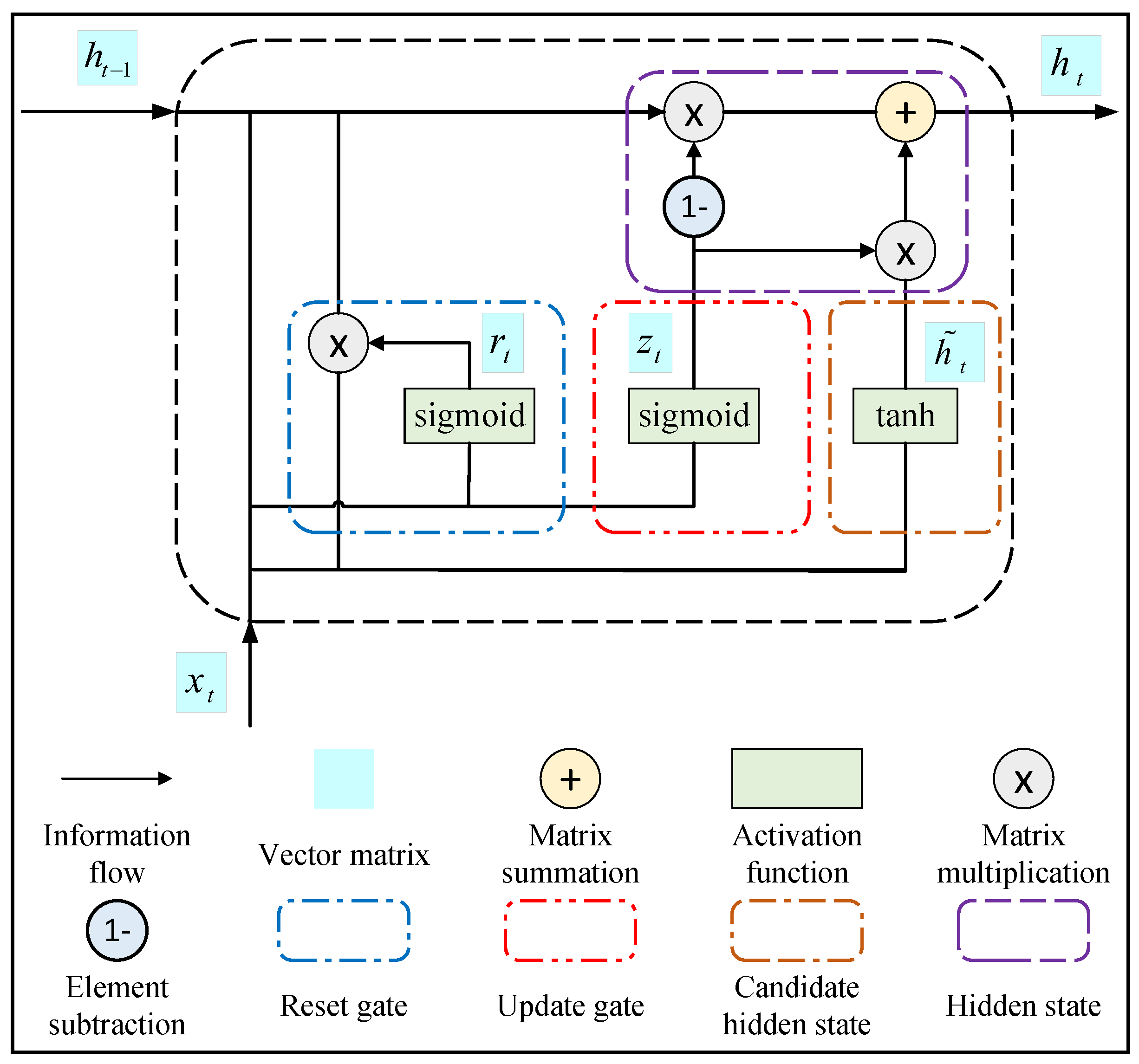
The internal structure of a GRU is shown in Figure 2 [27]. The reset gate r t and the update gate z t in the GRU are the input x t of the current time step and the hidden state h t 1 of the previous time step, which are calculated by the sigmoid activation function in the fully connected layer. The formulas are as follows:
r t = σ x t W x r + h t 1 W h r + b r
z t = σ x t W x z + h t 1 W h z + b z
The more state information of the previous moment is brought into the current state with the larger the update gate z t , the less the information of the previous state is written into the current candidate set h ˜ t and the smaller the reset gate r t .
The candidate hidden state h ˜ t in the GRU is an element-wise multiplication of the output of the reset gate r t at the current time step with the hidden state h t 1 at the previous time step, which is calculated by connecting the input of the current time step x t and the output of the element multiplication in the fully connected layer of the tanh activation function. The calculation formula is expressed as:
h ˜ t = tanh x t W x h + r t h t 1 W h h + b h
The hidden state h t in the GRU is calculated by calculating the hidden state h t 1 of the previous time step and the candidate hidden state h ˜ t of the current time step through the update gate z t . The formula is as follows:
h t = z t h t 1 + 1 z t h ˜ t
where W x r , W x z , W h r , W h z , W h x and W h h are the weight parameters and b r , b z and b h are the deviation parameters. As described above, the process of the GRU neural network can be simplified and expressed as:
h t = GRU x t , h t 1
The circular structure of a GRU is shown in Figure 3, which extends the feature information through multiple GRU modules to achieve the prediction of long-time sequences.

3. Prediction Model

3.1. Overview of Prediction Model

This paper is based on the CNN-GRU residual-electrical-endurance prediction model of the AC contactor. The structure of this model is shown in Figure 4.
Firstly, the AC contactor full-life test platform is built, and the voltage and current signals during operation are collected using high-precision sensors to extract the feature parameters which reflect the degradation state of the AC contactor. Then, NCA is used to calculate the importance of the feature parameters to the residual-electrical-endurance, and the optimal feature subset is obtained by removing the invalid and redundant feature parameters to the residual-electrical-endurance prediction with the correlation degree of the feature parameters, which are calculated by MIC. After that, the optimal feature subset is subjected to dimensionless normalization. The processed multidimensional time series are input into the CNN, and the feature vectors are extracted by setting the CNN model structure, and the number and size of convolutional kernels. Mining the regular information between features by using the depth of convolutional computation, and compressing the feature dimension by using the maximum pooling operation, can retain the feature information and further reduce the complexity of computation. Finally, the extracted feature vectors are extended and input into the GRU, and the remaining number of operations of AC contactors is used as the prediction label to set the window length and divide the data set. The GRU neural network is trained by setting the GRU model structure and hyperparameters, initializing the network parameters, and continuously updating the weights and biases. The GRU fully considers the correlation before and after the AC contactor life cycle and captures the sequence long-time step dependence while taking account of the correlation and nonlinear relationship of the time-series data, which can efficiently remember the long-time history feature information and output them through the fully connected layer. The predicted values are back-normalized to obtain the results of the predicted remaining number of operations, and the predicted results are evaluated and analyzed using evaluation indexes.

3.2. Model Loss-Function and Evaluation Index

The Adam optimizer is selected in this paper to optimize the model parameters during the training of the prediction model, which optimizes the loss-function while improving the convergence of the model [28]. The prediction model in this paper uses the mean squared error (MSE) function as the loss-function, which is expressed in the following formula.
Loss = 1 n t = 1 n y t y ^ t 2
where n is the number of samples; y t is the actual value and y ^ t is the predicted output value of the model.
Meanwhile, in order to evaluate the advantages and disadvantages of the prediction results, the root mean square error (RMSE), the mean absolute error (MAE) and the goodness of fit ( R 2 ) were selected to evaluate the prediction results. The formulas are as follows:
RMSE = 1 n t = 1 n y ^ t y t 2
MAE = 1 n t = 1 n y ^ t y t
R 2 = t = 1 n y ^ t y ¯ 2 t = 1 n y t y ¯ 2 = 1 t = 1 n y t y ^ t 2 t = 1 n y t y ¯ 2
where y ^ is the average of the actual value. RMSE reflects the extent to which the data deviates from the true value; MAE reflects the size of the error and R 2 represents the extent to which the independent variable reflects the dependent variable. The smaller the RMSE and MAE are, the higher the R 2 is, and the better the prediction effect and the performance of the model will become.

4. Experimental Design and Feature Extraction

4.1. Construction of Test Platform

The AC contactor full-life test platform was built and tested according to the on–off test requirements specified in [29]. In practical applications, the AC contactor mainly operates under the working condition of AC-4; that is, the on-off circuit is connected at 1 time of the rated voltage and 6 times of the rated current. Meanwhile, the contact of the AC contactor is ablated seriously and the performance degradation trend is obvious under the condition of AC-4. Therefore, the experiment condition of AC-4 was selected for this test. The specific parameters are shown in Table 1.
In the table, I is the making current; I e is the rated operational current; U is the external voltage; U e is the rated operational voltage; I c is the breaking current and U r is the rated frequency resume voltage.
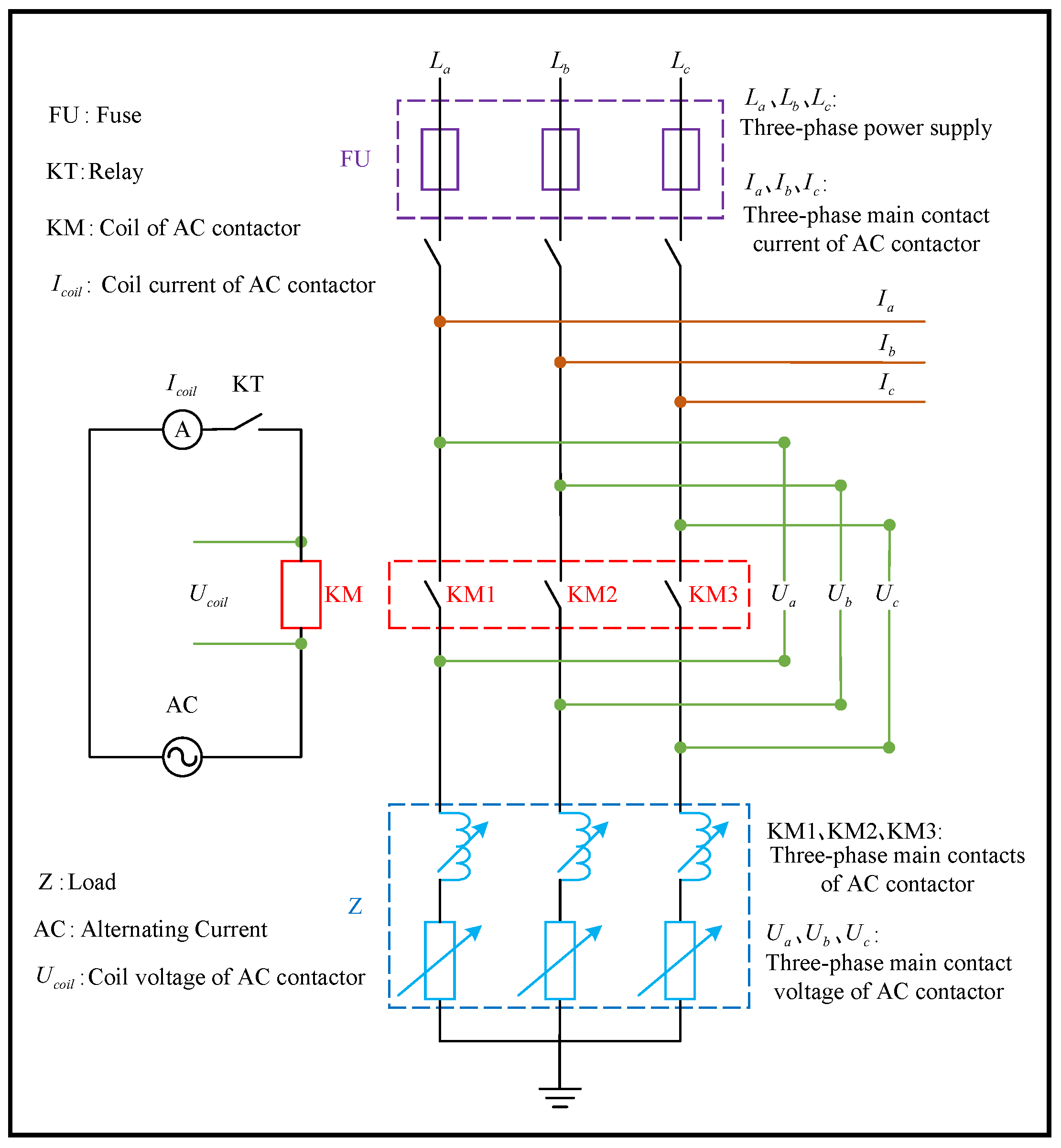
The construction of the AC contactor full-life test platform includes hardware circuit design and software procedure design. The schematic diagram of the hardware circuit is shown in Figure 5 and the electrical diagram of the main circuit is shown in Figure 6.
Through the X series USB6356 data acquisition card of the NI company and the voltage and current sensor of the Lime company, the three-phase main-contact voltage, three-phase main-contact current, coil voltage and current during the breaking and closing process of the AC contactor were collected. The technical parameters of the sensor are shown in Table 2.
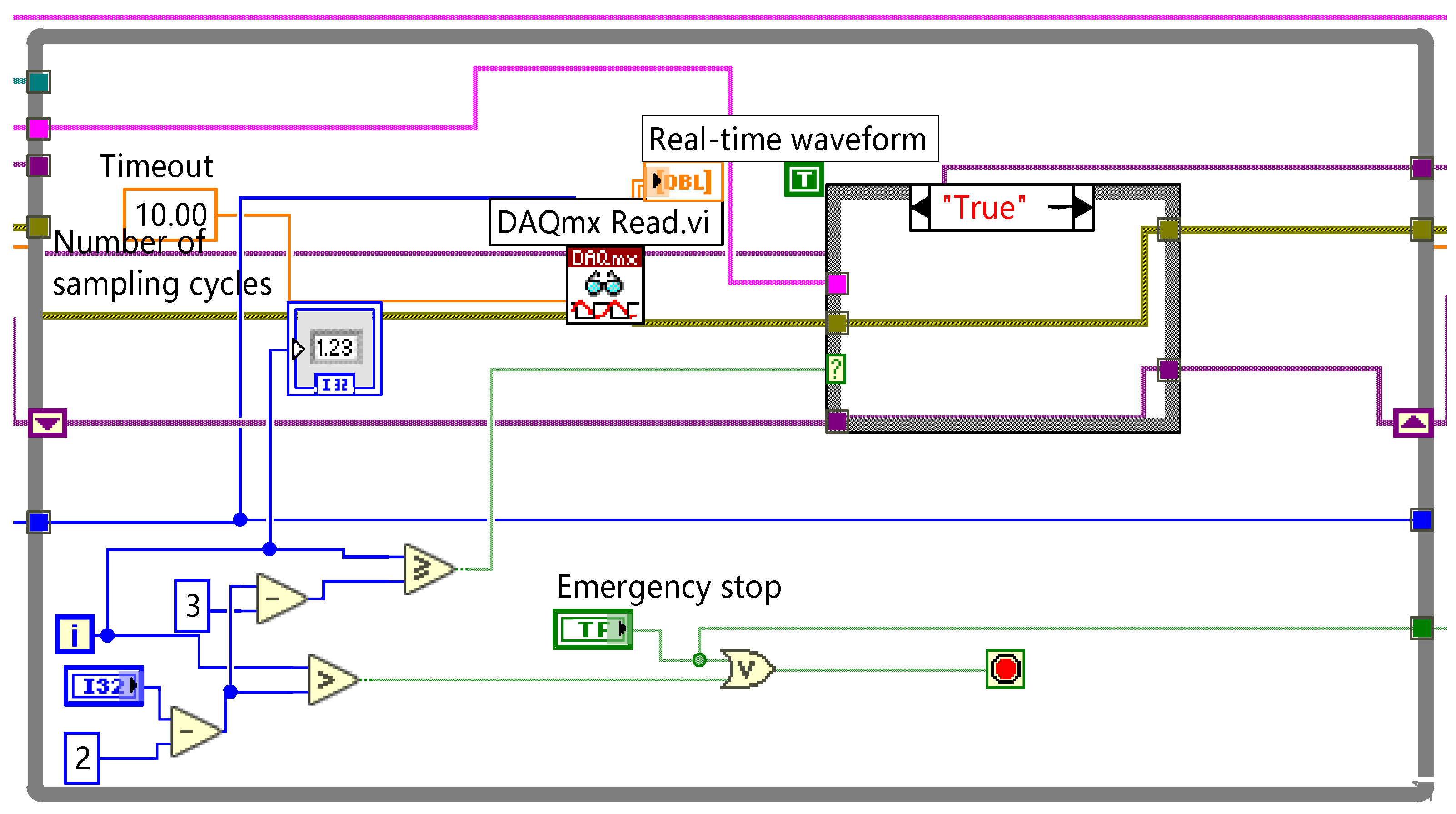
The software programming combines the NI data-acquisition card with LabVIEW through the communication serial port to realize the online acquisition of the running data. The LabVIEW front-end control panel is shown in Figure 7. The program diagram of the LabVIEW back-end is shown in Figure 8.
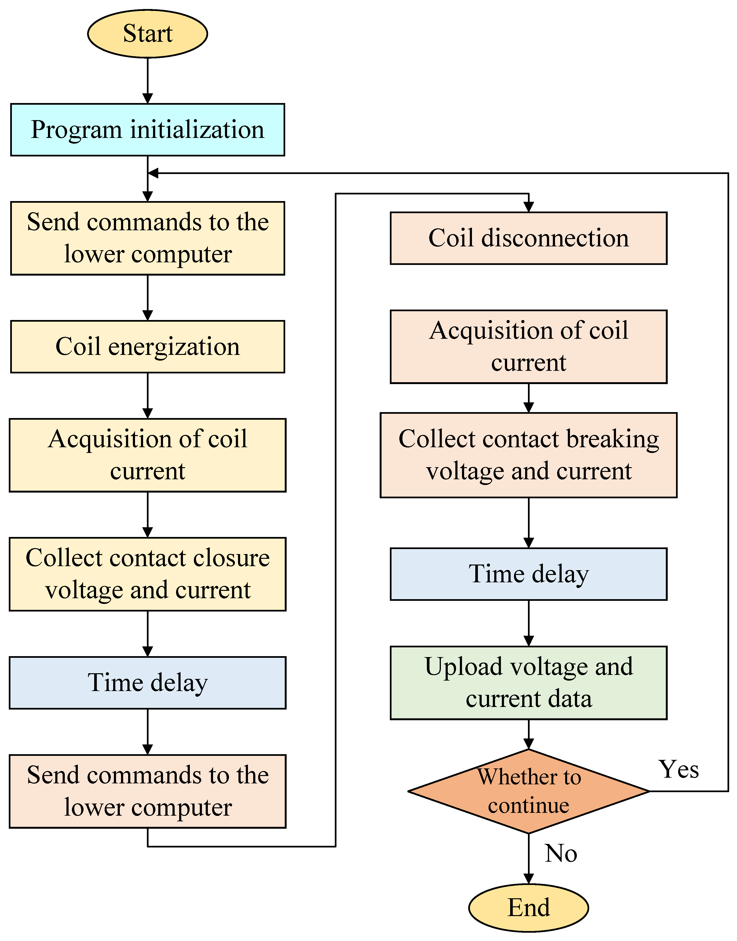
The flow chart of the software control of the test system is shown in Figure 9. After initialization, the program sends a closing command to the lower computer, and the microcontroller receives the command and outputs a high-level signal to control the relay to close, and then the contactor coil is energized to turn on the main circuit. Over a span of time, the contactor is disconnected from the main circuit by sending a break command to the lower computer. The waveform data of the test is collected, displayed and saved in real time.
Finally, the schematic diagram of the physical principle of the AC contactor full-life test platform is shown in Figure 10.

4.2. Extracting Feature Parameters

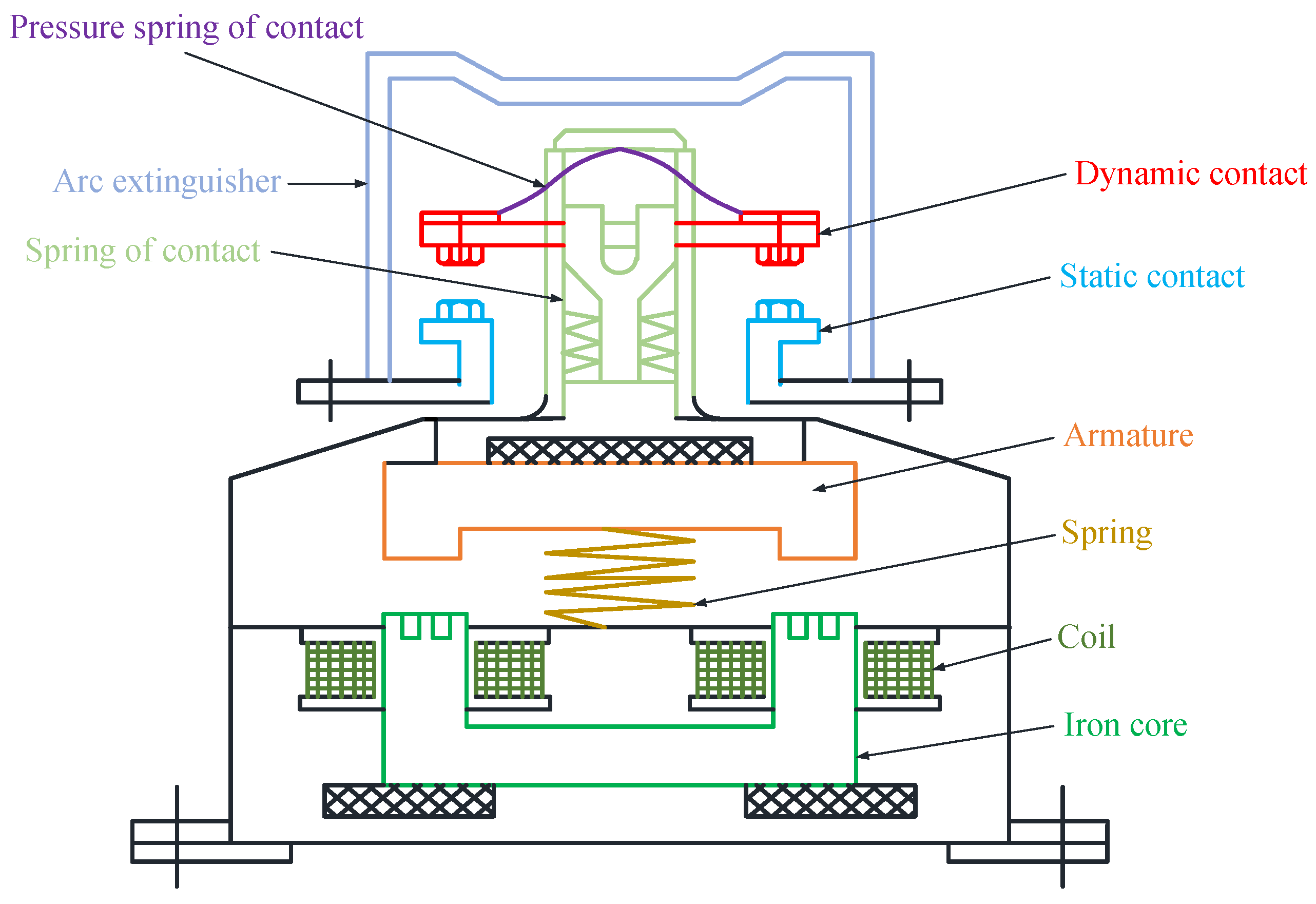
The basic construction of the AC contactor is shown in Figure 11.
The arc generated during the breaking and closing of the stationary and moving contacts of the AC contactor will cause the electrical wear and fusion welding of the contacts, thus affecting the electrical conductivity of the electrical contacts and the residual-electrical-endurance of the AC contactor.
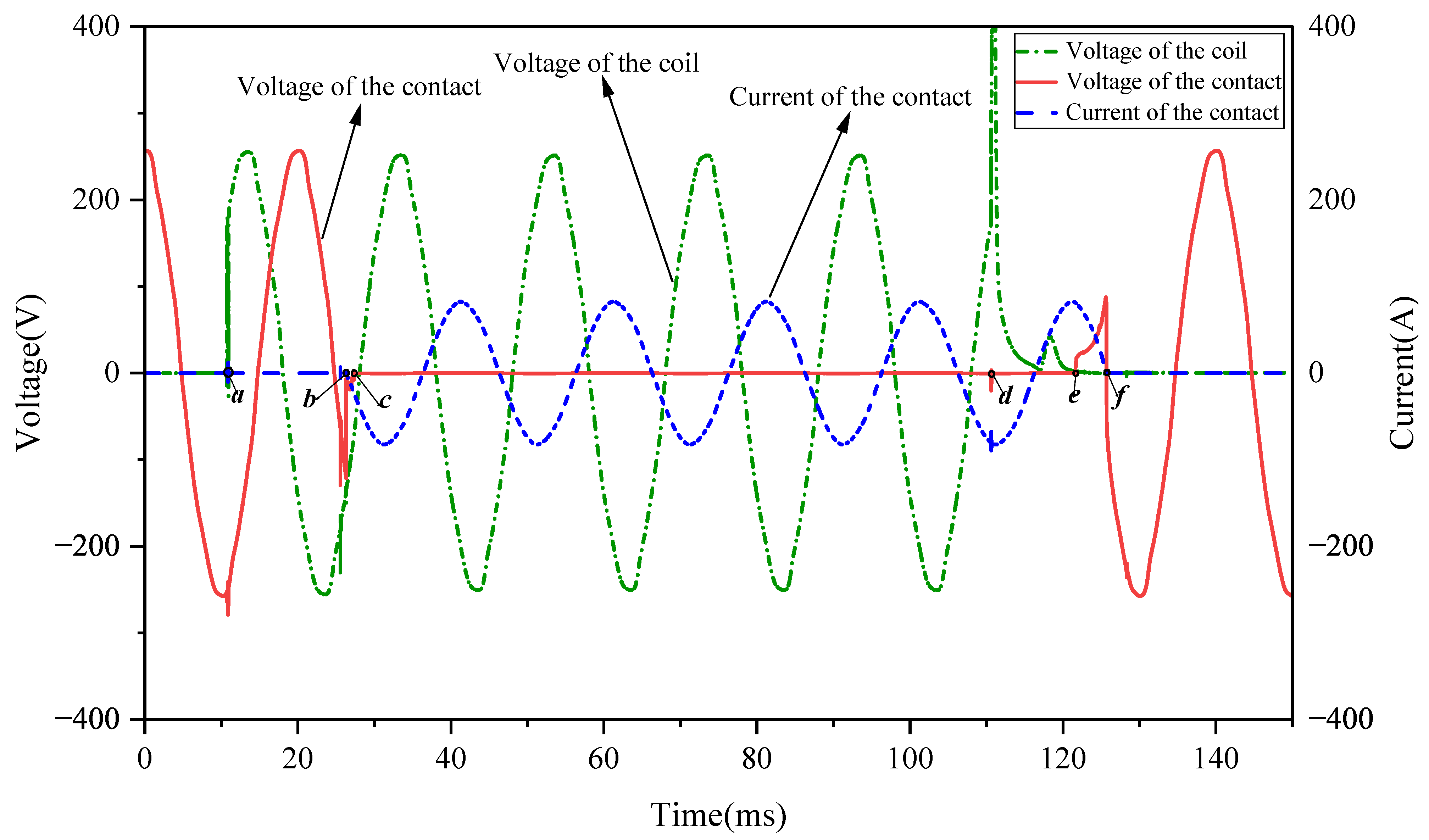
By collecting the contact voltage, contact current and contactor coil voltage waveforms, the feature parameters can be extracted, which can characterize the life degradation state of the AC contactor effectively. The normal breaking and closing waveform of the AC contactor is shown in Figure 12.
The specific moment point states during the AC contactor’s breaking and closing are shown in Table 3.
The characteristic parameters of the AC contactor are calculated according to the characteristic principle of the AC contactor using the state of the contact at each moment, combining the sampling frequency and the information of the contact voltage and current. The contact resistance is the additional resistance present at the contact between the two contacts, i.e., the root mean square value of the voltage and current under one cycle of stable contact energization. The period between the coil being energized and the movable and static contacts making first contact is defined as the pull-in time. The period between energizing the coil and the first contact of the moving and static contacts is defined as the bounce time. The period between when the arc is generated and when the arc is extinguished is defined as the arcing time. The energy generated by the arc during one breaking process is defined as the arc burning energy, which is obtained by discretization of voltage and current signals, in practice. Average arc power refers to the average power of the arc energy during the arcing time. The period between the coil de-energizing and the moving and static contacts separating is defined as the release time. The specific equations for AC-contactor characteristic parameters were calculated on the basis of Figure 12 and Table 3, as shown in Table 4 [30].
In the table: u j is the contact voltage; i j is the contact current; N is the number of sampling points; Δ t is the sampling interval time and f s is the sampling rate.

5. Case Analysis

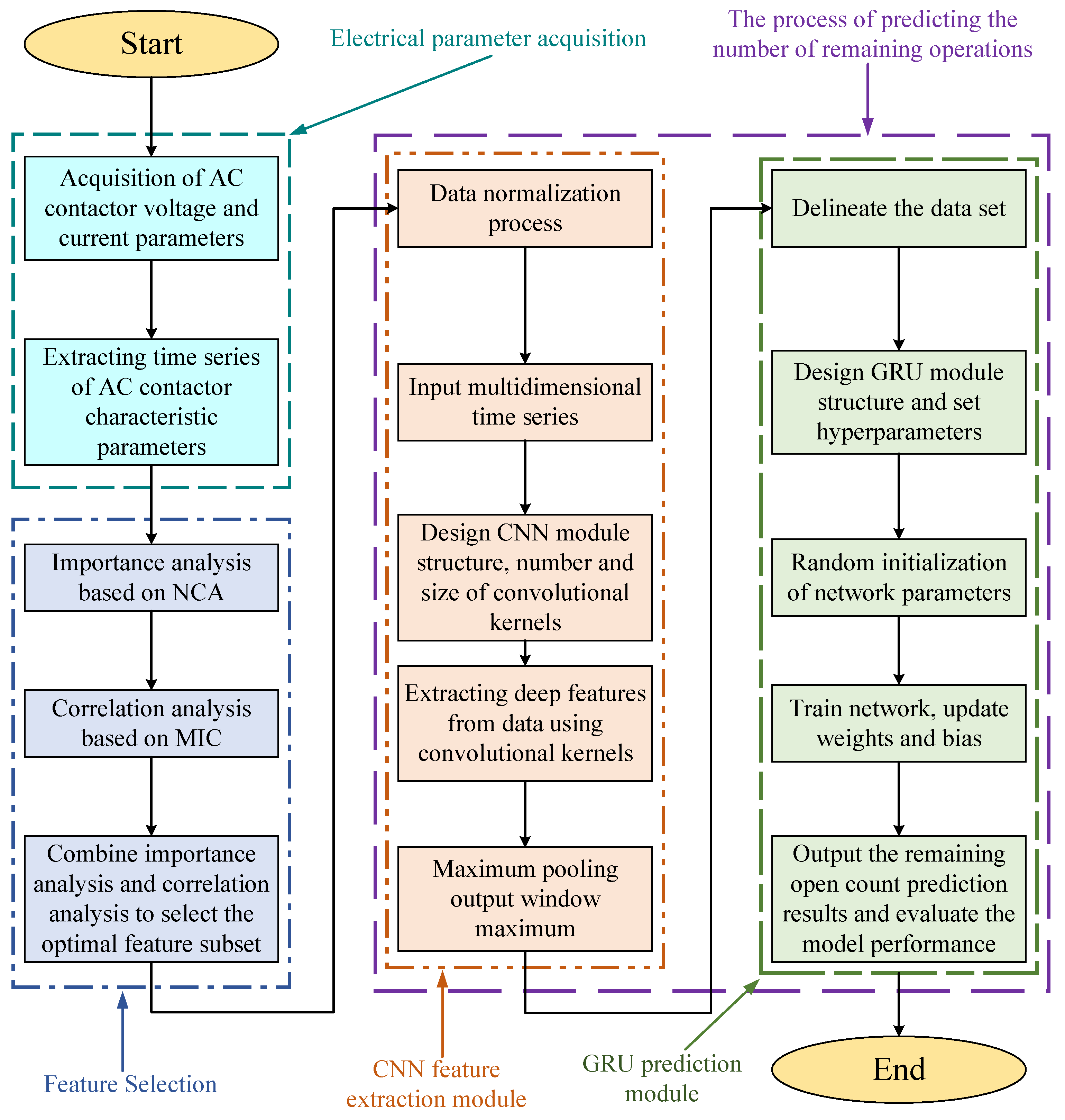
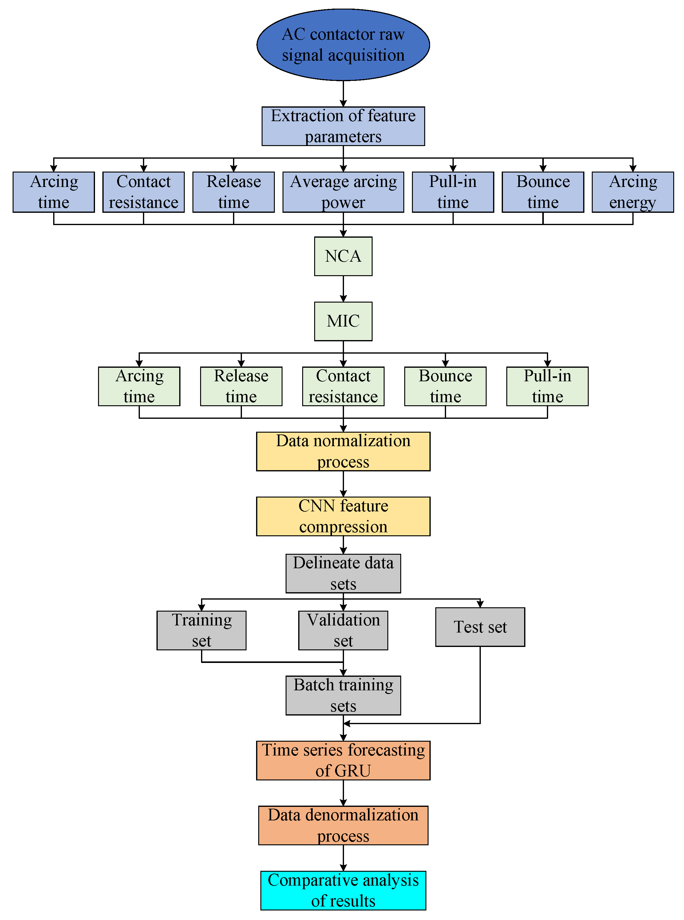
The flow chart of the case analysis is shown in Figure 13. Firstly, the voltage and current signals were collected through the full-life test platform of the AC contactor, and the feature parameters of the AC contactor were extracted. Secondly, the optimal feature subset was selected using NCA feature importance analysis and MIC. Thirdly, the optimal feature subset was normalized and input into the CNN for feature compression and dimension reduction. Fourthly, the remaining operations of the AC contactor were used as prediction labels to construct and divide the data set. Finally, the data set was input into the GRU neural network for time-series prediction, and the prediction result was output after inverse normalization.

5.1. Feature Parameter Extraction

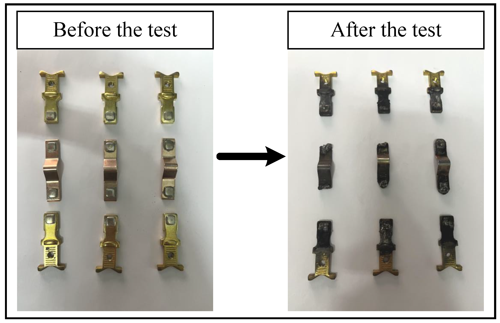
In order to prove the feasibility and accuracy of the method in this paper, the CJX2–8011 AC contactor was used for verification, and a comparison of the three-phase contact ablation before and after the sample test is shown in Figure 14.
From the comparison, one can see that when the electrical life of the AC contactor is terminated, the three-phase contacts are severely ablated. The original sequences of the feature parameters of the test samples and their variation trends are shown in Figure 15.

5.2. Feature Parameters Selection

Although rich feature parameters can reflect the actual degradation information of AC contactors, too many feature parameters will contain a large amount of redundant information, which not only increases the complexity of model calculation but also affects the accuracy of residual-electrical-endurance prediction; therefore, the extracted feature parameters need to be filtered [31].
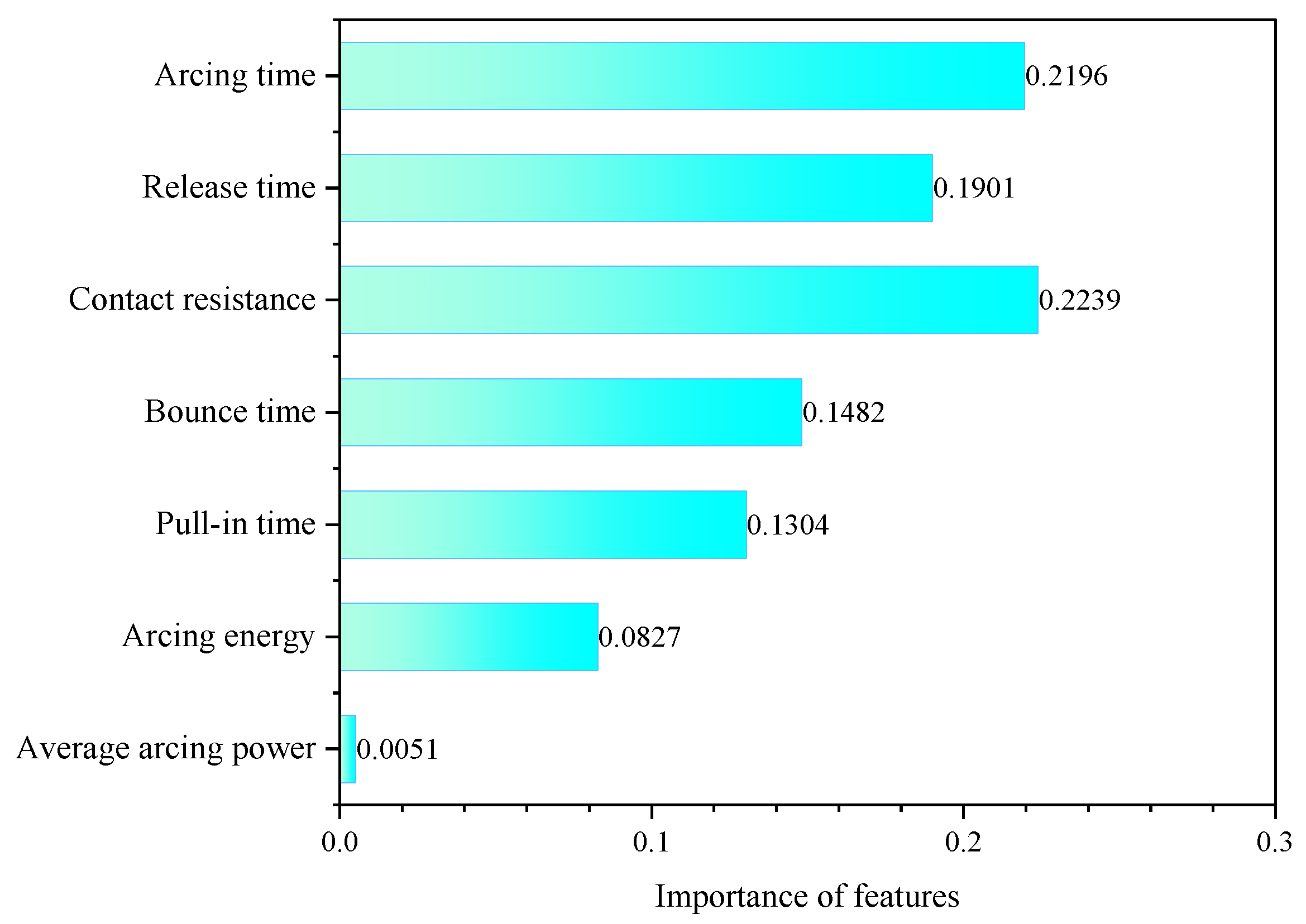
In this paper, the importance of the feature parameters on the residual-electrical-endurance and the correlation between the features are considered, and the NCA and MIC are combined to select the optimal feature subset. The importance of the feature parameters on the residual-electrical-endurance is calculated using NCA feature importance analysis, which is shown in Figure 16.
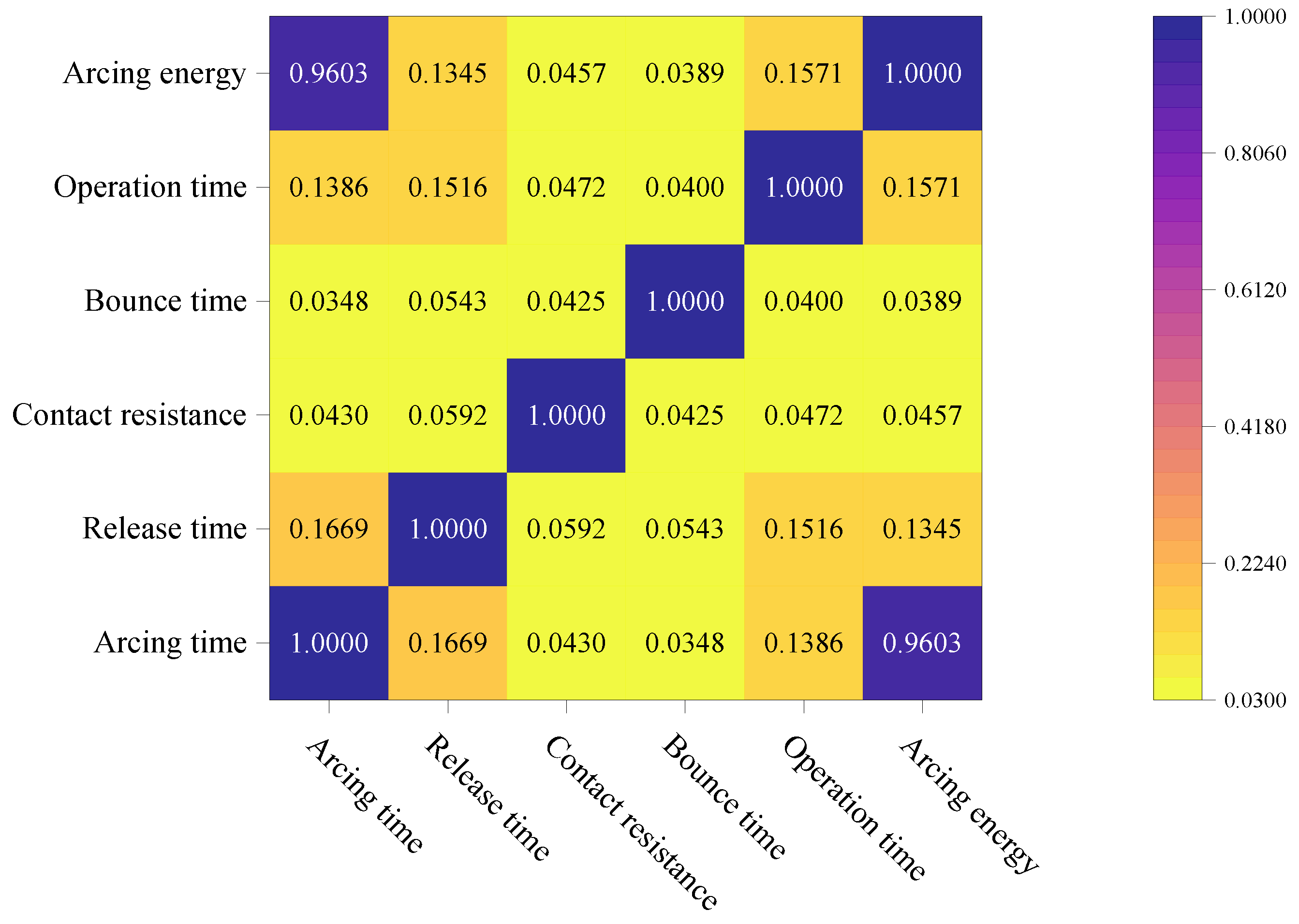
Through the NCA feature importance analysis, the mean arc power has the lowest importance for the residual-electrical-endurance, and should be eliminated. After that, the correlation coefficients among the remaining six feature parameters were calculated using MIC, and the correlation coefficient heat map is shown in Figure 17.
The MIC heat map shows that the arc duration and the arc energy are strongly correlated, and the feature information is extremely similar. The arc duration is retained according to the importance analysis results.
In summary, this paper selects contact resistance, arc duration, release time, pull-in time and bounce time as the optimal subset of feature parameters of the model input.

5.3. Model Parameters Setting

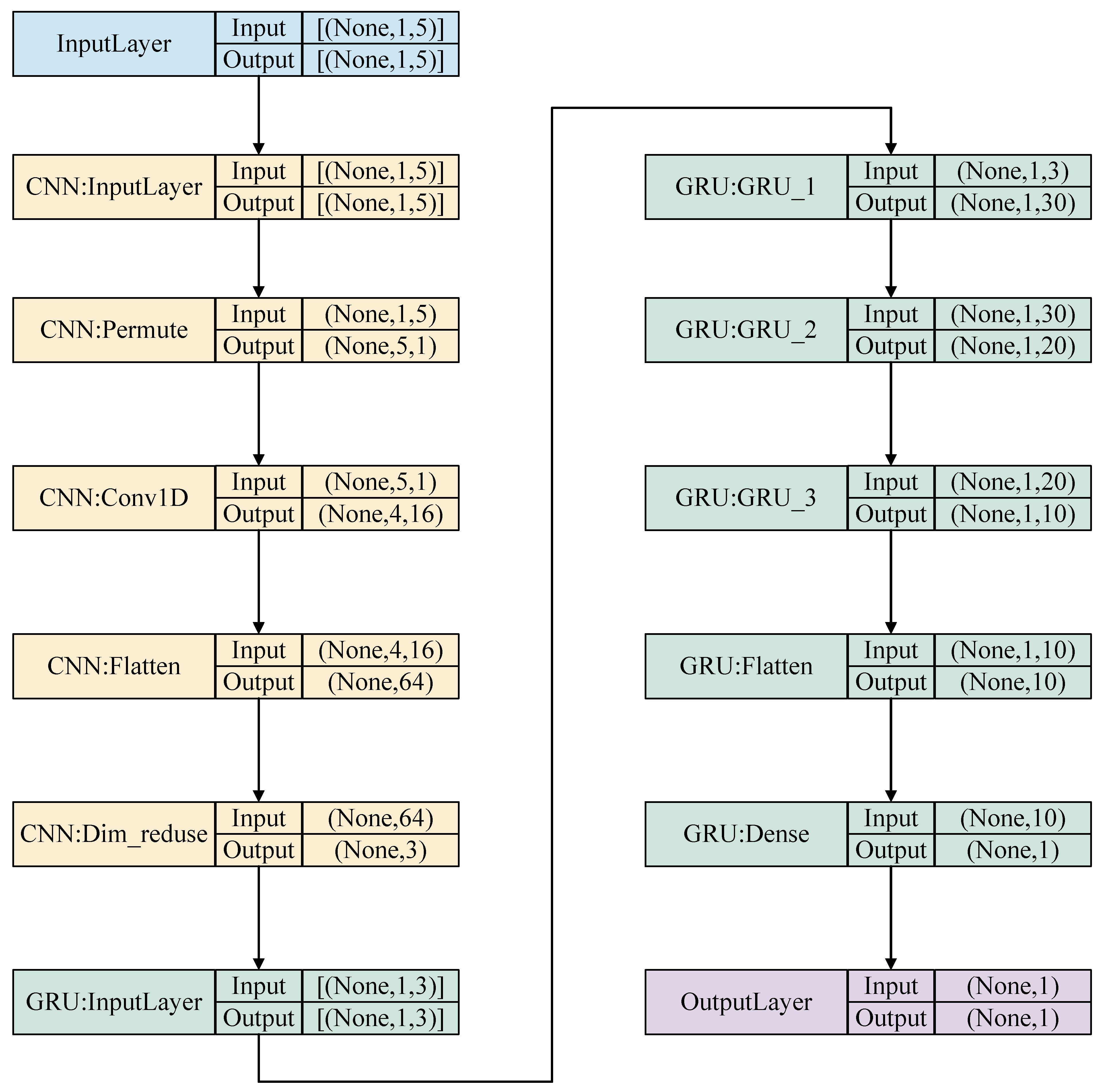
In this paper, the model is based on Python version 3.8.8 and the Keras deep-learning framework, and the model structure parameters were visualized using the Graphviz module, which is shown in Figure 18.
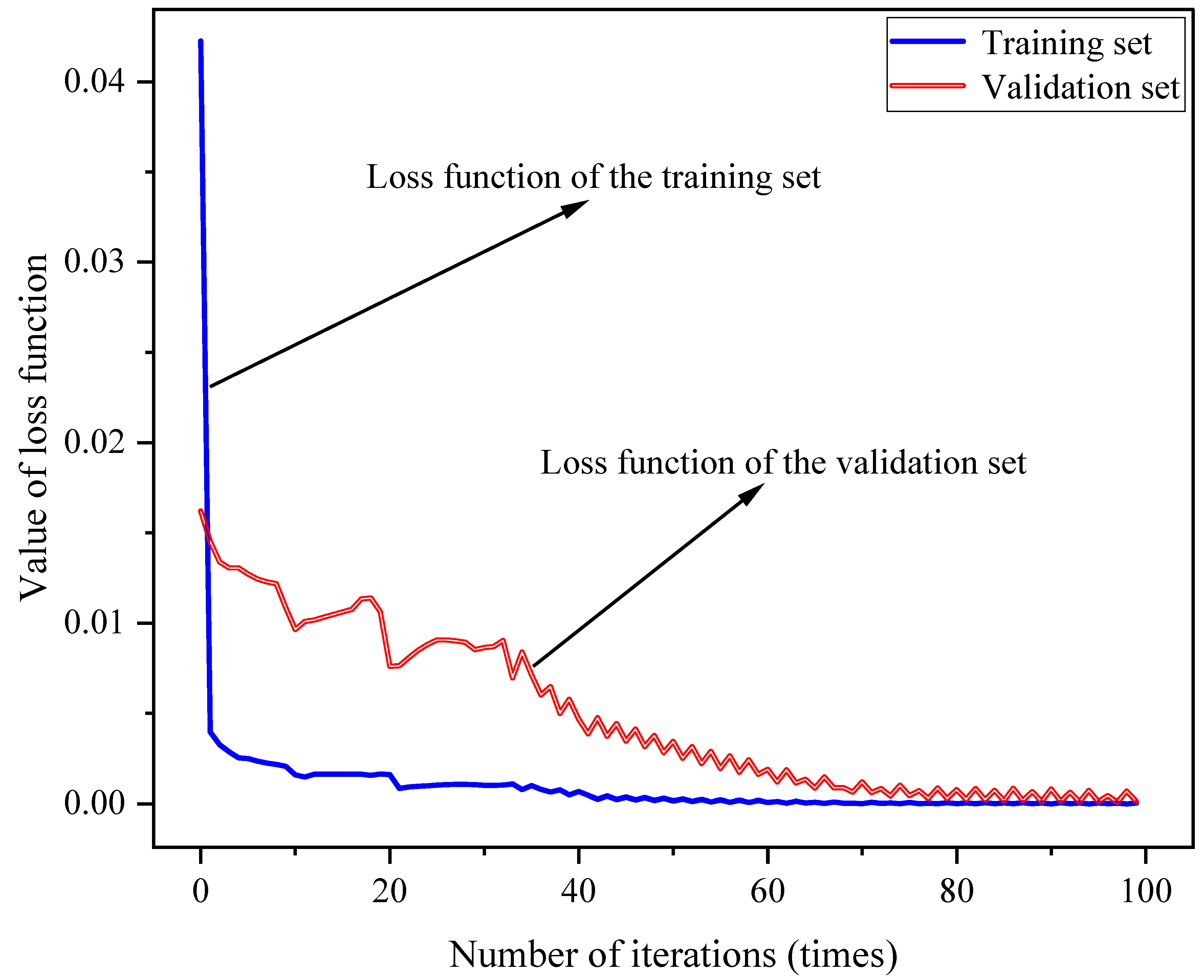
Considering that the failure of AC contactors mostly occurs at the end of service life in practice, the data set division was selected to be 70% as the training set, 20% as the validation set and 10% as the test set, sequentially. The loss-function curves of model training are shown in Figure 19.
When the number of iterations was lower than 80 times, the loss-function curves of the training set and the validation set show a decreasing trend. When the number of iterations reaches 80 times, the loss-function converges completely, after which the loss function of the validation set does not show a steep rising trend and is not overfitted, so the model training effect is good.

5.4. Comparison of Prediction Results

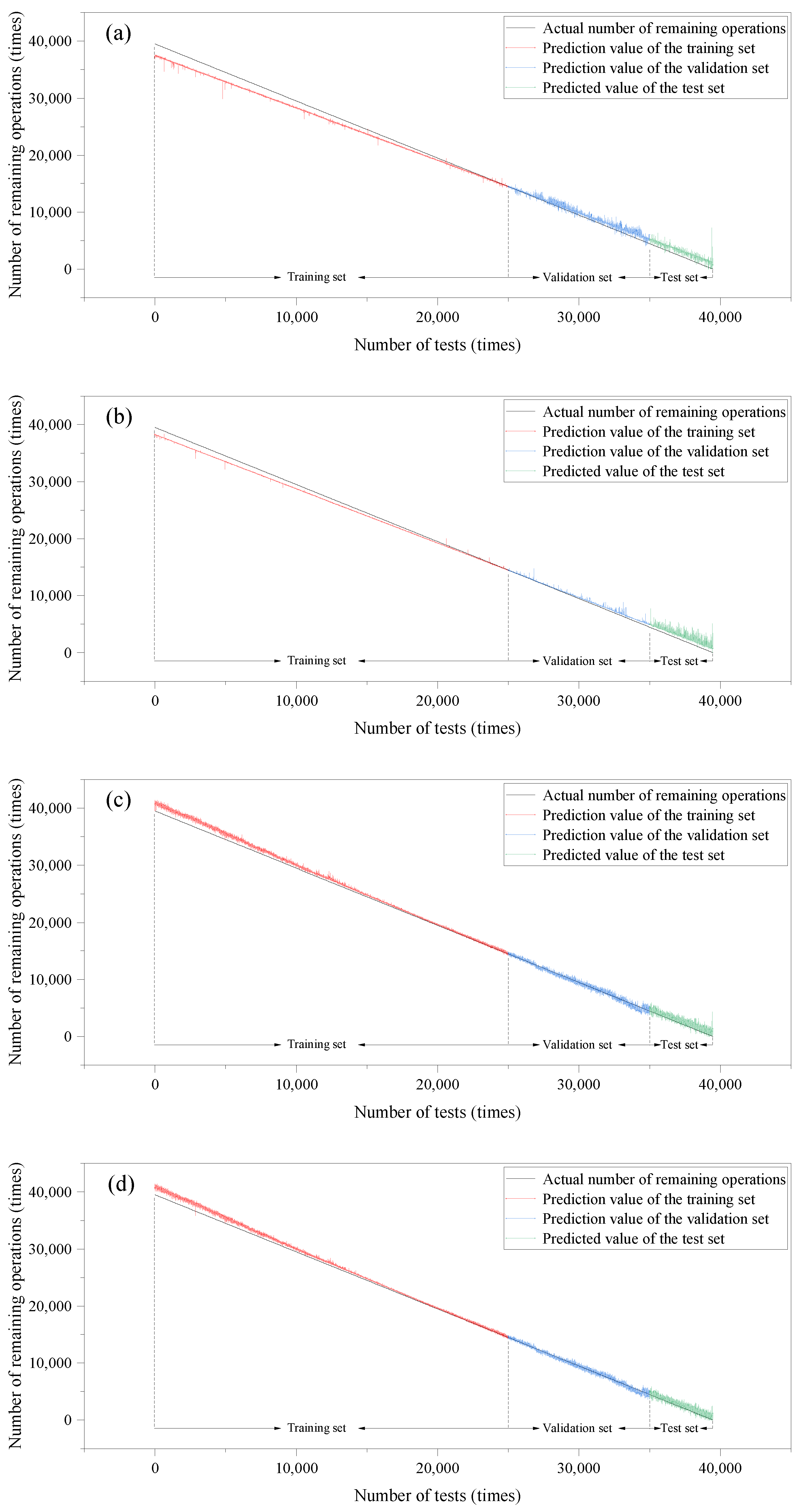
As shown in Figure 20 and Figure 21, in order to reflect the superiority of the proposed method, RNN, LSTM and GRU, which are popular in the field of timing prediction, were compared with the CNN-GRU method proposed in this paper before and after feature selection. The comparison shows that the remaining number of AC contactor openings predicted by the RNN, LSTM, GRU and CNN-GRU methods proposed in this paper are all very close to the actual number, but the curve of the prediction results based on the CNN-GRU method matches the curve of the actual life the best and has the smallest overall fluctuation. The quantitative analysis of all models before and after feature selection is shown in Table 5 and Table 6.
According to Table 5 and Table 6, it can be seen that the prediction of AC-contactor residual-electrical-endurance under the same model with feature selection is not only effective in terms of accuracy but also the significantly reduced the computation time compared to the model without feature selection. Both before and after feature selection, the prediction results of the CNN-GRU method compared with those of the RNN, LSTM, and GRU methods, the RMSE, MAE, maximum absolute error, and standard deviation of prediction accuracy are the smallest, which indicate that the CNN-GRU method has higher accuracy and stability. The R 2 is the highest, and the model is highly interpretable, while the model computation time is the shortest, and the overall advantage is obvious. The overall prediction accuracy of the CNN-GRU method after feature selection is significantly improved from 83.20% to 96.63% compared with the RNN method, where the RNN method is the worst among the temporal prediction models. The accuracy of the model using CNN-GRU method is significantly improved.
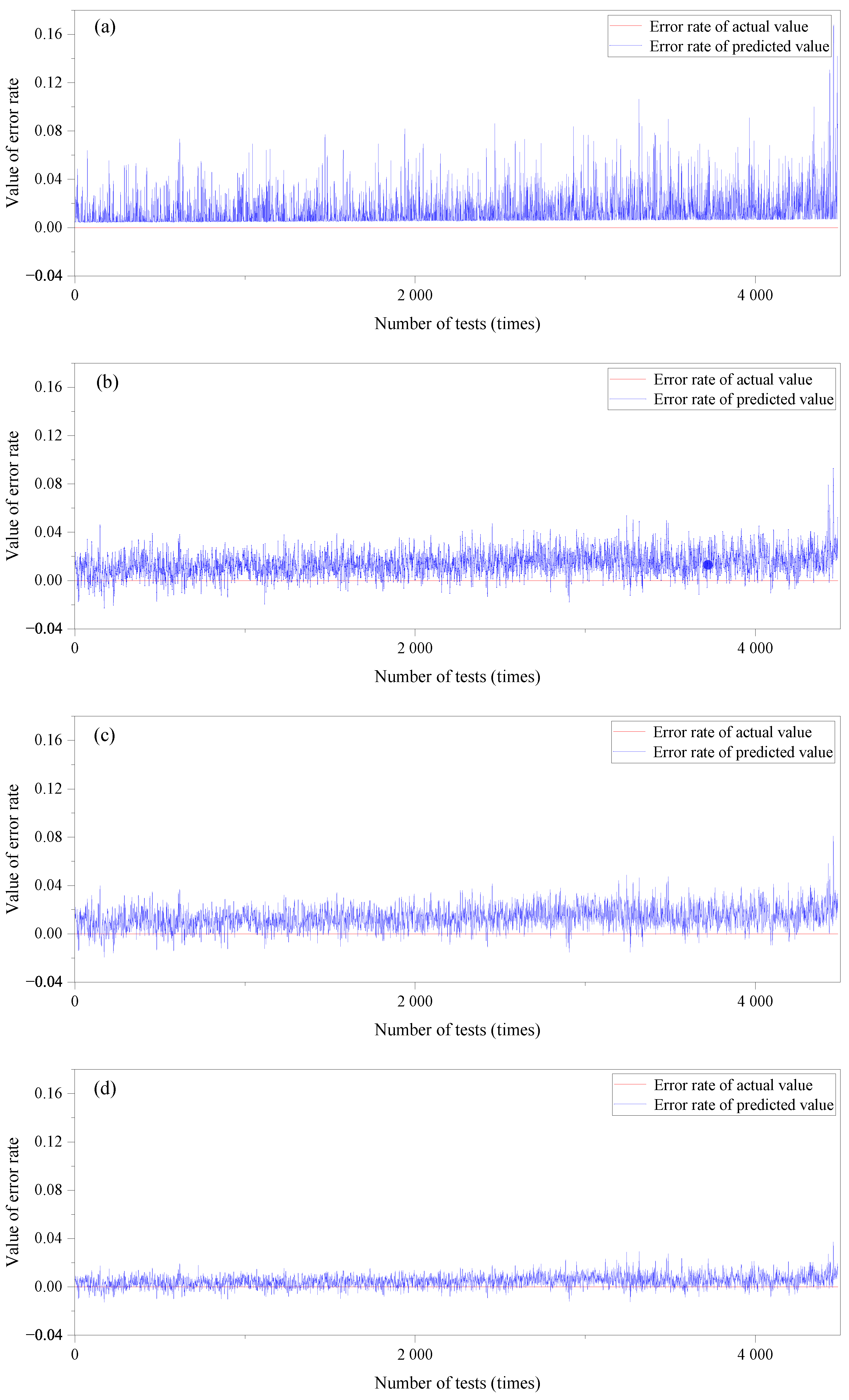
In order to compare the difference between different methods and more obviously reflect the superiority of the prediction method in this paper, the error rate of the prediction results of each methods’ test set after feature selection is compared and analyzed in this paper, and the comparison results of the error rate is shown in Figure 22.
The comparison results show that after feature selection, the error rate of the CNN-GRU method does not have a large deviation compared with the error rate of the RNN, LSTM and GRU prediction results, and the overall stability is the highest with high reliability. The test-set prediction results were also compared with some randomly selected results, and the sampling comparison results are shown in Figure 23.
It can be clearly seen from the comparison results that the results predicted in this paper are closest to the actual values and have the highest accuracy. In summary, the residual-electrical-endurance prediction model of an AC contactor based on the CNN-GRU method has high accuracy and robustness, which can meet the practical engineering needs and has wide application prospects.

6. Conclusions

This paper proposed a residual-electrical-endurance prediction model for AC contactors based on the CNN-GRU method and used the CJX2-8011 model AC contactor for verification and analysis. The conclusions are as follows.
(1) The feature parameters of the AC contactor were extracted through the full-life test platform; the importance of the feature parameters on the residual-electrical-endurance was calculated using NCA. The correlation analysis of the features was carried out using MIC. The optimal subset of features that effectively characterize the degradation state of the AC contactor was selected with consideration of both importance and correlation.
(2) The convolutional computation and pooling operation were used in CNN for feature vector extraction and dimensionality reduction and compression processing. The regular information between features was extracted deeply, further reducing the risk of model training overfitting.
(3) The concept of temporal degradation was introduced into the prediction of the residual-electrical-endurance of the AC contactor. The degradation process of the AC contactor is regarded as a long time sequence, and the information of the long-time history features was memorized by GRU with full consideration of the correlation of the previous and later states to achieve the temporally accurate prediction of the residual-electrical endurance of the AC contactor.
(4) A residual-electrical-endurance prediction model of AC contactors based on the CNN-GRU method was constructed. The case analysis shows that the prediction model has small error and high effective accuracy, which can solve the long-time-series prediction problem effectively. This method provides a new theorisation for the residual-electrical-endurance prediction problem of switchgear and electrical equipment.

Author Contributions

S.L. proposed the methodology, conducted project administration, and provided resources and funding acquisition. S.G. proposed the methodology, performed software operations and wrote the original draft. S.P. performed software operations and reviewed and edited the manuscript. Y.L. validated the algorithms. J.L. supervised the experiment. All authors have read and agreed to the published version of the manuscript.

Funding

This research was funded by Major Science and Technology Projects of Liaoning Province grant number 2020JH1/10100012, Project of Liaoning Provincial Department of Education grant number LJGD 2020001, and the Shenyang Young and Middle-aged Scientific and Technological Innovation Talents Program grant number RC210354. The APC was funded by Major Science and Technology Projects of Liaoning Province grant number 2020JH1/10100012.

Institutional Review Board Statement

Not applicable.

Informed Consent Statement

Not applicable.

Data Availability Statement

Not applicable.

Conflicts of Interest

The authors declare no conflict of interest.

References

  1. Liu, S.; Wang, Y.; Liu, Z.; Cao, Y.; Zhu, S. Condition evaluation of AC contactor based on the grey fuzzy theory. In Proceedings of the 2017 4th International Conference on Electric Power Equipment-Switching Technology (ICEPE-ST), Xi’an, China, 22–25 October 2017; pp. 238–242. [Google Scholar]
  2. Zhang, C.; Xu, Z. A Digital Controller for Series of AC Contactors. In Proceedings of the 2019 5th International Conference on Electric Power Equipment-Switching Technology (ICEPE-ST), Kitakyushu Japan, 13–16 October 2019; pp. 702–705. [Google Scholar]
  3. Yang, D.; Gao, X.; Ma, Z.; Cui, E.; Zhang, H. Novel voltage sag protection topology of contactors for uninterrupted switching capability. IEEE Trans. Ind. Appl. 2018, 54, 3170–3178. [Google Scholar] [CrossRef]
  4. Zong, M.; heng Li, Y. Researchon the key technology of contactor electrical life test. In Proceedings of the 2015 18th International Conference on Electrical Machines and Systems (ICEMS), Pattaya, Thailand, 25–28 October 2015; pp. 312–315. [Google Scholar]
  5. Wu, Z.; Wu, G.; Huang, H.; You, Y. A novel residual electrical endurance prediction method for low-voltage electromagnetic alternating current contactors. IEEE Trans. Components Packag. Manuf. Technol. 2015, 5, 465–473. [Google Scholar]
  6. Kumari, S.; Kumar-M, P.; Muralidhar, M. Reliability estimation of distribution components-Contactors. In Proceedings of the 2016 IEEE PES Asia-Pacific Power and Energy Engineering Conference (APPEEC), Xi’an, China, 25–28 October 2016; pp. 2066–2070. [Google Scholar]
  7. Wu, Z.; Wu, G.; Chen, C.; Fang, Y.; Pan, L.; Huang, H. A novel breaking strategy for electrical endurance extension of electromagnetic alternating current contactors. IEEE Trans. Compon. Packag. Manuf. Technol. 2016, 6, 749–756. [Google Scholar] [CrossRef]
  8. Zheng, S.; Niu, F.; Li, K.; Huang, S.; Liu, Z.; Wu, Y. Analysis of electrical life distribution characteristics of AC contactor based on performance degradation. IEEE Trans. Compon. Packag. Manuf. Technol. 2018, 8, 1604–1613. [Google Scholar] [CrossRef]
  9. Cui, H.; Wu, Z.; Wu, G.; Xu, X.; You, Y.; Fang, Y. Convolutional neural networks for electrical endurance prediction of alternating current contactors. IEEE Trans. Compon. Packag. Manuf. Technol. 2019, 9, 1785–1793. [Google Scholar] [CrossRef]
  10. Sun, S.; Wang, Q.; Du, T.; Wang, J.; Li, S.; Zong, J. Quantitative evaluation of electrical life of AC contactor based on initial characteristic parameters. IEEE Trans. Instrum. Meas. 2020, 70, 1–10. [Google Scholar] [CrossRef]
  11. Li, K.; Zhao, C.; Niu, F.; Zheng, S.; Duan, Y.; Huang, S.; Wu, Y. Electrical performance degradation model and residual electrical life prediction for AC contactor. IEEE Trans. Compon. Packag. Manuf. Technol. 2020, 10, 400–417. [Google Scholar] [CrossRef]
  12. Abirami, S.; Ruthvik, S.; Ali, M.S.; Kumar, R.S.; Kumar, J.S. AC Contactor Electrical Health Estimator Model. In Proceedings of the IOP Conference Series: Materials Science and Engineering; IOP Publishing: Bristol, UK, 2021; Volume 1145, p. 012070. [Google Scholar]
  13. Kumbhar, A.; Dhawale, P.G.; Kumbhar, S.; Patil, U.; Magdum, P. A comprehensive review: Machine learning and its application in integrated power system. Energy Rep. 2021, 7, 5467–5474. [Google Scholar] [CrossRef]
  14. Wang, S.; Jin, S.; Bai, D.; Fan, Y.; Shi, H.; Fernandez, C. A critical review of improved deep learning methods for the remaining useful life prediction of lithium-ion batteries. Energy Rep. 2021, 7, 5562–5574. [Google Scholar] [CrossRef]
  15. Yang, B.; Liu, R.; Zio, E. Remaining useful life prediction based on a double-convolutional neural network architecture. IEEE Trans. Ind. Electron. 2019, 66, 9521–9530. [Google Scholar] [CrossRef]
  16. Kido, S.; Hirano, Y.; Hashimoto, N. Detection and classification of lung abnormalities by use of convolutional neural network (CNN) and regions with CNN features (R-CNN). In Proceedings of the 2018 International Workshop on Advanced Image Technology (IWAIT), Chiang Mai, Thailand, 7–9 January 2018; pp. 1–4. [Google Scholar]
  17. Bedi, J.; Toshniwal, D. Empirical mode decomposition based deep learning for electricity demand forecasting. IEEE Access 2018, 6, 49144–49156. [Google Scholar] [CrossRef]
  18. Shen, C. A transdisciplinary review of deep learning research and its relevance for water resources scientists. Water Resour. Res. 2018, 54, 8558–8593. [Google Scholar] [CrossRef]
  19. Yang, S.; Yu, X.; Zhou, Y. Lstm and gru neural network performance comparison study: Taking yelp review dataset as an example. In Proceedings of the 2020 International Workshop on Electronic Communication and Artificial Intelligence (IWECAI), Shanghai, China, 12–14 June 2020; pp. 98–101. [Google Scholar]
  20. Que, Z.; Jin, X.; Xu, Z. Remaining useful life prediction for bearings based on a gated recurrent unit. IEEE Trans. Instrum. Meas. 2021, 70, 1–11. [Google Scholar] [CrossRef]
  21. Wei, M.; Gu, H.; Ye, M.; Wang, Q.; Xu, X.; Wu, C. Remaining useful life prediction of lithium-ion batteries based on Monte Carlo Dropout and gated recurrent unit. Energy Rep. 2021, 7, 2862–2871. [Google Scholar] [CrossRef]
  22. Roweis, S.; Hinton, G.; Salakhutdinov, R. Neighbourhood component analysis. Adv. Neural Inf. Process. Syst.(NIPS) 2004, 17, 4. [Google Scholar]
  23. Zhang, C.; Liu, L.; Zhang, S.; Huang, C. Microarray Data Classification Based on Neighbourhood Components Analysis Projection Method. In Proceedings of the 2021 IEEE 6th International Conference on Big Data Analytics (ICBDA), Xiamen, China, 5–8 March 2021; pp. 123–127. [Google Scholar]
  24. Reshef, D.N.; Reshef, Y.A.; Finucane, H.K.; Grossman, S.R.; McVean, G.; Turnbaugh, P.J.; Lander, E.S.; Mitzenmacher, M.; Sabeti, P.C. Detecting novel associations in large data sets. Science 2011, 334, 1518–1524. [Google Scholar] [CrossRef] [PubMed] [Green Version]
  25. Liang, T.; Zhang, Q.; Liu, X.; Lou, C.; Liu, X.; Wang, H. Time-frequency maximal information coefficient method and its application to functional corticomuscular coupling. IEEE Trans. Neural Syst. Rehabil. Eng. 2020, 28, 2515–2524. [Google Scholar] [CrossRef] [PubMed]
  26. Guo, X.; Zhao, Q.; Zheng, D.; Ning, Y.; Gao, Y. A short-term load forecasting model of multi-scale CNN-LSTM hybrid neural network considering the real-time electricity price. Energy Rep. 2020, 6, 1046–1053. [Google Scholar] [CrossRef]
  27. Zhai, N.; Yao, P.; Zhou, X. Multivariate Time Series Forecast in Industrial Process Based on XGBoost and GRU. In Proceedings of the 2020 IEEE 9th Joint International Information Technology and Artificial Intelligence Conference (ITAIC), Chongqing, China, 11–13 December 2020; Volume 9, pp. 1397–1400. [Google Scholar]
  28. Kingma, D.P.; Ba, J. Adam: A method for stochastic optimization. arXiv 2014, arXiv:1412.6980. [Google Scholar]
  29. GB14048.4-2020; Low-Voltage Switchgear and Control Equipment Part 4-1: Contactors and Motor Starters Electromechanical Contactors and Motor Starters. Standards Press of China: Beijing, China, 2011.
  30. Liu, Y.; Shuxin, L.; Cao, Y. Research on State Characterization of Switching Device Based on Modal Similarity Measurement. In Proceedings of the CSEE 2022, Lisbon, Portugal, 10–12 April 2022; pp. 173–176. [Google Scholar]
  31. Yang, Y.; Zhihong, X.; Fan, Y. An Indicator Reduction Method for Contactor’s Performance Evaluation. In Proceedings of the 2019 4th International Conference on Intelligent Green Building and Smart Grid (IGBSG), Yichang, China, 6–9 September 2019; pp. 173–176. [Google Scholar]
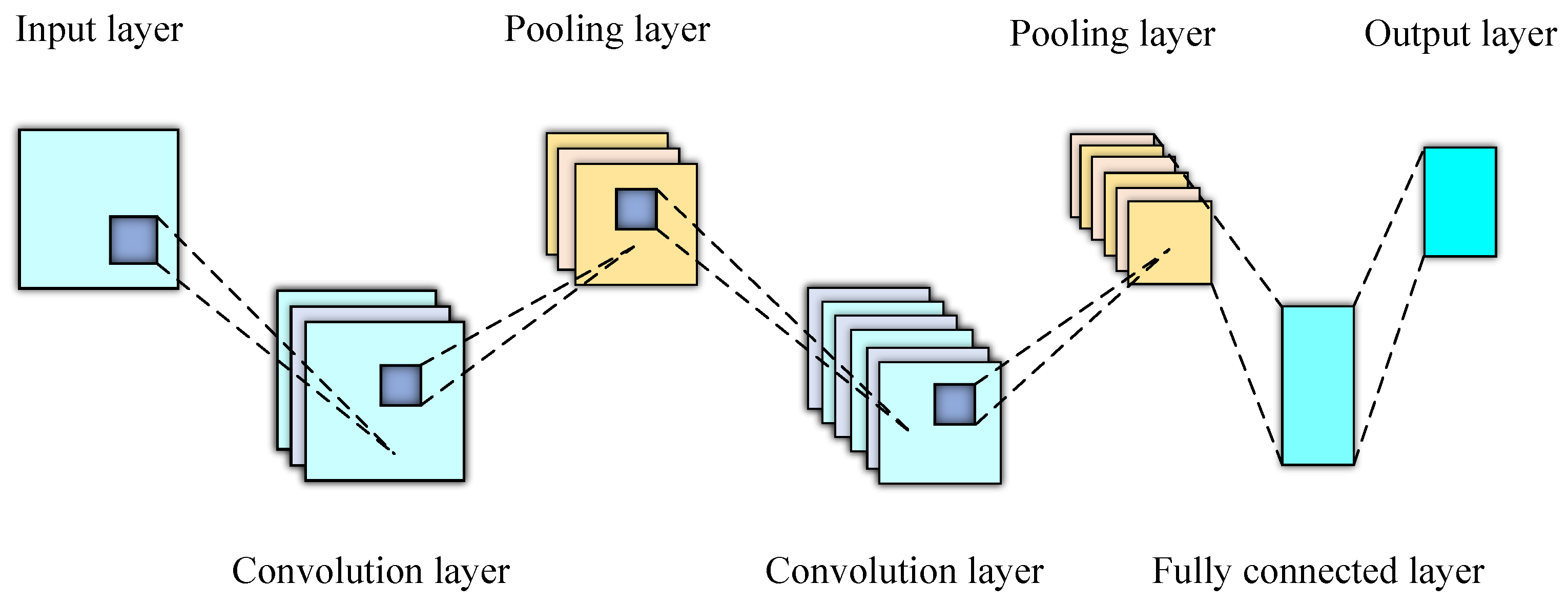
Figure 1. Structure diagram of CNN.
Machines 10 01067 g001
Figure 2. Internal structure diagram of GRU.
Machines 10 01067 g002
Figure 3. Circular structure of GRU.
Machines 10 01067 g003
Figure 4. Schematic diagram of the model structure.
Machines 10 01067 g004
Figure 5. Schematic diagram of the hardware circuit.
Machines 10 01067 g005
Figure 6. Electrical diagram.
Machines 10 01067 g006
Figure 7. Front-end control panel of the LabVIEW.
Machines 10 01067 g007
Figure 8. Program diagram of the LabVIEW.
Machines 10 01067 g008
Figure 9. Flow chart of software control.
Machines 10 01067 g009
Figure 10. Schematic diagram of the test platform.
Machines 10 01067 g010
Figure 11. Structure diagram of AC contactor.
Machines 10 01067 g011
Figure 12. The normal breaking and closing waveform.
Machines 10 01067 g012
Figure 13. Flow chart of case analysis.
Machines 10 01067 g013
Figure 14. Contrast diagram of contact ablation.
Machines 10 01067 g014
Figure 15. Diagram of feature trend change.
Machines 10 01067 g015
Figure 16. Comparison of NCA feature importance analysis.
Machines 10 01067 g016
Figure 17. Heat map of correlation coefficients.
Machines 10 01067 g017
Figure 18. Structural parameters of the model.
Machines 10 01067 g018
Figure 19. The loss-function curves.
Machines 10 01067 g019
Figure 20. Comparison of prediction results before feature selection. (a) RNN, (b) LSTM, (c) GRU, (d) CNN-GRU.
Machines 10 01067 g020
Figure 21. Comparison of prediction results after feature selection. (a) RNN, (b) LSTM, (c) GRU, (d) CNN-GRU.
Machines 10 01067 g021
Figure 22. Comparison of model errors. (a) RNN, (b) LSTM, (c) GRU, (d) CNN-GRU.
Machines 10 01067 g022
Figure 23. Sampling comparison diagram of prediction results.
Machines 10 01067 g023
Table 1. Test parameters of AC-4.
Test ConditionsAC-4
Load typeResistance load
Load voltage400 (380) V
Load current222 A
Coil voltage220 V
Power factor cos φ = 0.5
Connection conditions I / I e = 6 , U / U e = 1
Breaking conditions I c / I e = 6 , U r / U e = 1
Operation frequency 60   times / h
Sample frequency 1   M / Hz
Table 2. Technical parameters of the sensors.
LEM Sensor TypesLF310LV25-400
Sensor ParameterCurrentVoltage
Rated measurement value ± 300   A ± 400   A
Maximum measurement value ± 500   A ± 600   A
Rated working voltage ± 12   V ± 12   V
Measurement accuracy ± 0.2 % ± 0.8 %
Sensor linearity 0.05 % 0.2 %
Table 3. Status of Contacts.
TimeStatus
t a When the coil is energized, the electromagnetic attraction
force rises sharply, and the contacts act.
t b When the contacts are closed for the first time, a current is
generated between the contacts.
t c The contact is stably closed, the contact voltage is stable,
and the main circuit is connected.
t d The coil loses power, the electromagnetic attraction drops sharply,
and the contacts are separated.
t e The voltage between the contacts rises and arc generates.
t f The main circuit current crosses the zero point, and the arc is extinguished.
Table 4. Definition of feature parameters.
Serial NumberFeature NameComputational Formulas
1Contact resistance R j R j = 1 N j = 1 N u j 2 1 N j = 1 N i j 2 = j = 1 N u j 2 j = 1 N i j 2
2Pull-in time t x t x = t b t a
3Bounce time t t t t = t c t b
4Arcing time t arc t arc = t b t e
5Arc energy E E = j = e f u j · i j · Δ t = j = e f u j · i j f s
6Average arcing power P P = E Δ t · N = j = e f u j · i j N
7Release time t s t s = t e t d
Table 5. Model evaluation index before feature selection.
Prediction ModelsRNNLSTMGRUCNN-GRU
RMSE3468.523218.613020.182914.98
MAE1009.62736.12537.94432.34
R 2 0.36650.60650.75190.8310
Max Error7255.935107.344329.072489.70
Effective
precision
81.62%87.66%89.04%93.69%
Calculation time52.1 s49.6 s42.4 s35.6 s
Standard deviation of
prediction accuracy
1.2969%0.9761%1.0072%1.0466%
Table 6. Model evaluation metrics after feature selection.
Prediction ModelsRNNLSTMGRUCNN-GRU
RMSE3072.973066.953042.852742.03
MAE553.24582.54552.97225.16
R 2 0.63680.71940.75290.9538
Max Error6633.203662.673203.211474.50
Effective
precision
83.20%90.72%91.89%96.63%
Calculation time49.4 s45.9 s38.2 s31.8 s
Standard deviation of
prediction accuracy
1.3934%0.9994%0.9010%0.5006%
Publisher’s Note: MDPI stays neutral with regard to jurisdictional claims in published maps and institutional affiliations.