An Integrated Condition Monitoring Method for Rotating Machinery Based on Optimum Healthy State

Abstract

The degradation of a machine is nonlinear, which brings challenges to its performance assessment during condition monitoring, especially when there is a run-in period. Technically, the quantification of mechanical degradation is to define a distance metric from a health baseline. This paper develops an integrated condition monitoring scheme, where the degradation evaluation and fault diagnosis are combined by using one technical framework. Specifically, an optimum healthy state (OHS) is determined based on the clustering center of the self-organizing map (SOM) neural network instead of the commonly used initial working state. Then, the distance metric deviating from the OHS is defined as a health index, where the perceptual vibration hashing is improved to make it more sensitive to degradation. Visualized fault diagnosis is carried out by the SOM when the health index exceeds the preset threshold. Two cases with experiments are conducted to demonstrate the accuracy and robustness of the proposed method.

1. Introduction

It is a common phenomenon that a run-in period exists for a newly assembled machine to reach its best performance. The underlying mechanism [1] of the running in and its impact on the machine performance [2] draw the attention of researchers. However, the existence of running in also has a systematic influence on the condition-based maintenance of machines. Firstly, the mechanical degradation is not a simple downward curve; a health index should be sensitive to the changing of the machine condition, no matter it is getting better or getting worse. Secondly, it is a wrong convention to adopt the first sample acquired from a newly installed machine as the baseline for degradation assessment. Thirdly, condition monitoring should cover a machine’s whole life cycle, during which versatile decision-making support should be conducted, including running-in recognition, degradation assessment, fault diagnosis, etc.

Specifically, due to the run-in period, the degradation of a machine is not a linear process. Reflected on the vibration in the run-in period, the amplitude in the initial working state is slightly larger than that in the stable stage, which can be explained by certain undiscovered defects in the components [3], temperature influence or assembly accuracy. In other words, the machinery optimum healthy condition always appears after the device has been in operation for a while. Therefore, when utilizing distance metrics to quantify the machine health state, how the baseline should be defined is a problem to be solved. Meanwhile, much research has been focused on the practical application of condition-based maintenance in different aspects such as bearings [4,5], gears [6,7] and motors [8,9]. However, few studies focus on methods that carry out both degradation assessment and fault diagnosis under one technical framework, which results in lower efficiency of the condition monitoring during the practical operation.

A good quantification of the machine health condition is based on the effective features extracted from monitoring data. Basically, the extracted feature is a high information density form of the machine condition from the perspective of fault diagnostics and prognostics. Traditional statistical features in the time and frequency domain such as root mean square, kurtosis and crest factor are initially used for condition monitoring. Time–frequency feature extraction methods including short-time Fourier transform [10,11], wavelet-based methods [12,13] and empirical mode decomposition [14] are proposed, which perform well in uncovering more latent diagnosis information in nonstationary signals. More advanced features are further studied, such as Rényi entropy [15] and spectral kurtosis [16]. However, high data throughput during real-time condition monitoring can easily result in network congestion and heavy computing burden, which leads to a latency increase and efficiency decrease in condition monitoring. Perceptual vibration hashing, as an edge computing method, was developed by Liu et al. [17], which can extract and express the information on the machine condition while also reducing the data dimensionality by transforming the vibration signal into compact machine condition hashes (MCHs).

For the degradation assessment, a brand new machine is considered in a healthy state, deviating from which a health index is usually defined to quantify its degradation level. Numerous related studies have been conducted. Widodo et al. [18] proposed a health index by using principal components analysis (PCA) to reduce the feature dimensionality and calculating deviations between the unknown state and healthy state. Lei et al. [19] used a SOM to fuse mutual features and constructed a health index by calculating the distance deviating from its best matching unit (BMU) of the healthy state in the SOM. Dong et al. [20] used a deep autoencoder (DAE) to achieve feature extraction, expression and reduction. Then, the Mahalanobis distance was constructed as an index to evaluate the bearing health state. However, the baseline selection in distance metrics is usually determined based on experience. For example, samples obtained at the beginning of the operation are commonly set as the baseline. Based on the above analysis, it can be inferred that it is not the optimal choice. Therefore, it is needed to find a baseline selection method to obtain a sample which can represent the OHS of the machinery.

When there is an abnormality emerging from the distance metric, fault diagnosis should be carried out immediately to verify and recognize the malfunction for maintenance support. In recent years, intelligent fault diagnosis methods have been extensively researched, which can not only efficiently analyze enormous volumes of data but also automatically present the diagnosis results. Xue et al. [21] developed a fault diagnosis method for rotating machinery, where a deep convolution neural network is utilized for feature extraction and a support vector machine classifier is used for fault identification. Dhiman et al. [22] proposed an anomaly detection method for wind turbine gearboxes based on an adaptive threshold and twin support vector machine which shows excellent performance. The neural network is widely used for intelligent fault diagnosis because of its strong generalization ability. A SOM is a kind of unsupervised neural network proposed by Kohonen [23]. Based on the Mahalanobis–Taguchi system (MTS) and SOM, Hu et al. [24] developed a dynamic observer for bearing degradation evolution, which is called the MTS–SOM system. The experiment results showed an excellent visualization ability of the SOM on fault evolution trajectory tracking. Saucedo-Dorantes et al. [25] proposed a fault diagnosis method for an electric machine based on a hierarchical SOM, which exhibits a good fault classification performance.

Based on the above analysis, an integrated condition monitoring scheme for rotating machinery is introduced in this paper. The major novelties and contributions of this paper can be summarized in four aspects:

(1)

In this proposed integrated condition monitoring method, both degradation evaluation and visualized fault identification are carried out under one technical framework.

(2)

For degradation evaluation, an OHS selection method is proposed based on the clustering center of the SOM neural network instead of the initial working state. Then, the distance metric deviating from the OHS is set as the health index.

(3)

Based on the original perceptual vibration hashing algorithm, an improved perceptual vibration hashing is proposed to make it more sensitive to partial differences during condition monitoring.

(4)

Two case studies are conducted. The proposed framework is first verified by the public bearing run-to-failure dataset. Then, a practical rotary torsional fatigue test is further carried out to validate the accuracy and robustness of the proposed scheme.

The composition of this paper is as follows. In Section 2, the theoretical foundation of the improved perceptual vibration hashing (IPVH) and SOM neural network is introduced in detail. In Section 3, the proposed integrated condition monitoring method is presented and a detailed description of degradation evaluation and fault identification is given. In Section 4, two cases with experiments are analyzed to illustrate the application results of the proposed methods. After it, in Section 5, the conclusions of the paper are given.

2. Preliminaries

2.1. Improved Perceptual Vibration Hashing

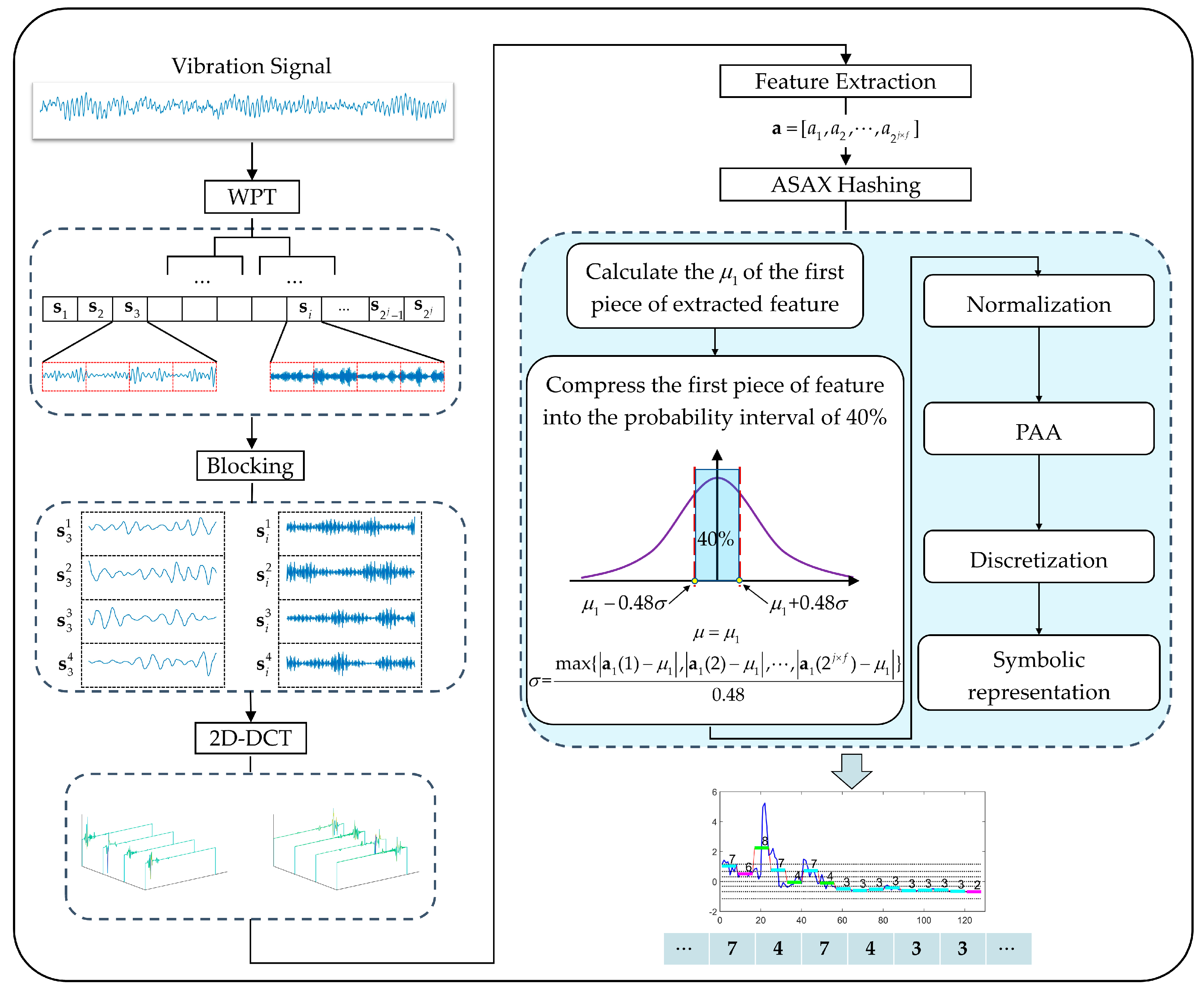
The perceptual vibration hashing proposed by Liu et al. [17] is an edge computing method that extracts health information from raw vibration signals and represents it with compact machine condition hashes (MCHs). However, a naive implementation of the perceptual vibration hashing approach may result in MCHs with a high degree of similarity even when dealing with input signals with partially significant amplitude differences. As a result, the distance metric between the corresponding MCHs remains small. Therefore, an IPVH is proposed in this research with more emphasis on partial differences. Compared with the original perceptual vibration hashing algorithm, a detailed description of the improved part of the algorithm can be found in the following Step 5, which is also highlighted in the blue area as illustrated in Figure 1. The process of the IPVH is shown below:

Step 1: a raw vibration signal $s$ is divided into $2^j$ frequency bands $s_1,s_2,\cdots ,s_{{}^{2^j}}$ by the j-level wavelet packet transform (WPT).

Step 2: one sub-band signal $s_i$ is sliced up into f blocks. For instance, a 1024-point reconstructed coefficient $s_i$ can be divided into four blocks to obtain a matrix $s_i=[s_i^1;s_i^2;s_i^3;s_i^4]$.

Step 3: A two-dimensional discrete cosine transform (2D-DCT) is implemented on every block. As a result, a coefficient matrix $f_i=[f_i^1;f_i^2;f_i^3;f_i^4]$ can be obtained.

Step 4: the feature is extracted from each $f_i$ to obtain a feature vector and is cascaded to obtain a sub-band feature vector $a=[a_1,a_2,\cdots ,a_{2^{j\times f}}]$ for $s$.

Step 5: hashing with the improved Adaptive Symbolic Aggregate Approximation (ASAX):

For most families of normalized time series, Gaussian distribution is assumed in their values. In this part, parameters of an unknown Gaussian distribution are estimated to make it possible that the sub-band features collected in the healthy state can only be compressed and mapped into a probability interval of 40%.

Figure 1. Flow chart of the proposed IPVH.

Figure 1. Flow chart of the proposed IPVH.

Firstly, calculate the mean value ${\mu }_1$ of the first sub-band feature $a_1$ during condition monitoring. For any Gaussian distribution, the probability $\mathrm{P}(\mu -t\sigma \le x\le \mu +t\sigma )$ only depends on the value of parameter t, which has nothing to do with the mean value $\mu$ and standard deviation $\sigma$. By looking up the normal distribution table, it can be known that $\mathrm{P}(\mu -0.48\sigma \le x\le \mu +0.48\sigma )\approx 40\%$. So, set

$$\max \{\left|a_1\left(1\right)-{\mu }_1\right|,\left|a_1\left(2\right)-{\mu }_1\right|,\cdots ,>|a_1{(2}^{j\times f})-{\mu }_1|\}=0.48\sigma$$

(1)

Then, the parameters of the Gaussian distribution can be estimated, which are shown in Equations (2) and (3):

$$\mu ={\mu }_1$$

(2)

$$\sigma =\frac{\max \{\left|a_1\left(1\right)-{\mu }_1\right|,\left|a_1\left(2\right)-{\mu }_1\right|,\cdots ,|a_1{(2}^{j\times f})-{\mu }_1|\}}{0.48}$$

(3)

Thirdly, normalize the sub-band features using the estimated $\mu$ and $\sigma$, and reduce their dimension via piecewise aggregate approximation (PAA) [26]. Fourthly, an equiprobability theory is used for discretization [27]. The distribution space under the Gaussian curve is divided into k equal probability intervals. Finally, symbolic representation. A number size of k is utilized to describe the equal probability intervals so that any PAA coefficients located in any interval can be represented by a number.

By using the ASAX, a piece of compact MCH p can be obtained. Given two pieces of MCHs $p_1$ and $p_2$, the differences between the MCHs can be quantified by defining low-bounding distance functions in feature space as illustrated in Equation (4), where the m and z are the dimensions of the sub-band feature a and MCH p. Their lower bounding approximation to the Euclidean distance can be obtained by accumulating the piecewise distances. For example, when the Gaussian distribution space is divided into four equal probability intervals (k = 4), it means four numbers (1, 2, 3, 4) are used for symbolic representation. If $p_1^1=1$ and $p_2^1=3$, according to the look-up table in

Table 1. An illustration of the look-up table for dist() function.

	1	2	3	4
1	0	0	0.67	1.34
2	0	0	0	0.67
3	0.67	0	0	0
4	1.34	0.67	0	0

, the dist(1,3) is 0.67.

$$\mathrm{Distance}=\sqrt{\frac{m}{z}}\sqrt{{\displaystyle \sum _{i=1}^z{(dist(p_1^i,p_2^i))}^2}}$$

(4)

In the end, a piece of the 1024-point raw signal is converted into a piece of MCH with several numbers. It can achieve not only a comprehensive representation of raw vibration signals but also more storage resources saving.

2.2. Self-Organizing Maps Neural Network

An SOM is an adaptive unsupervised neural network suitable for data clustering and was proposed by Kohonen. The basic idea of the algorithm is considered a nonlinear transformation from the input feature with high dimensionality to an output space with low dimensionality. It has two layers including an input layer and a competitive layer. The competitive layer consists of a two-dimensional array of neurons which are interconnected with each other. Each neuron can be represented by a weight vector $w$.

By using an SOM, all the input vectors can be clustered in groups based on the distance. The unified distance matrix (U-matrix) can reflect the distance between neurons, which provides visualization of the whole cluster structure of the SOM. Through neurons which are labeled by various types of colors or letters, different clusters can be identified.

3. Proposed Framework of the Integrated Condition Monitoring Method

As shown in Figure 2, under the same technical framework, both degradation evaluation and visualized fault identification are carried out. In a condition monitoring scenario, raw vibration signals are constantly collected and transformed into MCHs through the IPVH algorithm. With the advance of the condition monitoring process, an optimum health state (OHS) is determined according to the clustering characteristics of the monitored data. Then, a health index is defined as the distance metric deviating from the OHS value. The visualized fault diagnosis will be triggered when the health index exceeds the threshold. The detailed description is illustrated in Section 3.1 and Section 3.2.

3.1. Degradation Assessment Based on OHS

In order to obtain an OHS sample as the health baseline, an OHS selection method based on the SOM is proposed.

Step 1: initialize four empty matrixes $B_1=B_2=B_3=D=[]$

Step 2: During the condition monitoring, the sets $B_1$ and $B_2$ keep collecting sub-band feature $a_i$ and MCH $p_i$ in Section 2.1. In this research, all $a_i$ is 128-dimensional and $p_i$ is 32-dimensional.

Step 3: As shown in Equation (5), when the quantity of samples in $B_1$ and $B_2$ equals the preset $\theta$, add all samples in $B_2$ to $D$. The parameter $\theta$ can be set based on the estimated operation time of the machine.

$$\begin{array}{l}{B}_1=[a_1,a_2,\cdots ,a_{\theta }]\\ B_2=[p_1,p_2,\cdots ,p_{\theta }]\end{array}$$

(5)

Step 4: Update the sample subscripts in $D=[p_1,p_2,\cdots ,p_{\beta }]$ in times sequence and put all samples in $D$ into the SOM network for clustering. By Equation (6), the mean distance $d_i$ from the neuron i to all other neurons is calculated, where the $w_i$ and $w_j$ are weight vectors of the neuron i and j. The n is the total quantity of neurons in the competitive layer of the SOM network. Then, as shown in Equation (7), a position function is defined to output the subscript c of the minimum value in $[d_1,d_2,\cdots ,d_n]$. The neuron c with the weight vector $w_c$ is considered the center neuron.

$$d_i=\frac{{\displaystyle {\displaystyle \sum }_{j=1}^n\parallel w_i-w_j{\parallel }_2}}{n},i=1,2,\cdots n$$

(6)

$$c=\mathrm{position}(\min ([d_1,d_2,\cdots ,d_n]))$$

(7)

Step 5: Calculate the distance $e_q$ between the MCH $p_q$ and center neuron c as illustrated in Equation (8). Then, through the position function, the subscript of the minimum value in $[e_1,e_2,\cdots ,e_{\beta }]$ is outputted as OHS. The MCH $p_{OHS}$ is considered to represent the machine OHS.

$$e_q=\parallel w_c-p_q{\parallel }_2,q=1,2,\cdots \beta$$

(8)

$$OHS=\mathrm{position}(\min ([e_1,e_2,\cdots ,e_{\beta }]))$$

(9)

Step 6: The OHS sample may need to be updated with the monitored data volume rising with time because the length of the run-in period varies from parts. To avoid endless updates, a trigger mechanism is designed. For all samples in $B_1$, as shown in Equation (10), an RMS is calculated and added to the $B_3$. Then, we initialize the $B_1=B_2=[]$.

$$r=\sqrt{\frac{{\displaystyle {\displaystyle \sum }_{i=1}^{\theta }{({\left|a_i\right|}^2)}^2}}{\theta }}$$

(10)

Step 7: Repeat step 2 to step 6. When the latest two changing rates of RMS in $B_3$ is lower than a preset threshold l for two times, as shown in Equation (11), the $p_{OHS}$ will not be updated. The o is the size of $B_3$, which increases by 1 every time the step 2 to step 6 are completed.

$$\frac{r_o}{r_{o-1}}<l \mathrm{and} \frac{r_{o-1}}{r_{o-2}}<l,o\ge 3$$

(11)

After the OHS sample $p_{OHS}=[p_{OHS}^1,p_{OHS}^2,\cdots ,p_{OHS}^{32}]$ is determined, we are given any piece of MCH $p=[p^1,p^2,\cdots ,p^{32}]$. As shown in Equation (12), the distance metric deviating from the OHS is defined as the health index.

$$\mathrm{HI}=\sqrt{\frac{m}{z}}\sqrt{{\displaystyle {\displaystyle \sum }_{i=1}^z{(dist(p_{OHS}^i,p^i))}^2}}$$

(12)

During a condition monitoring scenario, the health index curve can be calculated in real time, with which the degradation trend can be clearly monitored. For the calculation of the degradation threshold, it is also based on the OHS. v points in the distance curve that are closest to the OHS are selected instead of the points obtained in the initial working state. Then, the degradation threshold can be determined by using the $\mu +4\sigma$ method [28] on the selected v points. When the degradation threshold is exceeded, the visualized fault diagnosis is triggered.

3.2. Visualized Fault Diagnosis Method Based on SOM

As illustrated in Figure 2, besides the use for the OHS sample selection, an SOM is also used for visualized fault diagnosis, which makes the developed method more integrative than other ordinary data-driven fault diagnosis using an SOM. In a specific condition monitoring application, before the different deteriorative machine conditions appear, the SOM is used to identify the optimum health condition, but with more MCHs under different machine conditions accumulated, a diagnostic SOM model can be established. Furthermore, the capability of the diagnostic SOM can also be updated with the continuously emerging new machine conditions. Finally, the machine condition can be recognized by the diagnostic SOM neural network automatically, with which the neurons with labels indicate machine conditions and the U-matrix can be used as an auxiliary method to estimate the fault type of data that is not located in the labeled neurons.

4. Experiments

To validate the reliability and efficiency of the proposed scheme, the XJTU-SY dataset [29] was used to demonstrate its theoretical viability. Its adaptability was verified through a practical rotary torsional fatigue test.

4.1. Case 1: XJTU-SY Dataset

4.1.1. Data Description of XJTU-SY Dataset

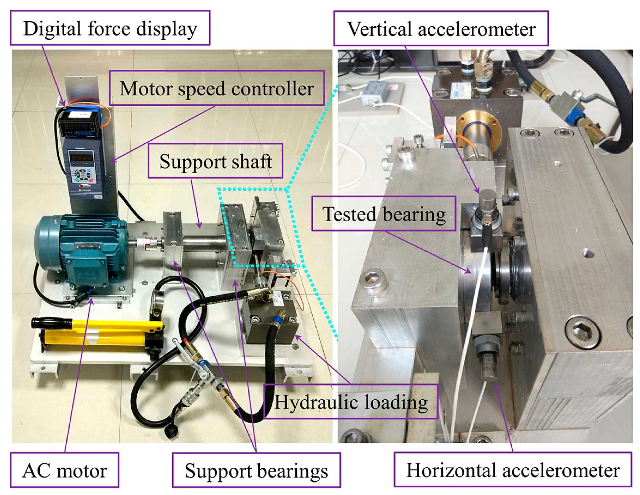
The overview of the test bench used to generate the XJTU-SY dataset is shown in Figure 3.

Table 2. Description of the XJTU-SY dataset.

Bearing Type	Working Condition	Dataset	File Count	Fault Type	Practical Life
LDK UER204	Radial force: 12 kN Rotating speed: 2100 r/min	Bearing 1_1	123	Outer race fault	2 h 3 min
		Bearing 1_2	161		2 h 41 min
		Bearing 1_3	158		2 h 38 min
		Bearing 1_4	122	Cage fault	2 h 2 min
		Bearing 1_5	52	Mixed fault	52 min

shows the datasets chosen in this paper. The tested bearings were LDK UER204. Five run-to-failure tests were conducted under the working condition of a rotating speed at 2100 r/min and radial force of 12 kN. It contained three types of bearing faults including an outer race fault (Bearing 1_1, Bearing 1_2, Bearing 1_3), cage fault (Bearing 1_4) and mixed fault (Bearing 1_5, outer race fault and inner race fault). The data sampling rate was 25.6 kHz. A piece of 1.28-s vibration data (32,768 datapoints) was collected every 1 min. Because of that, the load was applied in a horizontal direction, and the vibration signals obtained in this direction were used.

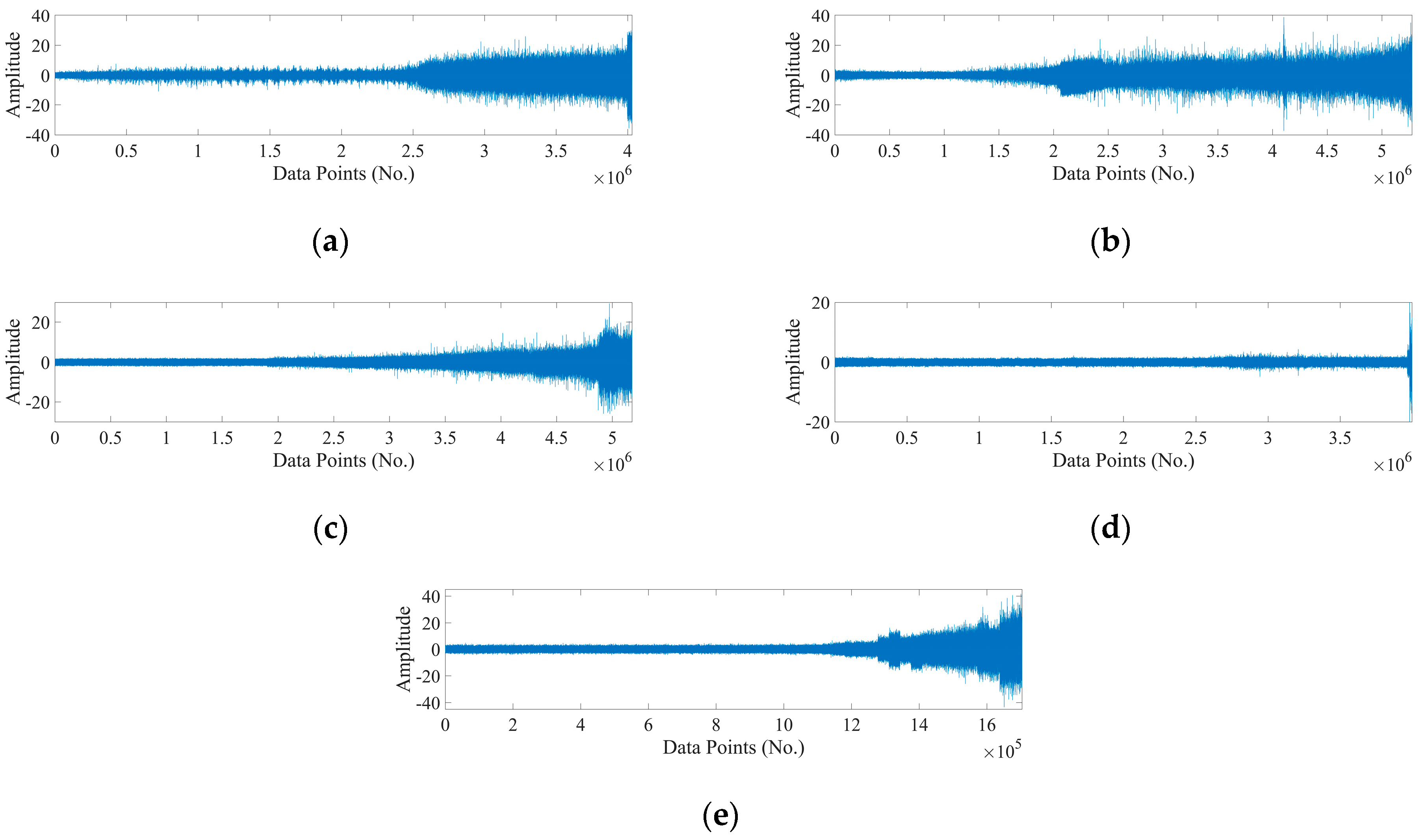
The whole vibration signals of the five run-to-failure tests are plotted in Figure 4. The signal amplitude in a healthy state was generally stable with random fluctuations. A slight decrease in amplitude from the start can be observed in Figure 4b of Bearing1_2, which denotes a clear existence of a run-in period. The increase in vibration amplitude means the degradation of bearings. As shown in Figure 4, most of the tested bearings had a clear and long degradation time, except for Bearing1_4. A slight increase could be observed from the vibration signals of Bearing 1_4, followed with a dramatic increase. It is also common in practical engineering that a weak damage leads to abrupt failure.

4.1.2. Degradation Assessment Based on an OHS

The IPVH method introduced in Section 2.1 was utilized to convert the vibration signals into MCHs. Specifically, 32 sub-bands were initially obtained by processing each 1024-point raw signal through a 5-level WPT. Each sub-band was cut into four blocks for 2D-DCT and feature extraction. After that, a 128-dimensional feature was obtained. By calculating the mean value of every 10 pieces of sub-band features, as presented in Figure 5, an average sub-band feature was displayed in a feature evaluation map. Then, each sub-band feature was transformed into MCHs with the ASAX with a 32-segment PAA and 80-size symbolic approximation. Finally, a 32-dimensional MCH was obtained from each feature.

As mentioned in Section 3.1, a trigger mechanism was used to determine when the update of the OHS should have been stopped. In this part, the $\theta$ was set as 10, which means the OHS was updated with every 10 new samples collected. The threshold for the changing rates of RMS $\gamma$ was set as 4%. When the selection of the OHS was finished, as shown in Figure 6, the changing rates of RMS during the whole process were illustrated. Through the method in Section 3.1, as shown in

Table 3. Results of OHS selection.

Dataset	Total Quantity of Samples	Quantity of Samples Put into the SOM Network (NO.)	Sample Located in the Clustering Center of SOM Network
Bearing 1_1	393	130	59th
Bearing 1_2	515	70	30th
Bearing 1_3	505	30	18th
Bearing 1_4	390	50	22nd
Bearing 1_5	166	40	17th

, the MCHs put into the SOM network were clustered and the MCH located in the clustering center of the SOM network was obtained as the baseline for degradation quantification.

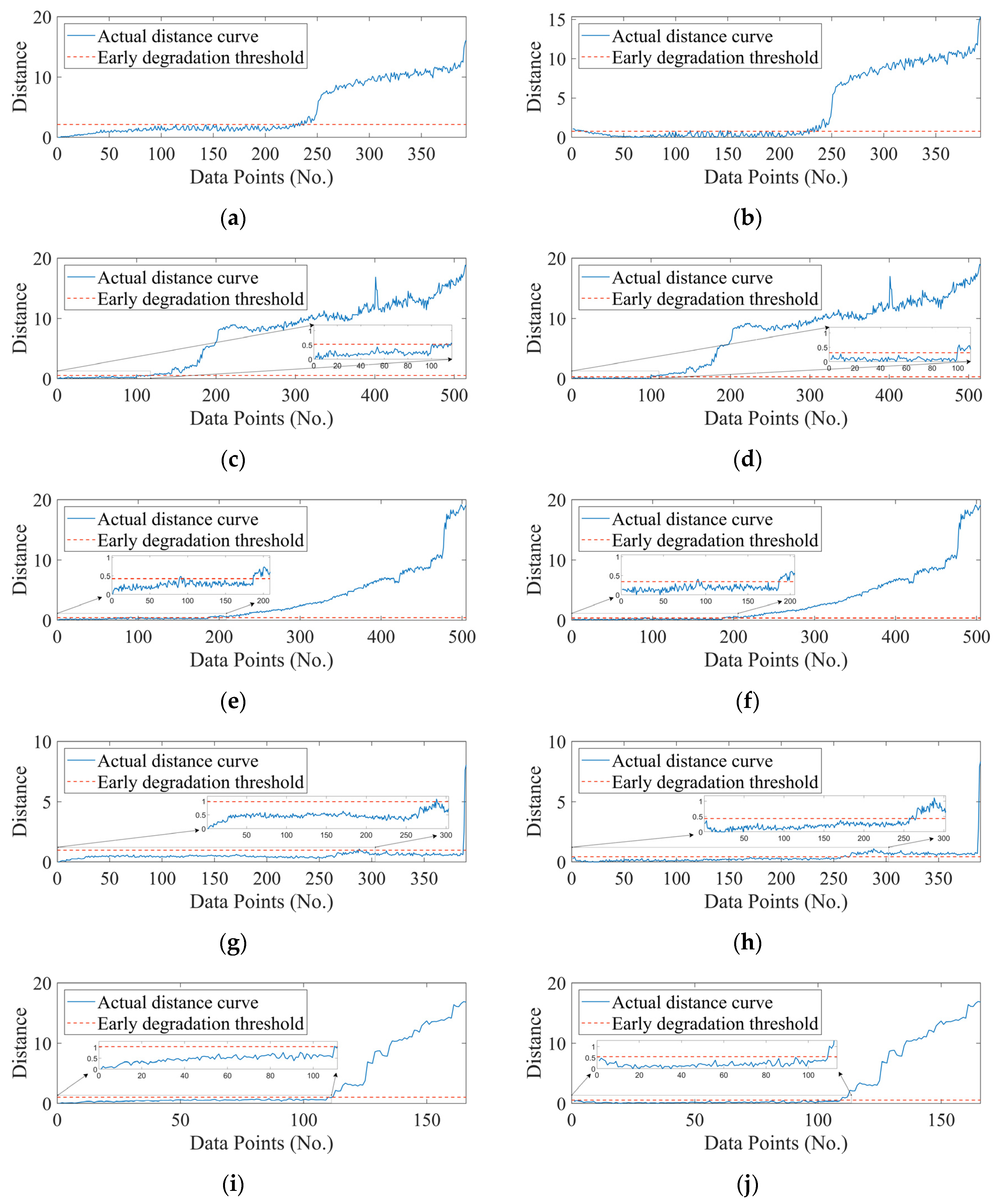
The distance metric can be calculated as the health index once the baseline has been established. Figure 7 compares the distance curves based on the first MCH with the ones based on the OHS.

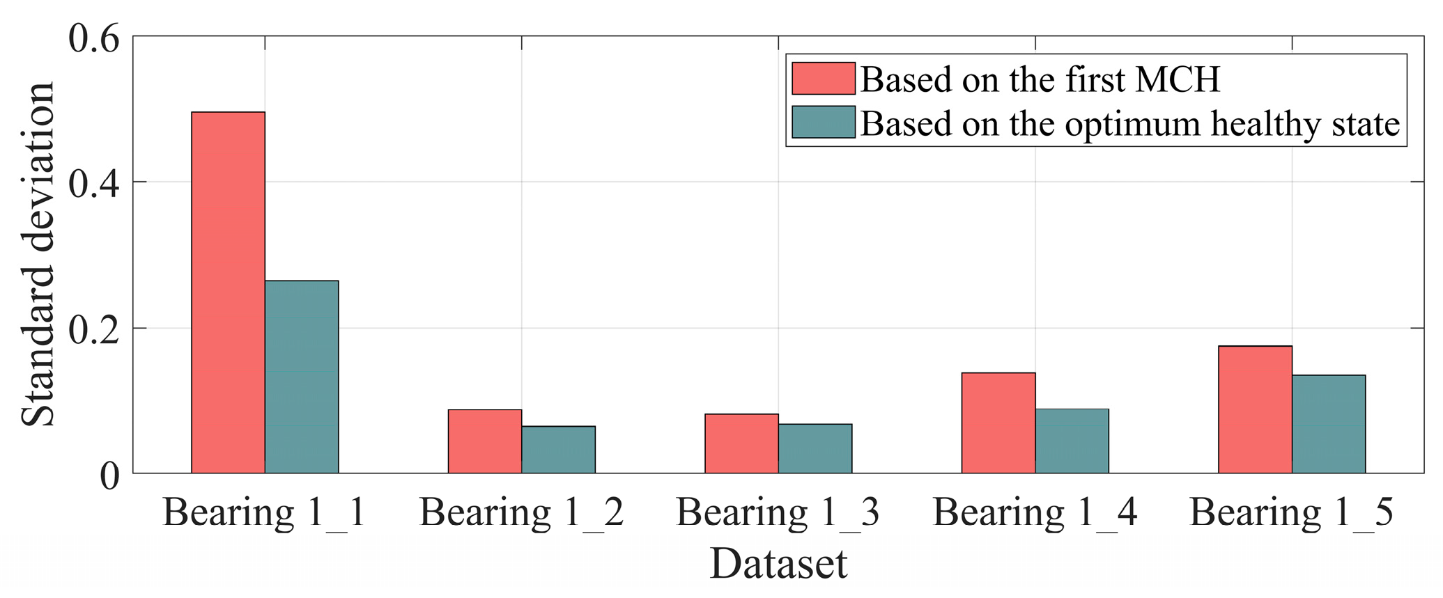
As shown in Figure 7, the change in the machine condition was much clearer and reasonable in the health index curve based on the OHS. First, earlier degradation could be more clearly detected in the distance curves based on the OHS. Comparative early degradation detection results are shown in

Table 4. Quantitative comparison of early degradation detection.

Dataset	Early Degradation Detection
	Distance Based on OHS	Distance Based on the First Sample	RMS	Pk-Pk	Crest Factor	Kurtosis
Bearing 1_1	227	227	227	232	Null	Null
Bearing 1_2	100	101	116	141	Null	Null
Bearing 1_3	187	187	187	187	199	193
Bearing 1_4	257	288	268	267	255	257
Bearing 1_5	110	110	104	107	Null	124

. Second, the distance curves based on the OHS were more stable before degradation occurred. As shown in Figure 8, the standard deviation of the distance in a healthy stage based on the OHS was smaller, which means the curve fluctuation was smaller. Thirdly, the developing trend of the distance curve denoted the machine condition more reasonably. To be more specific, the curve downtrend at the beginning better illustrated the run-in period of the tested bearings, which could be noticed in Figure 7b of Bearing 1_1 and Figure 7j of Bearing 1_5. During the healthy state, the distance metric remained within a narrower range so as to give prominence to the curve change, i.e., the machine condition change detection was more sensitive. For instance, the distance curves with the first sample as a health baseline in Figure 7c,g kept a generally increasing trend, which made the weak change inconspicuous. However, the corresponding curves based on the OHS could evidently present these changes for decision-making support.

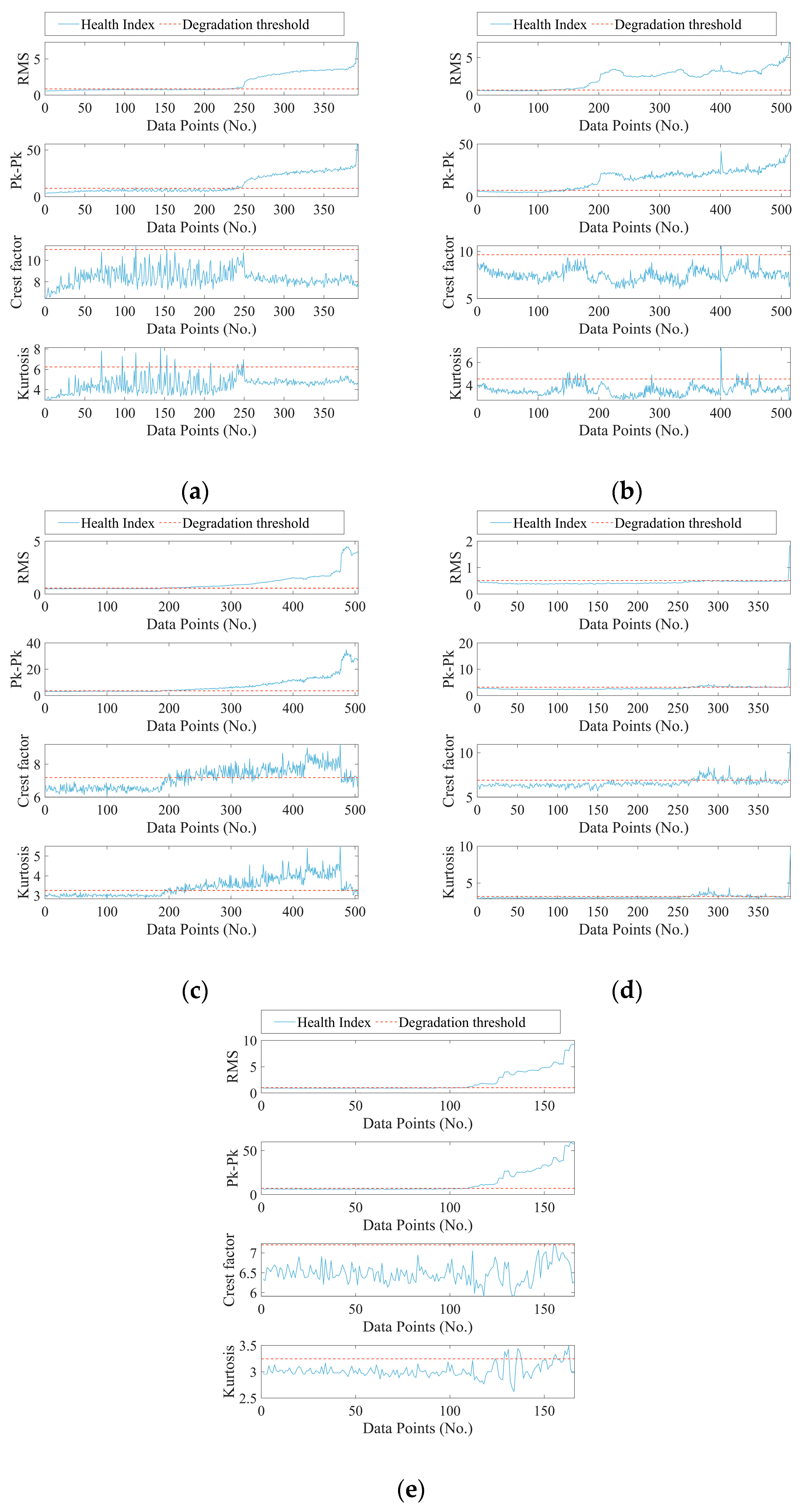
Moreover, the proposed method was compared with an RMS, peak-to-peak value, crest factor and kurtosis, which are commonly used health indexes in condition-based maintenance. As shown in Figure 9, the early degradation assessment results are illustrated with thresholding. Additionally, a quantitative comparison result is given in Table 4, where the number indicates the first datapoint exceeding the preset threshold and “Null” means no meaningful early failure detection. Compared with the distance curve based on the OHS, the method of the RMS and peak-to-peak value could achieve a similar effectiveness on the degradation trend, but it was not sensitive to weak degradation. For Bearing 1_1, Bearing 1_2 and Bearing 1_5, the methods of crest factor and kurtosis were influenced by fluctuation a lot and were even unable to capture the degradation trend. Therefore, the proposed method based on OHS can detect early degradation effectively and present a more explainable degradation curve.

4.1.3. Fault Diagnosis Based on IPVH and SOM

When the degradation occurs, fault diagnosis needs to be carried out to ensure the safe operation of the machinery. Among a machine’s whole life cycle, different failure types may be encountered; thus, the diagnostic capability of the SOM model can be updated with the accumulated data. In this part, the bearing data from the five run-to-failure tests were assumed as the accumulated faulty data. As is shown in

Table 5. Fault types and the sample size for training and testing data.

Dataset	Fault Type	Quantity of Samples Exceeding the Preset Threshold (No.)	Sample Size (No.)
			Training Data	Testing Data
Bearing 1_3	Normal	200	160	40
Bearing 1_1	Outer race fault	165	132	33
Bearing 1_2	Outer race fault	415	332	83
Bearing 1_3	Outer race fault	315	252	63
Bearing 1_4	Cage fault	130	104	26
Bearing 1_5	Mix fault	55	44	11

, all the MCHs exceeding the thresholds were selected for the method effectiveness validation.

The generation of training and testing data was based on five-fold cross-validation. Samples of each fault type were arranged at random and divided into five folds. In total, four folds were used for training and one fold was left to further test the accuracy of the trained SOM neural network.

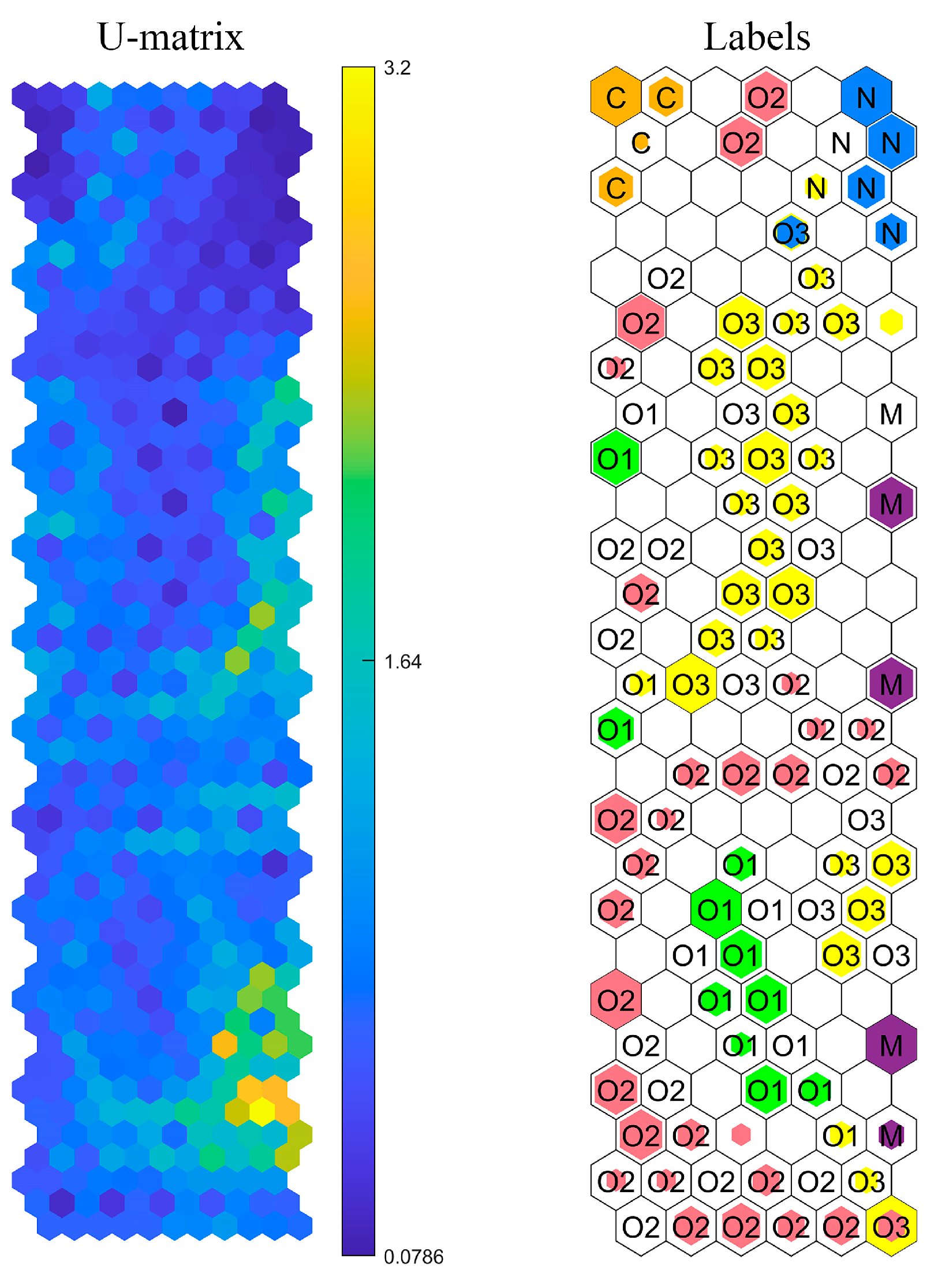
One of the results is illustrated in Figure 10. The U-matrix presents the distance between different neurons. The color shift from blue to yellow denotes an increase in distance value. The letters “N, O, C, and M” in hexagons mean the normal state, bearing outer race fault, cage fault and mixed fault, respectively. The trained SOM neural network can identify which neuron the input testing data should be located in. The colors “blue, green, pink, yellow, orange, and purple” represent testing samples of the normal state, outer race fault in Bearing 1_1, outer race fault in Bearing 1_2, outer race fault in Bearing 1_3, cage fault and mixed fault, respectively. It is obvious that the majority of the samples fell into the right hexagon with the exception of a few samples. It is also possible to determine which fault type the misclassified samples belong to by analyzing the U-matrix and labeled neurons.

The testing results of the trained diagnosis model under five-fold cross-validation is presented in

Table 6. Diagnosis accuracy of the proposed method under five-fold cross-validation.

Fault Type	Test 1 (%)	Test 2 (%)	Test 3 (%)	Test 4 (%)	Test 5 (%)
Normal	97.50	90.00	92.50	95.00	85.00
Outer race fault_1 (Bearing 1_1)	100.00	100.00	93.94	93.94	96.97
Outer race fault_2 (Bearing 1_2)	97.59	96.39	97.59	93.98	98.80
Outer race fault_3 (Bearing 1_3)	84.13	93.65	96.83	95.24	93.65
Cage fault (Bearing 1_4)	100.00	100.00	100.00	96.15	100
Mixed fault (Bearing 1_5)	100.00	100.00	100.00	100	90.91

, and an overall accuracy of 95.99% was achieved. The results showed that the developed method based on the IPVH and SOM could also achieve excellent performance on classification and visualization, in addition to its degradation assessment capability.

4.2. Case 2: Rotary Torsional Fatigue Test

4.2.1. Experiment Setup

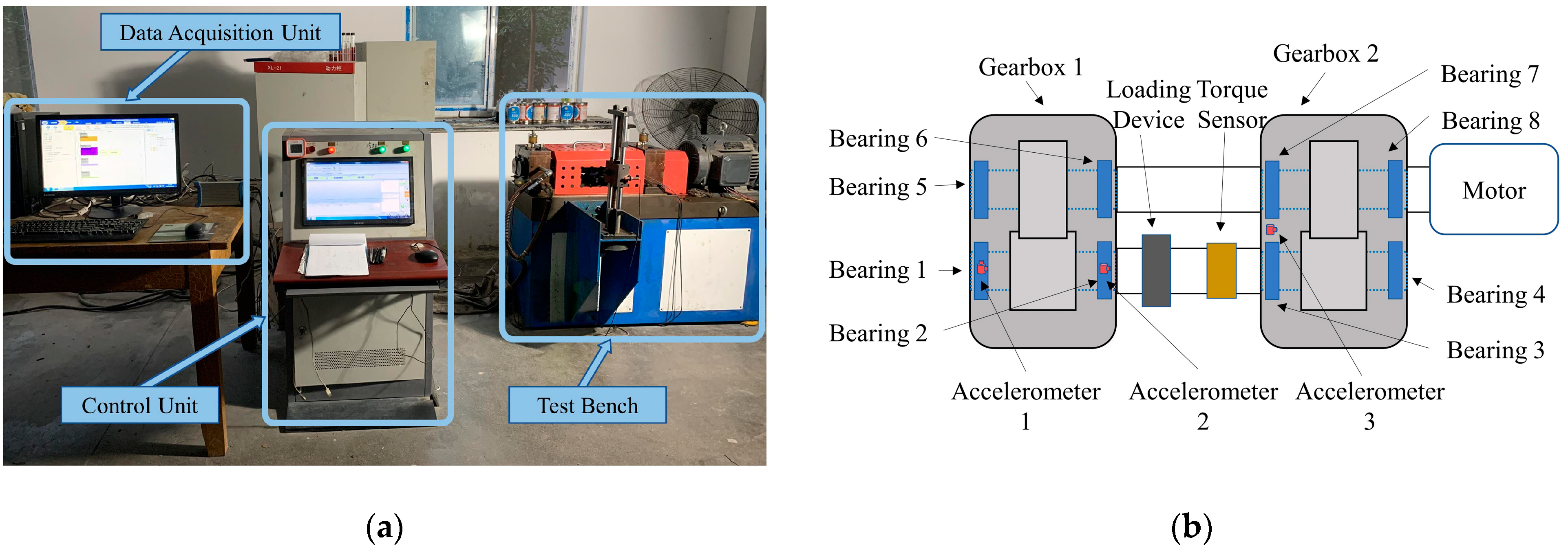
A rotary torsional fatigue test, which is presented in Figure 11a, was devoted to proving the validity of the proposed method in practical engineering application, which is mainly composed of a data acquisition unit, a control unit and a test bench. The data acquisition unit was utilized to collect vibration signals. The required rotating speed and specified torque in the test can be adjusted by the control unit.

The structural composition of the test bench is illustrated in Figure 11b. It mainly consisted of a motor, a torque sensor, a loading device and two gearboxes. An 11 kw three-phase induction motor acted as a drive. The torque needed could be adjusted by the torque sensor and loading device. A pair of gears with 17 and 19 teeth in gearbox 1 was the gears used for the test. Two pairs of bearings were deployed in each gearbox. To acquire the vibration signal, three accelerometers were placed on the gearboxes, where accelerometers 2 and 3 collected vertical signals and accelerometer 1 collected both vertical and horizontal signals. In total, four channels of vibration signals were acquired with the sampling frequency at 20 kHz. Two-second-long vibration signals were collected every 10 min.

As shown in Figure 12, two sets of vibration data were obtained to validate the developed method, which were named Dataset 1 and Dataset 2. A detailed description of the data is listed in

Table 7. Data description of the rotary torsional fatigue test.

Dataset	Working Condition		Fault Type
	Rotating Speed (rpm)	Working Load (Nm)
Dataset 1	1480	400	Mixed bearing fault
Dataset 2	1480	420	Gear pitting

. The vibration signals of Dataset 1 were collected from the vertical direction of accelerometer 1 under the working load of 400 Nm, and the signals of Dataset 2 were collected from the horizontal direction of accelerometer 2 under the working load of 420 Nm. The rotating speed for both was 1480 rpm. When the experiment was finished, as shown in Figure 13, compound faults of the bearing including an inner race fault, outer race fault and ball fault were discovered in the experiment of Dataset 1, and gear pitting was discovered in the experiment of Dataset 2.

4.2.2. Degradation Assessment

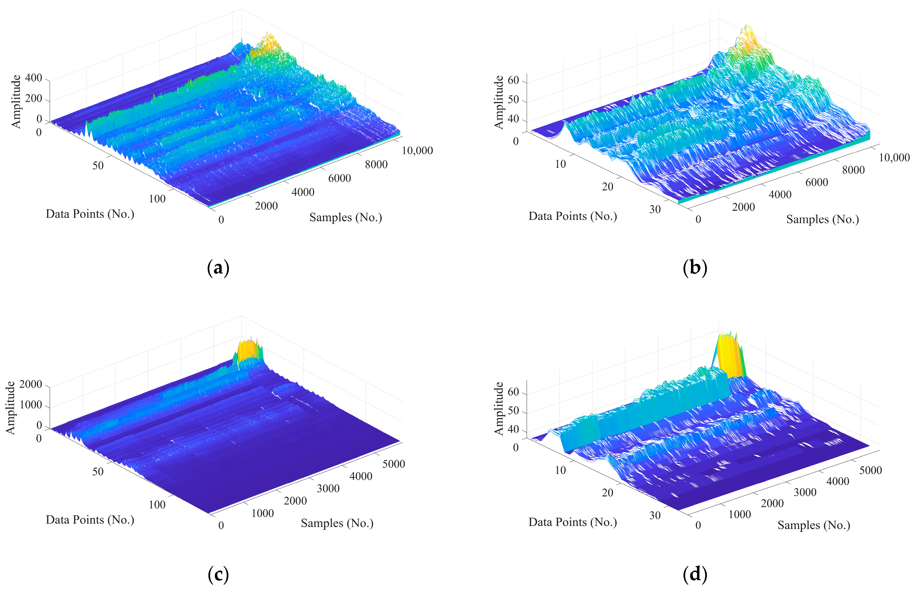
As shown in Figure 14, the same IPVH method used in Section 4.1.2 was implemented to transform the two vibration datasets into 128-dimensional sub-band features and then they were hashed into 32-dimensional MCHs.

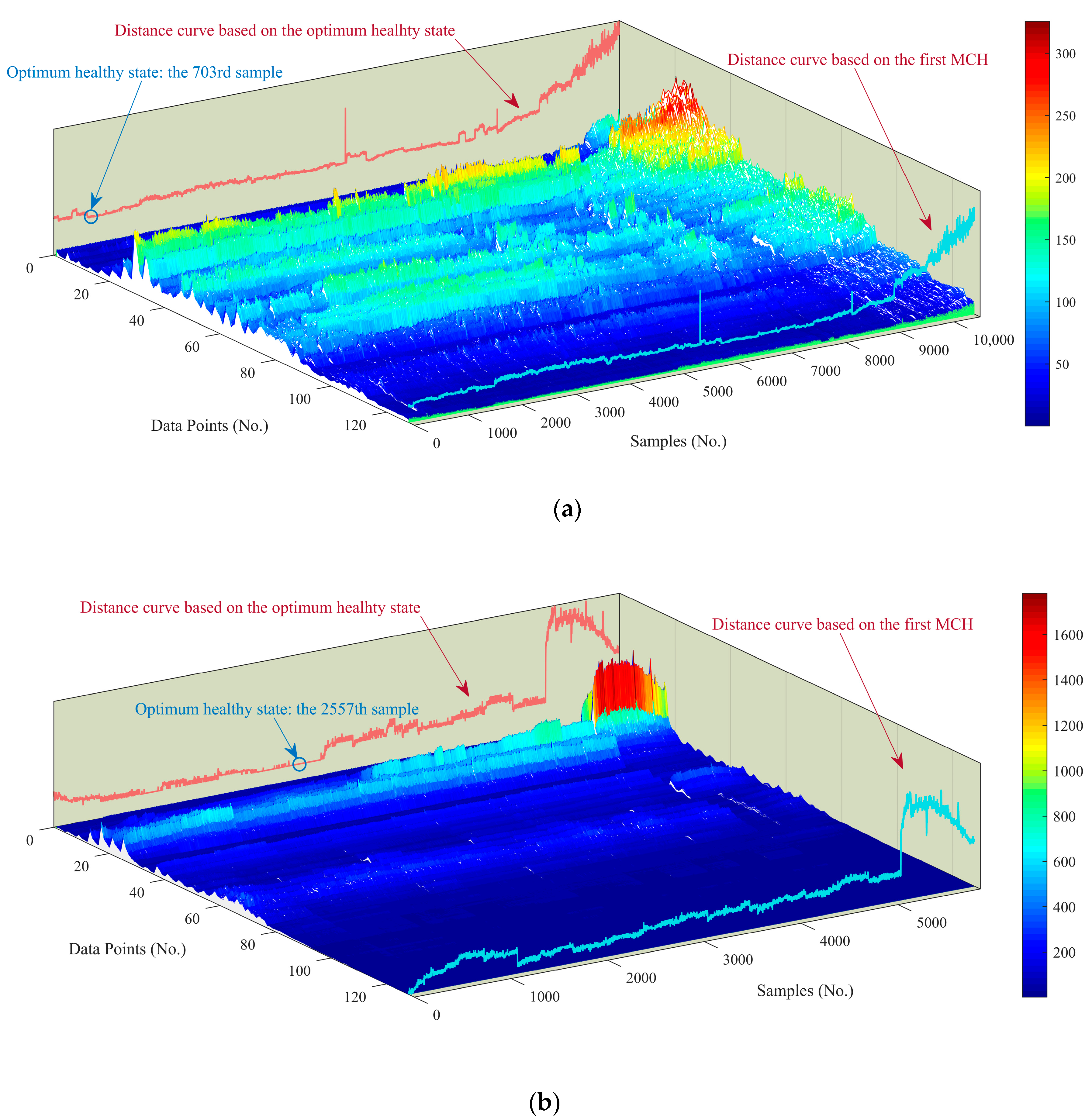
In this part, the, the $\theta$ was set as 200, which means the OHS was updated with every 200 new samples collected. The threshold of changing rates was set as 4%. As is shown in Figure 15 and

Table 8. Results of OHS selection.

Dataset	Total Quantity of Samples	Quantity of Samples Put into the SOM Network	Sample Located in the Clustering Center of SOM Network
Dataset 1	10,473	1000	703rd
Dataset 2	5843	3200	2557th

, when the selection of the OHS was finished, the quantity of the samples put into the SOM and which sample was located in the clustering center are given.

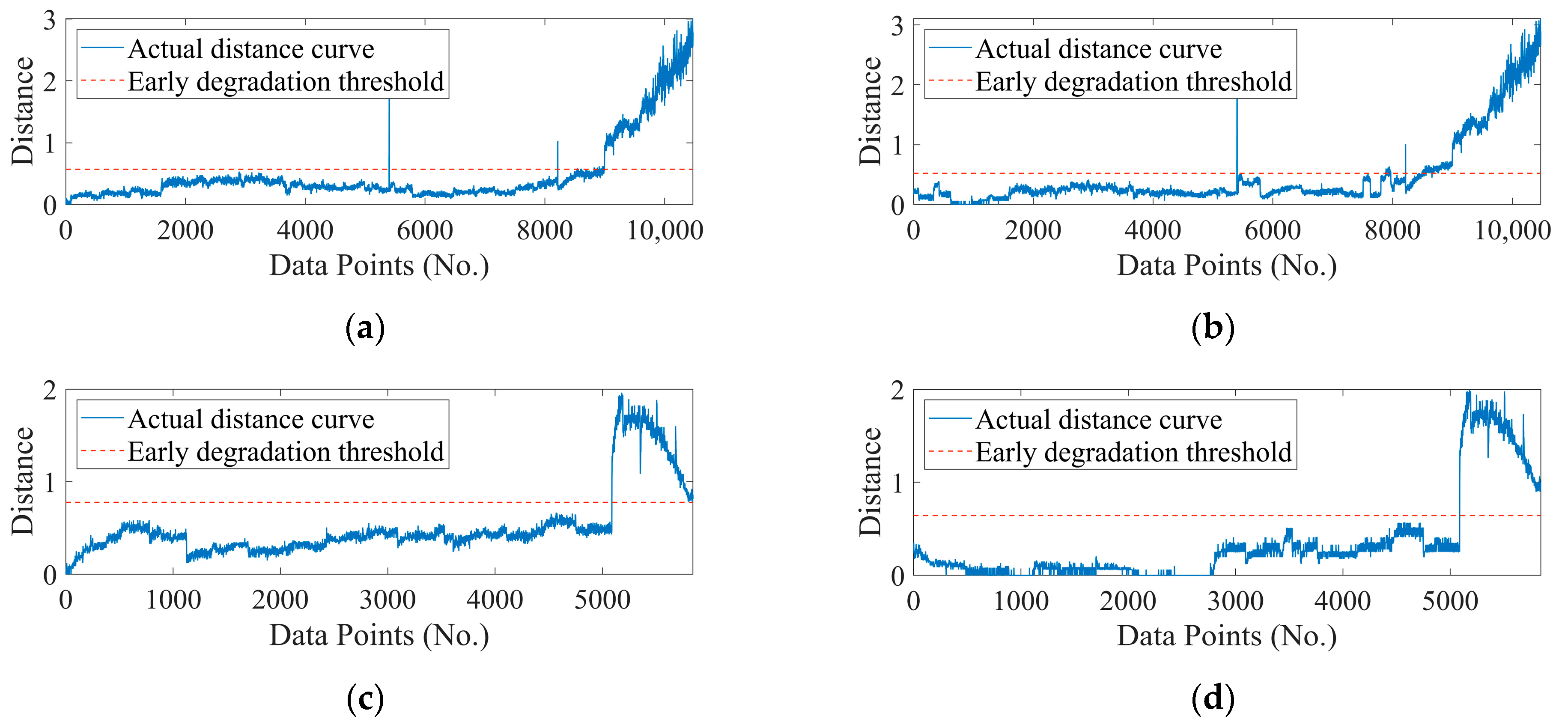
As shown in Figure 16, the distance curves based on different baselines are illustrated. As listed in

Table 9. Quantitative comparison of early degradation detection results.

Dataset	Early Degradation Detection
	Distance Curve Based on the First Sample	Distance Curve Based on the OHS
Dataset 1	8543	7884
Dataset 2	5088	5088

, the distance curve based on the OHS could achieve a comparative earlier degradation detection.

To further illustrate the effectiveness of the proposed scheme for degradation assessment, as shown in Figure 17a, the distance curve based on the OHS was more sensitive to the overall fluctuation in the frequency domain compared with the one based on the first sample. In Figure 17b, for the distance curve based on the OHS, the run-in period is clearly illustrated, whose trend was more consistent with the bathtub curve. For the amplitude increment in the low-frequency band around the 3000^th sample, the distance curve based on the OHS was more sensitive to capturing its changes. However, in the distance curve based on the first sample, when early degradation occurred, some weak fluctuation was always neutralized or averaged out of the existence of the run-in period, which prevents the distance curve from accurately reflecting its true tendency.

4.2.3. Fault Diagnosis

When the distance metric exceeded the preset threshold, in this part, 300 pieces of MCHs were selected from each machine condition, including healthy state, gear pitting and mixed bearing fault. A five-fold cross-validation method was used. For each fault type, as shown in

Table 10. Fault types and sample size for training and testing SOM on rotary torsional fatigue test.

Fault Type	Samples in Total	Training Samples	Testing Samples
Healthy state	300	240	60
Mixed bearing fault	300	240	60
Gear pitting	300	240	60

, four folds including 240 samples were selected to train the SOM network and one fold including 60 samples was left to test the trained diagnostic model.

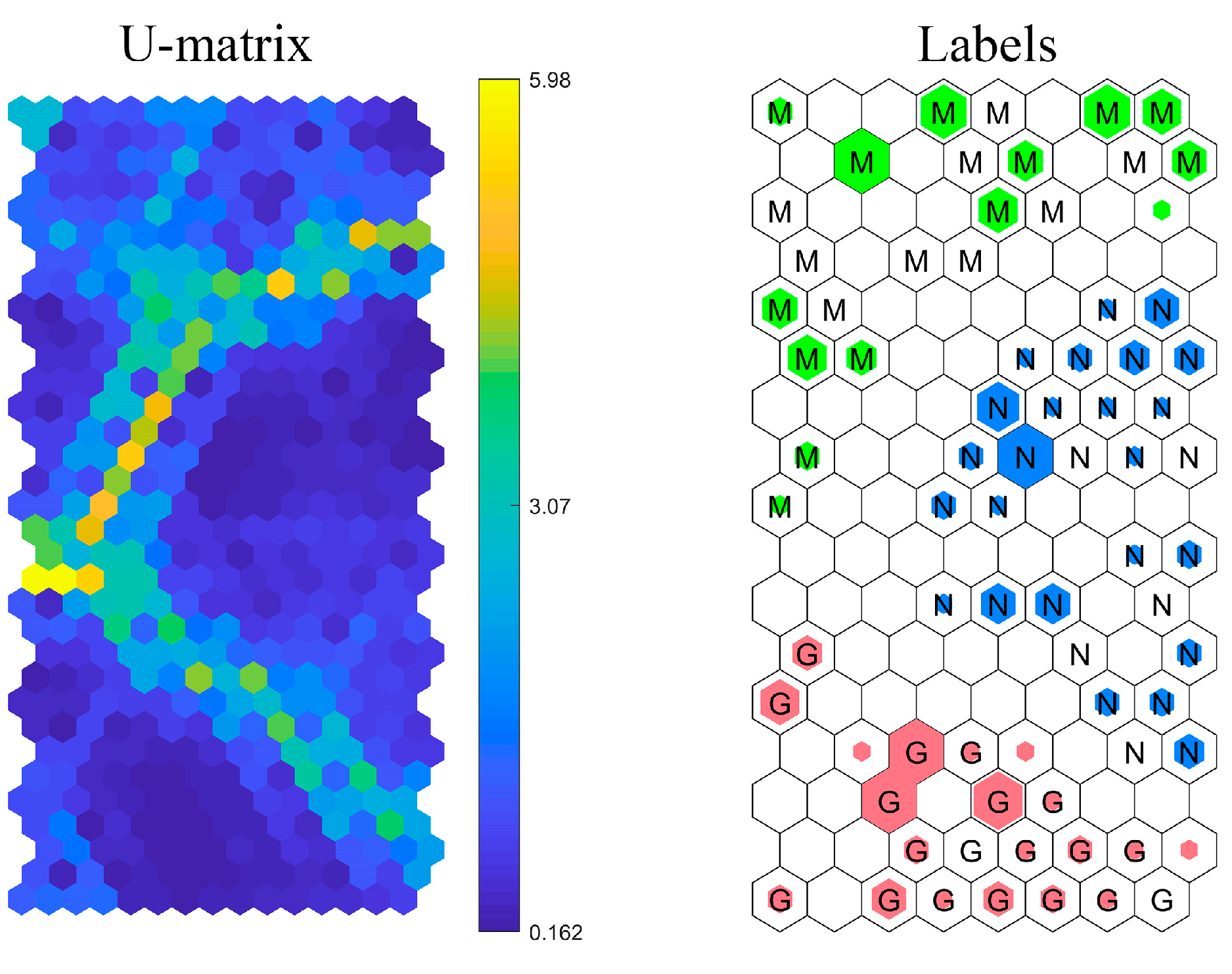
Through the same method in Section 4.1.3, all training data were put into the SOM network, and then the testing data were put into the trained SOM network. As is shown in Figure 18, the colors blue, pink and green represent the normal state (N), mixed bearing fault (M) and gear pitting (G), respectively. Most of the machine conditions were correctly recognized. Diagnosis results under five-fold cross-validation are presented in

Table 11. Diagnosis accuracy of the proposed method on the rotary torsional fatigue test.

Fault type	Test 1 (%)	Test 2 (%)	Test 3 (%)	Test 4 (%)	Test 5 (%)
Normal	100.00	96.67	96.67	93.33	100.00
Mixed fault	98.33	95.00	100.00	98.33	96.67
Gear pitting	95.00	91.67	100.00	100.00	100.00

. The proposed fault diagnosis method could achieve an overall diagnosis accuracy of 97.44%.

5. Conclusions

This paper proposes an integrated condition monitoring method for rotating machinery based on the IPVH and SOM. Firstly, in terms of the issue that the existing methods always focus on either degradation assessment or fault diagnosis, the proposed method achieves both under one technical framework, which improves the efficiency of the whole condition monitoring process. Secondly, for degradation assessment, the run-in period exists because of the influence of temperature, assembly accuracy or other reasons, which indicates that the best machine condition is not always the state at the beginning of the operation. Experimental results showed that the distance metric based on the OHS could achieve a more stable indication of the machine condition and a more robust performance on detecting early degradation compared with features extracted from the time domain and distance metric based on the first sample. Moreover, the degradation trend was always neutralized or averaged in the distance metric based on the first sample, which makes it hard to reflect the degradation process accurately. The distance curve based on the OHS reflected the deviation of the current state from the best machine condition, which could alleviate the issue effectively. Thirdly, for fault diagnosis, when the distance curve exceeded the threshold for identifying early degradation, the corresponding MCHs needed to be transmitted to the diagnostic SOM neural network for machine condition recognition. Through the experiment validation, the proposed fault diagnosis method based on the IPVH and SOM could achieve a 95.99% and 97.44% average classification accuracy and good visualization performance, respectively. It also has implications for further work such as more intelligent methods to select the OHS and the remaining useful life prediction based on the distance metric combined with the OHS.

References

1. Chen, C.; Xue, P.; Fan, X.; Wang, C.; Diao, D. Friction-Induced Rapid Restructuring of Graphene Nanocrystallite Cap Layer at Sliding Surfaces: Short Run-in Period. Carbon 2018, 130, 215–221. [Google Scholar] [CrossRef]
2. Knauder, C.; Allmaier, H.; Salhofer, S.; Sams, T. The Impact of Running-in on the Friction of an Automotive Gasoline Engine and in Particular on Its Piston Assembly and Valve Train. Proc. Inst. Mech. Eng. Part J J. Eng. Tribol. 2018, 232, 749–756. [Google Scholar] [CrossRef] [Green Version]
3. Rausand, M.; Hoyland, A. System Reliability Theory: Models, Statistical Methods, and Applications; John Wiley & Sons: Hoboken, NJ, USA, 2003; ISBN 978-0-471-47133-2. [Google Scholar]
4. Xin, Y.; Li, S.; Cheng, C.; Wang, J. An Intelligent Fault Diagnosis Method of Rotating Machinery Based on Deep Neural Networks and Time-Frequency Analysis. J. Vibroeng. 2018, 20, 2321–2335. [Google Scholar] [CrossRef] [Green Version]
5. Bai, R.; Xu, Q.; Meng, Z.; Cao, L.; Xing, K.; Fan, F. Rolling Bearing Fault Diagnosis Based on Multi-Channel Convolution Neural Network and Multi-Scale Clipping Fusion Data Augmentation. Measurement 2021, 184, 109885. [Google Scholar] [CrossRef]
6. Elasha, F.; Ruiz-Cárcel, C.; Mba, D.; Kiat, G.; Nze, I.; Yebra, G. Pitting Detection in Worm Gearboxes with Vibration Analysis. Eng. Fail. Anal. 2014, 42, 366–376. [Google Scholar] [CrossRef]
7. Liu, G.; Bao, H.; Han, B. A Stacked Autoencoder-Based Deep Neural Network for Achieving Gearbox Fault Diagnosis. Math. Probl. Eng. 2018, 2018, e5105709. [Google Scholar] [CrossRef] [Green Version]
8. Wang, L.; Zhao, X.; Wu, J.; Xie, Y.; Zhang, Y. Motor Fault Diagnosis Based on Short-Time Fourier Transform and Convolutional Neural Network. Chin. J. Mech. Eng. 2017, 30, 1357–1368. [Google Scholar] [CrossRef]
9. Wang, Z.; Zhao, W.; Du, W.; Li, N.; Wang, J. Data-Driven Fault Diagnosis Method Based on the Conversion of Erosion Operation Signals into Images and Convolutional Neural Network. Process Saf. Environ. Prot. 2021, 149, 591–601. [Google Scholar] [CrossRef]
10. Tao, H.; Wang, P.; Chen, Y.; Stojanovic, V.; Yang, H. An Unsupervised Fault Diagnosis Method for Rolling Bearing Using STFT and Generative Neural Networks. J. Frankl. Inst. 2020, 357, 7286–7307. [Google Scholar] [CrossRef]
11. Manhertz, G.; Bereczky, A. STFT Spectrogram Based Hybrid Evaluation Method for Rotating Machine Transient Vibration Analysis. Mech. Syst. Signal Process. 2021, 154, 107583. [Google Scholar] [CrossRef]
12. Liang, P.; Deng, C.; Wu, J.; Yang, Z.; Zhu, J.; Zhang, Z. Compound Fault Diagnosis of Gearboxes via Multi-Label Convolutional Neural Network and Wavelet Transform. Comput. Ind. 2019, 113, 103132. [Google Scholar] [CrossRef]
13. Almounajjed, A.; Sahoo, A.K.; Kumar, M.K. Diagnosis of Stator Fault Severity in Induction Motor Based on Discrete Wavelet Analysis. Measurement 2021, 182, 109780. [Google Scholar] [CrossRef]
14. Sun, Y.; Li, S.; Wang, X. Bearing Fault Diagnosis Based on EMD and Improved Chebyshev Distance in SDP Image. Measurement 2021, 176, 109100. [Google Scholar] [CrossRef]
15. Boškoski, P.; Gašperin, M.; Petelin, D.; Juričić, Đ. Bearing Fault Prognostics Using Rényi Entropy Based Features and Gaussian Process Models. Mech. Syst. Signal Process. 2015, 52–53, 327–337. [Google Scholar] [CrossRef]
16. Udmale, S.S.; Patil, S.S.; Phalle, V.M.; Singh, S.K. A Bearing Vibration Data Analysis Based on Spectral Kurtosis and ConvNet. Soft Comput. 2019, 23, 9341–9359. [Google Scholar] [CrossRef]
17. Liu, H.; Wang, Y.; Li, F.; Wang, X.; Liu, C.; Pecht, M.G. Perceptual Vibration Hashing by Sub-Band Coding: An Edge Computing Method for Condition Monitoring. IEEE Access 2019, 7, 129644–129658. [Google Scholar] [CrossRef]
18. Widodo, A.; Yang, B.-S. Application of Relevance Vector Machine and Survival Probability to Machine Degradation Assessment. Expert Syst. Appl. 2011, 38, 2592–2599. [Google Scholar] [CrossRef]
19. Lei, Y.; Li, N.; Gontarz, S.; Lin, J.; Radkowski, S.; Dybala, J. A Model-Based Method for Remaining Useful Life Prediction of Machinery. IEEE Trans. Reliab. 2016, 65, 1314–1326. [Google Scholar] [CrossRef]
20. Dong, S.; Wu, W.; He, K.; Mou, X. Rolling Bearing Performance Degradation Assessment Based on Improved Convolutional Neural Network with Anti-Interference. Measurement 2020, 151, 107219. [Google Scholar] [CrossRef]
21. Xue, Y.; Dou, D.; Yang, J. Multi-Fault Diagnosis of Rotating Machinery Based on Deep Convolution Neural Network and Support Vector Machine. Measurement 2020, 156, 107571. [Google Scholar] [CrossRef]
22. Dhiman, H.S.; Deb, D.; Muyeen, S.M.; Kamwa, I. Wind Turbine Gearbox Anomaly Detection Based on Adaptive Threshold and Twin Support Vector Machines. IEEE Trans. Energy Convers. 2021, 36, 3462–3469. [Google Scholar] [CrossRef]
23. Kohonen, T. The Self-Organizing Map. Proc. IEEE 1990, 78, 1464–1480. [Google Scholar] [CrossRef]
24. Hu, J.; Zhang, L.; Liang, W. Dynamic Degradation Observer for Bearing Fault by MTS–SOM System. Mech. Syst. Signal Process. 2013, 36, 385–400. [Google Scholar] [CrossRef]
25. Saucedo-Dorantes, J.J.; Delgado-Prieto, M.; Romero-Troncoso, R.D.J.; Osornio-Rios, R.A. Multiple-Fault Detection and Identification Scheme Based on Hierarchical Self-Organizing Maps Applied to an Electric Machine. Appl. Soft Comput. 2019, 81, 105497. [Google Scholar] [CrossRef]
26. Keogh, E.; Chakrabarti, K.; Pazzani, M.; Mehrotra, S. Dimensionality Reduction for Fast Similarity Search in Large Time Series Databases. Knowl. Inf. Syst. 2001, 3, 263–286. [Google Scholar] [CrossRef]
27. Apostolico, A.; Bock, M.E.; Lonardi, S. Monotony of Surprise and Large-Scale Quest for Unusual Words. J. Comput. Biol. 2003, 10, 283–311. [Google Scholar] [CrossRef] [Green Version]
28. Chegini, S.N.; Manjili, M.J.H.; Bagheri, A. New Fault Diagnosis Approaches for Detecting the Bearing Slight Degradation. Meccanica 2020, 55, 261–286. [Google Scholar] [CrossRef]
29. Wang, B.; Lei, Y.; Li, N.; Li, N. A Hybrid Prognostics Approach for Estimating Remaining Useful Life of Rolling Element Bearings. IEEE Trans. Reliab. 2020, 69, 401–412. [Google Scholar] [CrossRef]
Figure 2. Flowchart of the proposed condition monitoring framework.
Machines 10 01025 g002
Figure 3. An overview of the test bench.
Machines 10 01025 g003
Figure 4. Raw vibration signals used in this paper. (a) Bearing 1_1, (b) Bearing 1_2, (c) Bearing 1_3, (d) Bearing 1_4, (e) Bearing 1_5.
Machines 10 01025 g004
Figure 5. Waterfall plots of sub-band features and corresponding MCHs for signals. (a) Sub-band features of Bearing 1_1, (b) MCHs of Bearing 1_1, (c) sub-band features of Bearing 1_2, (d) MCHs of Bearing 1_2, (e) sub-band features of Bearing 1_3, (f) MCHs of Bearing 1_3, (g) sub-band features of Bearing 1_4, (h) MCHs of Bearing 1_4, (i) sub-band features of Bearing 1_5, (j) MCHs of Bearing 1_5.
Machines 10 01025 g005aMachines 10 01025 g005b
Figure 6. Changing rates of RMS. (a) Bearing 1_1, (b) Bearing 1_2, (c) Bearing 1_3, (d) Bearing 1_4, (e) Bearing 1_5.
Machines 10 01025 g006
Figure 7. Distance curves based on the first sample: (a) Bearing 1_1, (c) Bearing 1_2, (e) Bearing 1_3, (g) Bearing 1_4, (i) Bearing 1_5; distance curves based on the OHS sample: (b) Bearing 1_1, (d) Bearing 1_2, (f) Bearing 1_3, (h) Bearing 1_4, (j) Bearing 1_5.
Machines 10 01025 g007
Figure 8. The standard deviation of distance curves in the healthy stage based on various baselines.
Machines 10 01025 g008
Figure 9. Results of early degradation detection using other healthy indexes: (a) Bearing 1_1, (b) Bearing 1_2, (c) Bearing 1_3, (d) Bearing 1_4, (e) Bearing 1_5. Four commonly used features are utilized to be compared with the proposed method. Methods of RMS and peak-to-peak value can achieve similar effectiveness on degradation trend, but it is not sensitive enough to weak degradation. Methods of crest factor and kurtosis are very easily influenced by fluctuation and are even unable to capture the correct degradation trend.
Machines 10 01025 g009
Figure 10. Illustration of training and testing results of SOM.
Machines 10 01025 g010
Figure 11. Experiment setup: (a) experiment equipment, (b) detailed schematic diagram of the test bench.
Machines 10 01025 g011
Figure 12. Illustration of the raw vibration signal. (a) Dataset 1, (b) Dataset 2.
Machines 10 01025 g012
Figure 13. Fault type in Dataset 1: (a) outer race fault, (b) inner race fault, (c) ball fault; fault type in Dataset 2: (d) gear pitting.
Machines 10 01025 g013
Figure 14. Waterfall plots of sub-band features and corresponding MCHs for signals: (a) sub-band features of Dataset 1, (b) MCHs of Dataset 1, (c) sub-band features of Dataset 2, (d) MCHs of Dataset 2.
Machines 10 01025 g014
Figure 15. Changing rates of RMS: (a) Dataset 1, (b) Dataset 2.
Machines 10 01025 g015
Figure 16. Distance curves calculated based on the first MCH: (a) Dataset 1, (c) Dataset 2; distance curves calculated based on the OHS: (b) Dataset 1, (d) Dataset 2.
Machines 10 01025 g016
Figure 17. Comparison among feature maps and distance curves based on different baselines: (a) Dataset 1, (b) Dataset 2.
Machines 10 01025 g017
Figure 18. Illustration of training and testing results of SOM.
Machines 10 01025 g018