Prediction of Aero-Engine Remaining Useful Life Combined with Fault Information

Abstract

Since the fault information of an aero-engine is very important for the remaining useful life of an aero-engine, the paper proposes to combine the fault information for the remaining useful life prediction of an aero-engine. Firstly, we preprocessed the signals of the dataset. Next, the preprocessed signals were used to train a CNN (convolutional neural network)-based fault diagnosis model and obtain fault features from the model. Then, we combined BIGRU (bidirectional gated recurrent unit) and the fault features to predict the remaining useful life of the aero-engine. We used the CMAPSS (commercial modular aviation propulsion system simulation) dataset to verify the effectiveness of the proposed method. After that, comparison experiments with different parameters, structures, and models were conducted in the paper.

1. Introduction

Aero-engine accidents will lead to casualties and irreversible serious consequences. To prevent accidents, we must make timely and effective predictions of the remaining useful life of aero-engines.

RUL (remaining useful life) prediction methods are generally divided into the model-based method, data-driven method, and hybrid method (the combination of the former two methods). For example, Jiao [1] first used two LSTM (long short-term memory network) to extract two features from monitoring data and maintenance data, respectively, and then stacked the two features and sent them to the full connection layer to obtain the health index, and then built the state space model of the health index and obtained the RUL through extrapolation. The PSW (phase space warping) describes the dynamic behavior of the bearing tested on the fast time scale. As a physical-based model, the Paris crack propagation model describes the defect propagation of the bearing on the slow time scale. Qian [2] completed the RUL prediction of the bearing by combining the enhanced PSW with the modified Paris crack propagation model and comprehensively used the information of the fast time scale and the slow time scale. Because the complex working conditions and internal mechanisms hinder the construction of physical models, it is difficult to implement model-based experimental RUL prediction. Since the data-driven method only needs to use historical monitoring data, the data-driven method is receiving more and more attention. In recent years, due to the rapid development of big data and computing power, artificial intelligence has been paid more and more attention and is widely used in RUL prediction.

A variety of artificial intelligence methods have been applied to predict the remaining useful life. Manjurul Islam [3] defined a degree of defect (DD) metric in the frequency domain and inferred the health index of the bearing. Then, according to the health index and the least squares support vector machine, the start times (TTS) point of RUL prediction was obtained, and then the RUL of the bearing was obtained by using the cyclic least squares support vector regression (recurrent LSSVR). Yu [4] used the multi-scale residual temporal convolutional networks (MSR-TCN) to extract the information of multiple scales to more comprehensively analyze health status, and combined this with the attention mechanism to avoid the impact of low correlation data in the prediction process to carry out the engine RUL prediction. Zhang [5] selected 14 sensor signals as the original signals, and through the multi-objective evolutionary ensemble learning method, evolved the multiple DBN (deep belief network) at the same time and took accuracy and diversity as two conflicting goals. After that, the final diagnosis model was obtained by combining multiple DBNs and achieved better results than several different models.

Because the number used in RUL prediction is mostly time-series data and RUL is also time-series related, RNN (recurrent neural networks) with stronger processing ability for time-series data are widely used in RUL prediction. Zheng [6] obtained the health factors by feature selection and PCA, and then combined the health factors and label input LSTM to predict the remaining useful life. Wu [7] selected the sensor data by using monotonicity and correlation, and then completed the prediction of the remaining useful life of the aero-engine by combining the LSTM optimized by the grid search algorithm. Peng [8] used VAE-GAN (variational autoencoder-generative adversarial networks) to generate the health index of the current state, and then used BLSTM (bidirectional long short-term memory) to generate the future sequence sensor data, and then obtained the health index according to the current state and the future state and extrapolated it to obtain RUL.

A variety of methods are adopted to improve the accuracy and speed of remaining life prediction. For example, the accuracy and speed of remaining useful life prediction are improved through some network structure changes [9,10,11]. However, it is not easy to change the network structure according to the appropriate problems to improve the performance. It is easier to improve the prediction accuracy by enriching the state information. Therefore, many methods use a simpler way of enriching state information to improve prediction accuracy. Various approaches are used to enrich the state information and thus improve the prediction accuracy, such as extracting multiple features [12,13,14,15,16], extracting multi-channel features [17,18,19,20], extracting both spatial and temporal features, extracting multi-scale features [21,22,23], and considering the temporal and spatial dependence of sensors [24].

Since different faults will lead to different degradation patterns, the fault features as important state information are very import for the remaining useful life prediction accuracy. Considering that different faults will lead to different degradation modes, Xia [25] established a model based on the state data under each fault state and then used the outputs of the models of multiple degradation modes to obtain the final result. Cheng [26] used two outputs of a transferable convolutional neural network (TCNN) to obtain the fault mode and RUL, respectively. Chen [27] proposed that the degradation pattern of bearings should be classified into slow degradation and fast degradation according to RMS. Then, the BLSTM and attention mechanism were used for remaining useful life prediction. At present, the prediction of the remaining useful life of the engine combined with the fault information has not been paid enough attention. Moreover, the above method does not directly extract the fault features and enrich the fault features as independent information, which will lead to the different degradation mode information being not obvious, and thus reducing the diagnosis accuracy of different degradation modes.

In order to involve the fault features as independent information in the remaining useful life prediction, the paper first uses CNN as a fault diagnosis network to classify faults and obtain fault features from them. Then, a remaining useful life prediction model based on BIGRU and the attention mechanism is developed and combined with the fault features for remaining useful life prediction.

2. Theory

2.1. CNN

CNN is widely used in fault diagnosis due to its outstanding feature extraction ability and the possibility of transforming low-level features into high-level features through a multi-level structure. A typical CNN generally includes an input layer, a convolutional layer, a pooling layer, and a fully connected layer.

The input layer is used to receive raw data. The normalized raw data can improve the efficiency of the algorithm operation.

The convolution layer is used to convolve the output of the previous layer and to activate the convolved data using a nonlinear activation function to learn more advanced features. Its mathematical formula is shown in Formula (1):

$$f_k^{l+1}=f\left({\displaystyle \sum _C{\displaystyle \sum _J{x}_c{}^l(j)\ast w_{k,c}^l+b_k{}^l}}\right)$$

(1)

where $f_i^{l+1}$ is the output corresponding to the k-th convolution kernel of the L-th convolution layer, C represents the number of channels’ input by the convolution layer, $x_c{}^l(j)$ represents the input of the c-th channel of the L-th convolution layer, J represents the j-th local area input for this purpose, $w_{k,c}^l$ represents the weight of the c-th channel of the k-th convolution kernel of the L-th convolution layer, $\ast$ represents convolution, and $b_k^l$ represents the bias of the k-th convolution kernel of the L-th convolution layer. F represents a nonlinear activation function, such as ReLU and sigmoid.

After nonlinear mapping of data by a nonlinear activation function, the data are downsampled by a pooling operation to reduce network parameters. The average pooling takes the average in the perceptual domain as the output. The average pooling formula is shown in Formula (2):

$$P_k^{l+1}=mean\left\{p_k^l\left(t\right)\right\}$$

(2)

where $P_k^{l+1}$ represents the output of the k-th channel of the l-th layer, and $p_k^l\left(t\right)$ represents the t-th region of the output of the k-th channel of the l-th layer.

After passing through multiple convolution layers and pooling layers, the learned features are flattened into vectors, and then the full connection layer is used to connect the extracted features with the output layer. The calculation formula of the full connection layer is shown in Formula (3):

$$y_{}^{l+1}=f\left(x^l\ast w_{}^l+b^l\right)$$

(3)

where $y_{}^{l+1}, x^l$ are, respectively, the input and output of the full connection layer of layer L, f is the activation function, such as softmax, ReLU, etc., and $w_{}^l,b^l$ are, respectively, the weight and bias of the full connection layer of layer L.

2.2. BIGRU

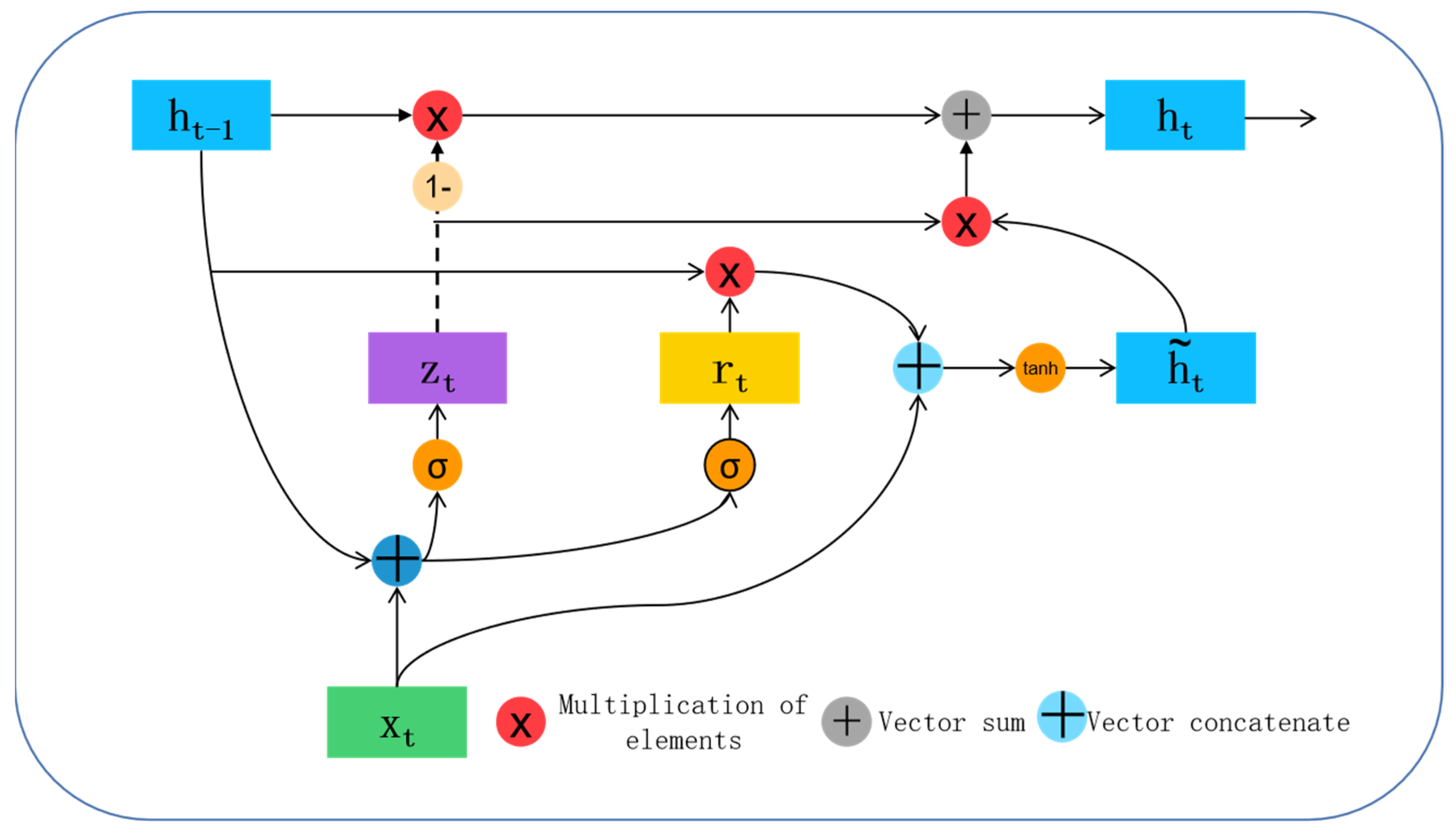
In this paper, we used BIGRU to extract bidirectional temporal information of features. BIGRU has been widely used in natural language recognition and fault diagnosis [28,29]. BIGRU is composed of two independent GRU layers. The input of GRU layers is the same, but the direction of information transmission is the opposite. Compared with the standard GRU, BIGRU can comprehensively consider the historical and future information, thus enhancing the prediction ability. GRU is a variant of RNN. By introducing a gating mechanism to adjust the path of information flow, GRU can effectively solve the problem of gradient explosion in RNN. Moreover, compared with LSTM (another variant of RNN), which can also effectively solve gradient explosion, GRU has higher accuracy and efficiency in predicting the remaining useful life of aero-engines [30]. The structure of the GRU unit is shown in Figure 1.

Figure 1 shows the internal deployment structure of GRU. $h_{t-1}$ represents the hidden state at the previous time, that is, historical information, ${\tilde{h}}_t$ represents the candidate hidden state at the current time, $h_t$ represents the hidden state at the current time, $x_t\in R^f$ (f represents the number of features) represents the input at the current time, ${\mathrm{r}}_t$ represents the reset gate, and $z_t$ represents the update gate. Both $r_t$ and $z_t$ value ranges are $\left[0,1\right]$. The value of $r_t$ indicates the degree to which historical information is introduced into the candidate hidden state ${\tilde{h}}_t$ in the calculation process at the current time. If the value of $r_t$ is close to 0, it indicates that historical information is completely ignored. $z_t$ is used to control the proportion of historical information used in the calculation process at the current time. The larger the value of $z_t$, the more historical information is used in the information at the current time. The specific calculation formula is shown in (4):

$$r_t=\sigma \left(W_r\left[x_t,h_{t-1}\right]+b_r\right)$$

(4)

where $x_t$ is the input at time t, $W_r$ is the weight of $r_t$, $b_r$ is the bias of the reset gate, $\left[x_t,h_{t-1}\right]$ is the concat of two vectors, and $\sigma \left(•\right)$ is the $sigmoid$ function. The update gate Z is used to control the proportion of historical information used during the calculation. Similar to the reset gate $r_t$, the larger the value of the update gate $z_t$, the larger the amount of historical information of the loop block used. The calculation formula is as follows (5):

$$z_t=\sigma \left(W_z\left[x_t,h_{t-1}\right]+b_z\right)$$

(5)

where $W_z$ is the weight of $z_t$ and $b_z$ is the bias of the update gate.

The calculation formula of the hidden candidate state h is as follows (6):

$${\tilde{h}}_t=\tanh \left(W_{\tilde{h}}\left[x_t,\left(r_t^{}\cdot h_{t-1}\right)\right]+b_{\tilde{h}}\right)$$

(6)

where $W_{\tilde{h}}$ is the weight of ${\tilde{h}}_t$ and $b_{\tilde{h}}$ is the bias that hides the candidate state. $•$ represents the multiplication of elements.

The calculation formula of the hidden state at the current time is as follows (7):

$$h_t=\left(1-z_t\right)\cdot h_{t-1}+z_t\cdot \tilde{h}$$

(7)

In BIGRU, the same input data are fed to the forward GRU and the backward GRU. It simultaneously calculates ${\overrightarrow{h}}_t$ (forward GRU hidden state) and ${\overleftarrow{h}}_t$ (backward GRU hidden state) at each time step, and then connects the two hidden states for the next calculation. The BIGRU structure is shown in Figure 2.

2.3. Attention

The attention mechanism is a method to quickly select important information from a large amount of information by imitating human attention. Since the prediction of the remaining useful life of an aero-engine requires more information, we need the attention mechanism to select important information from a large amount of information. When the input sequence of LSTM/GRU model is long, it is difficult to obtain the final reasonable vector representation. It assigns different attention weights to the feature vectors to distinguish the importance of features and improve the accuracy of prediction. The attention mechanism calculation formula is shown in Formulas (8)–(11):

$$S=h_t•\left(H{W}_1\right)$$

(8)

$$\alpha =soft\max (S)$$

(9)

$$\mathrm{context}\_vector=H•\alpha$$

(10)

$$Attention\_vector=\left(concat\left(context\_vector,h_t\right)W_2\right)$$

(11)

where $H=\left(h_1,h_2,h_3\cdots h_t\right)\in R^{t\times f}$, t represents the time-series length of the network input, f represents the number of input features, s is the attention score, $\alpha$ is the attention weight, $\mathrm{context}\_vector$ is the hidden state after the attention weight is given, $Attention\_vector$ is the final output of the attention mechanism, and $W_1, W_2$ is the weight of the two fully connected layers.

3. Proposed Methodology

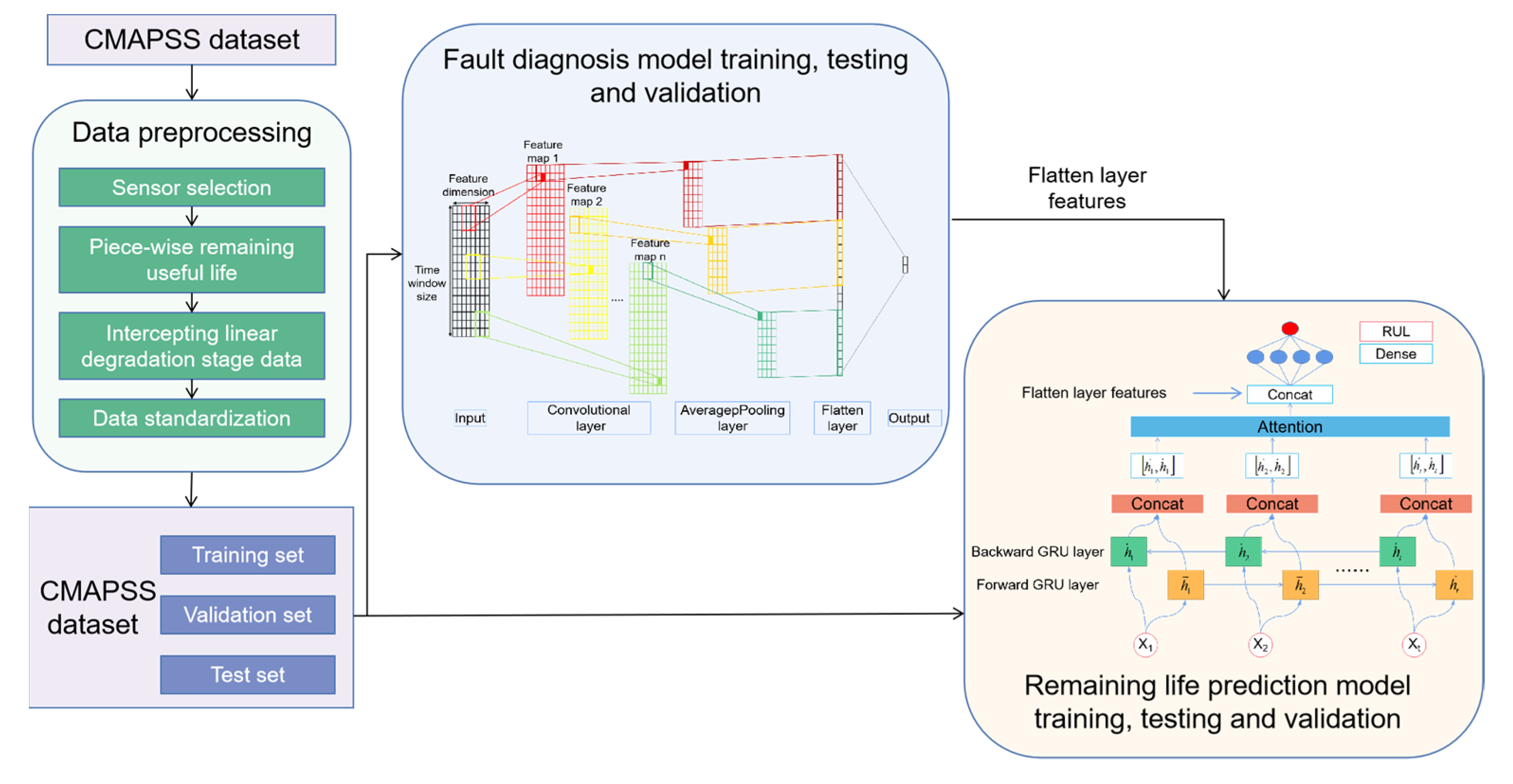
Since different fault states correspond to different degradation patterns, information on fault states is particularly important for remaining useful life predictions. Since previous studies did not directly involve the fault features as independent information in the remaining useful life prediction, the paper proposes to first construct a fault diagnosis model using CNN and obtain the fault features from it. Then, the remaining useful life prediction model based on BIGRU and attention is developed and combined with the fault features to predict the remaining useful life of the engine. The remaining useful life prediction steps combined with fault information are as follows:

• Data preprocessing: We selected 14 sensors related to the degradation trend from 21 sensor signals. Then, the selected 14 sensor signals were normalized so that the influence of the data on the results is on the same scale. After that, the standardized data were further processed by the sliding window method to obtain the sample signal. According to the previous experience, the window length and the step size were, respectively, selected as 30 and 1. According to the expert’s suggestion, the remaining useful life was converted into the segmented remaining useful life, and the maximum remaining useful life is 125. It was assumed in the paper that when the engine is in the linear degradation stage, the data used for fault diagnosis and remaining useful life prediction are in the linear degradation stage. The two types of faults of FD001 and FD003 in the linear degradation stage were assigned different fault labels and combined with the corresponding data to obtain the original fault diagnosis model data. The corresponding sensor data in the linear degradation stage were combined with the remaining useful life labels to obtain the remaining useful life prediction model data.
• Build a fault diagnosis model based on CNN: We stacked 14 sensor signals with a trending effect as the input of a two-dimensional convolutional network. We constructed a layer of convolutional network for feature extraction and a fully connected layer for classification. We chose the cross-entropy loss function and Adam as the loss function and optimizer of the fault diagnosis model, respectively. The output of the flatten layer of the fault diagnosis model was used as fault features for the next step of remaining useful life prediction.
• Build a remaining useful life prediction model combining fault information: We also stacked 14 sensor signals with a trending effect as the model input for remaining life prediction. The BIGRU output layer was selected with an attention mechanism to obtain better features. The output of the attention mechanism and the fault features extracted from the fault diagnosis model were then concatenated as the features of the final remaining useful life prediction model and fed into a two-layer fully connected layer to obtain the remaining useful life. We chose the mean square error (MSE) and Adam as the loss function and optimizer of the remaining useful life prediction model, respectively.

The flow chart of the proposed method for predicting the remaining useful life of an aero-engine combined with fault information is shown in Figure 3.

3.1. Dataset

The dataset used in this paper was the NASA CMAPSS (commercial modular aviation propulsion system simulation) dataset [31]. CMAPSS has been widely used in RUL prediction research of turbofan engines. There are four subsets (FD001, FD002, FD003, and FD004), and each subset records the degradation data of the turbofan engine under different fault modes. We verified the validity of the proposed method using subsets FD001 and FD003. The training set for both FD001 and FD003 contained run-to-failure monitoring data streams for 100 engines of the same type. Their test sets contain the same type of data of the same number of engines. There were one and two faults in the operation of datasets FD001 and FD003, respectively. The length of the condition monitoring data were inconsistent between one engine and another, and it was polluted by the sensor noise, making it a challenging task to predict RUL (in the unit of the operating cycle). The dataset description and the detailed description of the sensor are shown in

Table 1. Dataset description.

Datasets	FD001	FD002	FD003	FD004
Number of training set engines	100	260	100	248
Number of test set engines	100	259	100	248
Operating conditions	1	6	1	6
Faults	1	1	2	2

and

Table 2. Dataset sensor detailed description.

Index	Symbol	Description	Units
1	T2	Total temperature at fan inlet	°R
2	T24	Total temperature at LPC outlet	°R
3	T30	Total temperature at HPC outlet	°R
4	T50	Total temperature at LPT outlet	°R
5	P2	Pressure at fan inlet	psia
6	P15	Total pressure in bypass-duct	psia
7	P30	Total pressure at HPC outlet	psia
8	Nf	Physical fan speed	rpm
9	Nc	Physical core speed	rpm
10	epr	Engine pressure ratio (P50/P2)	--
11	Ps30	Static pressure at HPC outlet	psia
12	phi	Ratio of fuel flow to Ps30	pps/psi
13	NRf	Corrected fan speed	rpm
14	NRc	Corrected core speed	rpm
15	BPR	Bypass ratio	--
16	farB	Burner fuel–air ratio	--
17	htBleed	Bleed enthalpy	--
18	Nf_dmd	Demanded fan speed	rpm
19	PCNfR_dmd	Demanded corrected fan speed	rpm
20	W31	HPT coolant bleed	lbm/s
21	W32	LPT coolant bleed	lbm/s

.

3.2. Sensor Selection

Each engine corresponds to a series of data points sampled by 21 sensors over its life cycle. Of the 21 sensors, some have a constant output over the life of the engine and do not provide any useful information for remaining life prediction. Therefore, as conducted in [5,32], we eliminated the outputs of these sensors from the C-MAPSS dataset. Therefore, we finally selected 14 features in the C-MAPSS dataset, corresponding to the outputs of 14 sensors, with indexes of 2, 3, 4, 7, 8, 9, 11, 12, 13, 14, 15, 17, 20, and 21.

3.3. Piecewise Remaining Useful Life

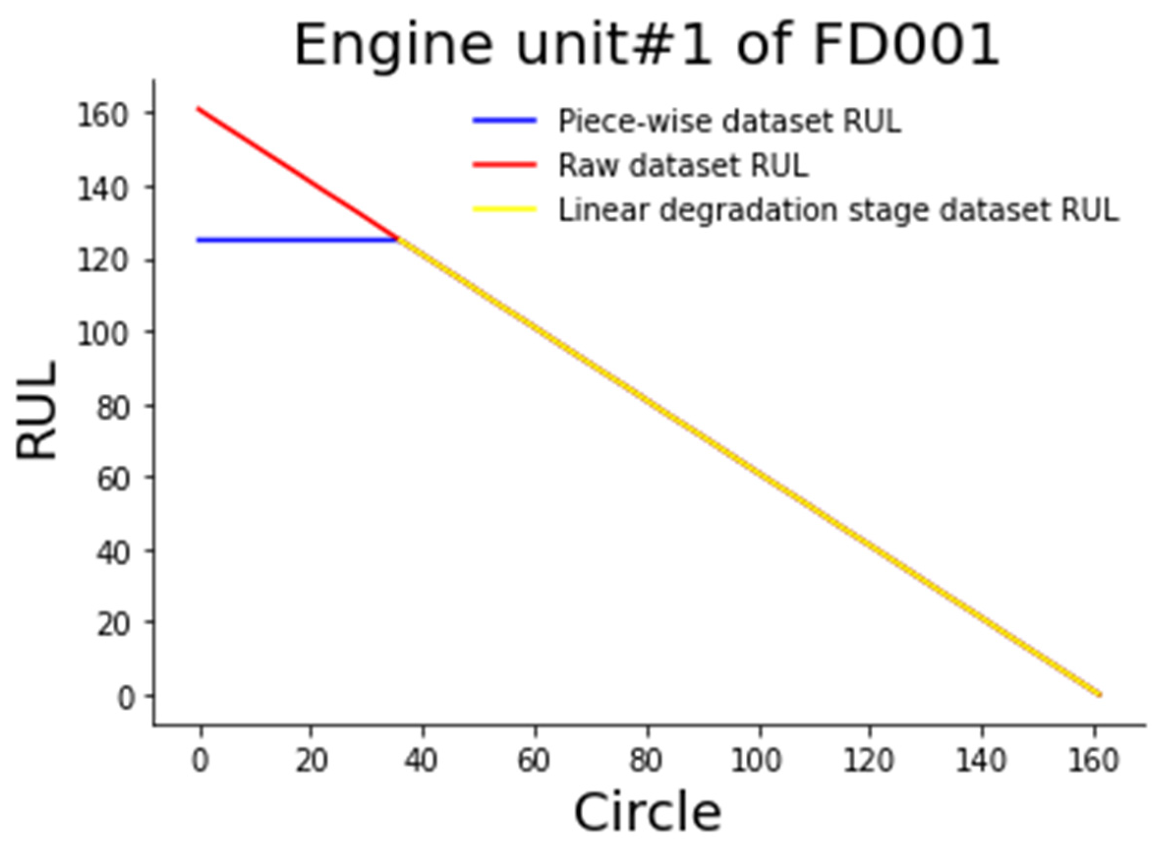
Since the engine works stably and linearly in the early stage, it stops working until the system fails. Here, we used the usual label processing method, i.e., the piecewise linear label, which assigns a constant value to the target label of the early monitoring signal (for the C-MAPSS dataset, 125 was used as the constant RUL label) [33,34,35]. Zheng [36] limited the RUL of the engine from start-up to degradation to within RULmax. The linear degradation of an aero-engine occurs after RULmax. In this work, RULmax was set to 125.

3.4. Intercepting Linear Degradation Stage Data

Since a fault occurs in the dataset when the operation reaches a certain point in time, only the data from the linear degradation phase where we believe the engine has experienced the fault described in the dataset were taken in the paper. The two fault modes of FD001 and FD003 were assigned two different fault labels to form the fault diagnosis data. The remaining useful life prediction data were then formed using the corresponding remaining useful life labels. Taking the first engine of FD001 as an example, the linear degradation stage dataset RUL is shown in Figure 4.

3.5. Data Standardization

Standardization of data before input into the model can greatly improve the accuracy and efficiency of the model. In order to facilitate the application of data in the model, standardization was carried out according to the formula to remove the influence of different dimensions in the linear degradation stage data. The standardization formula is shown in (12):

$$x_{norm}^{i,j}=\frac{\left(x^{i,j}-{\mu }^j\right)}{{\sigma }^j}$$

(12)

where $x^{i,j}$ is the i-th point of the j-th sensor signal, $x_{norm}^{i,j}$ is the normalized data of the i-th point of the j-th sensor signal, ${\mu }^j$ is the mean value of the j-th sensor signal, and ${\sigma }^j$ is the variance of the j-th sensor signal.

The dataset obtained after processing the collection of FD001 and FD003 training sets by the above steps was divided into training and validation sets in the ratio of 8:2. Meanwhile, the dataset obtained after processing the collection of FD001 and FD003 test sets according to the above steps was used as the test set of the proposed method.

3.6. Evaluation Indicators

RMSE (root mean square error) is used to measure the deviation of the predicted value from the true value. The smaller the RMSE value, the closer the true value is to the predicted value. Since it is often used to evaluate the CMPASS dataset, RMSE was used as the final evaluation metric in the paper. The formula of RMSE is shown in (13):

$$RMSE=\sqrt{\frac{1}{n}{\displaystyle \sum _{i=1}^n{\left(RU{L}_{i,predicted}-RU{L}_{i,true}\right)}^2}}$$

(13)

where n represents the predicted total number, $RU{L}_{i,predicted}, RU{L}_{i,true}$ represent the predicted remaining useful life and the real remaining useful life, respectively.

4. Experimental Results and Analysis

4.1. Fault Diagnosis Model Results

In order to extract fault information for remaining useful life prediction, the paper constructed a CNN-based fault diagnosis network to extract fault features. The output features of the fault diagnosis model flatten layer were used as fault information for the next step of remaining useful life prediction.

The parameters of the fault diagnosis model are shown in

Table 3. The parameters of the fault diagnosis model.

Layer	Input	Output	Filters	Kernel Size	Strides	Padding	Activation
Input	(30, 14, 1)	(30, 14, 1)
2D-Conv	(30, 14, 1)	(16, 30, 14, 1)	16	(3, 3)	1	Same	ReLU
Average pooling	(16, 30, 14, 1)	(16, 15, 7, 1)		(2, 2)	2	Same
Flatten	(16, 15, 7, 1)	(1680)
Dense	(1680)	(2)					softmax

.

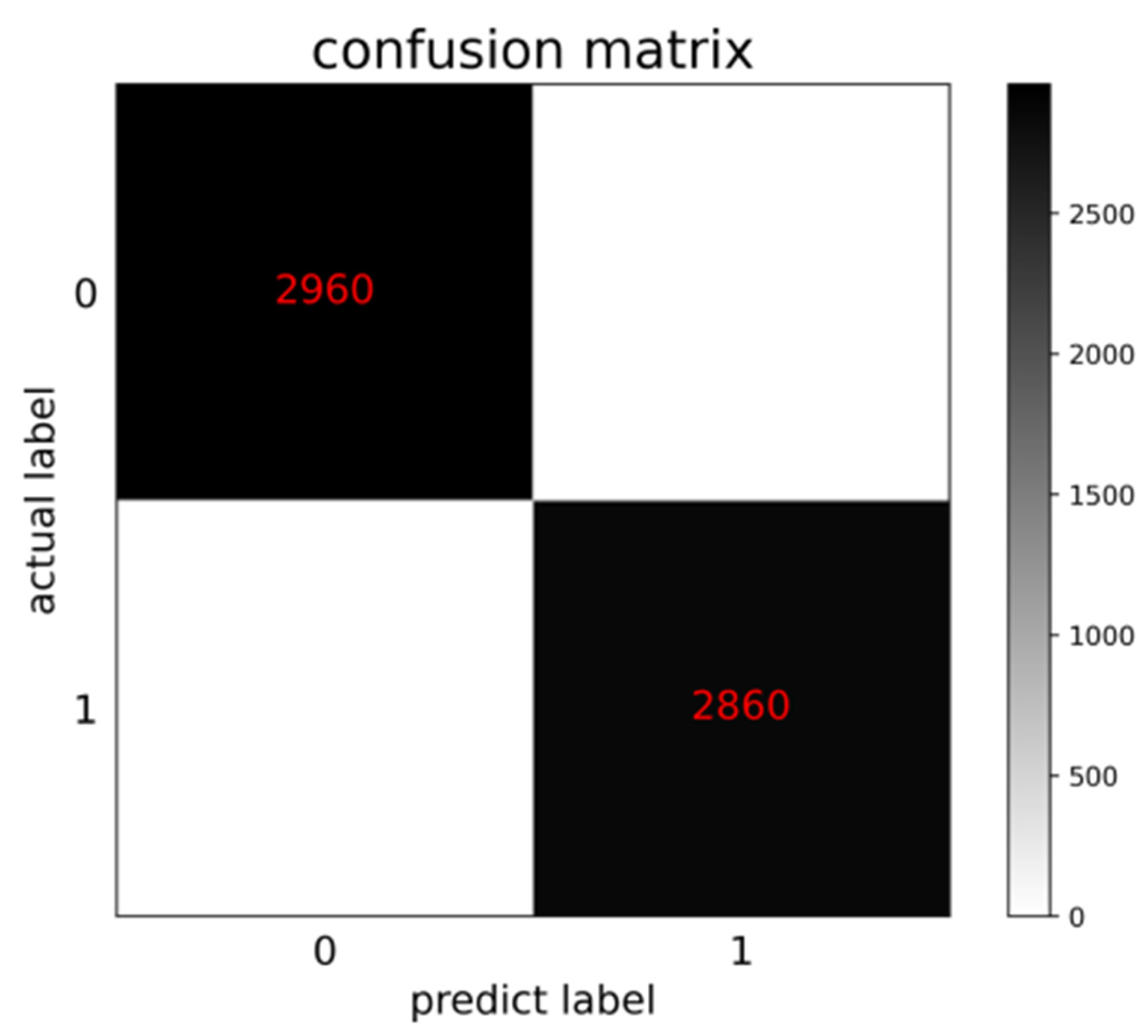
We validated the performance of the model using the test sets. The confusion matrix of the test results of the fault diagnosis model on the test set is shown in Figure 5. The horizontal axis represents the prediction label of the test sets. The vertical axis represents the real label of the test sets. Additionally, the main diagonal represents the correct number of samples predicted by the model. It can be seen that the test accuracy of the model reaches 100%. The generalization ability of the model is verified. The performance of the model is verified.

4.2. Comparative Test and Analysis of Influencing Factors of Fault Diagnosis Model

4.2.1. Comparative Experimental Analysis of the Number of Convolution Kernels

To verify the reasonableness of the number of convolutional kernels, comparison experiments were conducted on four numbers of convolutional kernels, 2, 4, 8, and 16.

The results in

Table 4. Comparative experimental analysis of the number of convolution kernels.

Number of Convolution Kernels	Test Accuracy
2	99.58%
4	99.98%
8	99.99%
16	100%

show that the highest testing accuracy of the model was achieved when the number of convolutional kernels is 16. It is also clear from the data in the table that as the number of convolutional kernels increases, both the variety of features extracted and the testing accuracy improve. The comparison of the experimental results shows that the number of convolutional kernels chosen in the paper is reasonable.

4.2.2. Comparative Experimental Analysis of Convolution Layers

To verify the reasonableness of the number of convolutional layers, comparison experiments were conducted on three convolutional layers, 1, 2, and 3.

From the results in

Table 5. Comparative experimental analysis of convolution layers.

Number of Convolution Layers	Test Accuracy
1	100%
2	97.21%
3	99.94%

, it can be seen that the test accuracy of the fault diagnosis model reaches the highest when the number of convolutional layers is 1. The reasonableness of the number of convolutional layers selected in the paper is verified.

4.2.3. Comparative Experimental Analysis of Convolution Activation Function

To verify the rationality of the activation function of the convolutional layer, a comparison experiment between two activation functions, ‘tanh’ and ‘ReLU’, was conducted.

From the results in

Table 6. Comparative experimental analysis of convolution activation function.

Activation Function	Test Accuracy
tanh	99.94%
ReLU	100%

, it can be seen that the highest testing accuracy of the model was achieved when the activation function is ‘ReLU’. The reasonableness of the activation function selected in the paper is verified.

4.3. Prediction Results of Remaining Useful Life

Since different fault states lead to different degradation patterns, the paper constructed a CNN-based fault diagnosis model and extracted fault information from it. Then, the remaining useful life prediction model based on BIGRU and the attention mechanism was combined with the fault information for remaining useful life prediction.

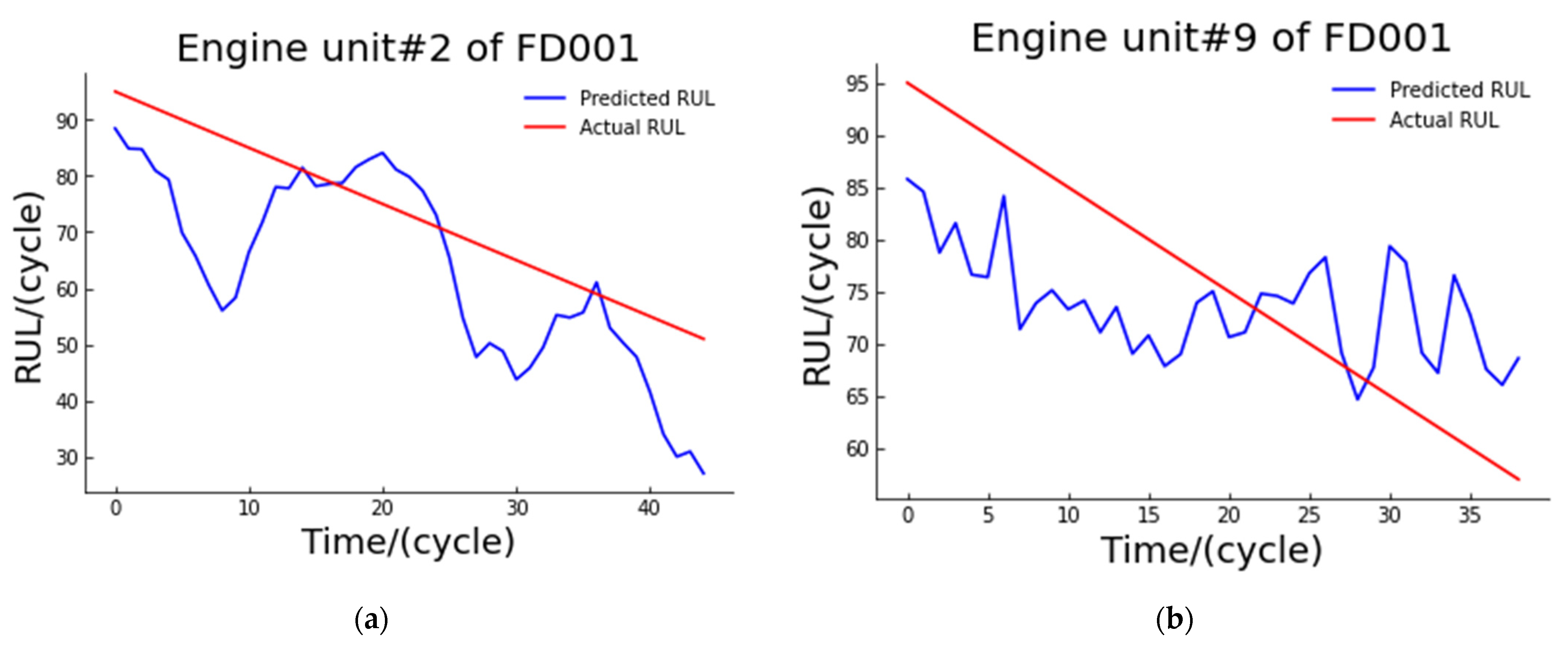
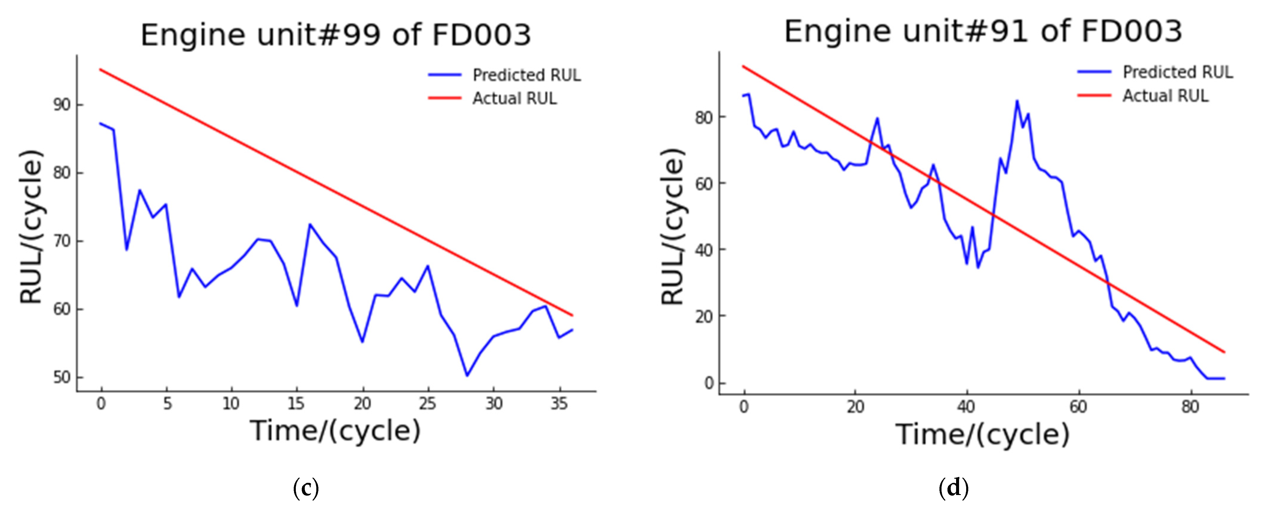
The following figures (Figure 6) show the actual degradation curves and model predicted degradation curves for the two engines selected from the test sets of FD001 and FD003, respectively.

The overall RMSE of the dataset on the model was 11.046, and the minimum MSE of the model reached 0.911.

4.4. Comparison Test and Analysis of Influencing Factors of Prediction Model

The parameters of the remaining useful life prediction model are shown in

Table 7. The parameters of the remaining useful life prediction model.

Layer	Input	Output	Number of Hidden Units	Activation
Input	(30, 14)	(30, 14)
BIGRU	(30, 14)	(30, 64)	32
Attention	(30, 64)	(64)
Concat	(64), (1680)	(1744)
Dense	(1744)	(4)		ReLU
Dense	(4)	(1)		ReLU

.

In this section, we investigated the effect of different factors (GRU uni- and bi-directional, attention mechanism, number of hidden units, and fault information) by comparing different existing methods.

When analyzing certain factors, other factors were set as default values. See the table for default values. The frameworks used in this paper were Python 3.8.8 and tensorflow 2.3.

4.4.1. Necessity Analysis of Bidirectional Network and Attention Mechanism

In this section, in order to verify the necessity of bidirectional networks and attention mechanisms for improving the accuracy of remaining lifetime prediction, we conducted comparative experiments of A-GRU, A-BIGRU, and BIGRU to analyze the necessity of bidirectional networks and attention mechanisms (

Table 8. Comparison results of bidirectional network and attention mechanisms.

Network	RMSE	The Percent Improvement
BIGRU	11.485	3.82%
A-GRU	12.164	9.19%
A-BIGRU	11.046

).

From the comparison of RMSE results of A-GRU and A-BIGRU, it can be seen that when the model is a bidirectional network, the RMSE of the model is lower, which means that the predicted value is closer to the real value. It can be concluded that when the network is bidirectional, the remaining useful life prediction model can combine the information from both time directions to make a more accurate prediction of the remaining useful life of the engine. The comparison of the RMSE results from A-BIGRU and BIGRU also shows that the remaining lifetime prediction accuracy is higher when the attention mechanism is added to the model. The percent improvement in the table is the percentage improvement of the method mentioned in the paper compared to the corresponding method. By comparing the experimental results, it can be concluded that the bidirectional network and the attention mechanism are necessary to improve the accuracy of the model.

4.4.2. Comparison of the Number of Hidden Cells of A-BIGRU Network

To verify the rationality of the number of hidden units of the A-BIGRU network selected in this paper, we conducted a comparative experiment on the number of four hidden units: 16, 32, 64, and 128.

It can be seen from

Table 9. Comparison of the number of hidden cells of A-BIGRU network.

Number of Hidden Units	RMSE
16	12.362
32	11.046
64	11.477
128	11.388

that when the number of hidden units of the model is 32, the accuracy of the model reaches the highest. When the number of hidden units is too small, it cannot provide rich information for model analysis. When the number of hidden units is too large, the redundancy of information is not conducive to network prediction. Through experimental analysis, it was found that the accuracy of the model reaches the best when the number of hidden units of the model is 32.

4.4.3. Comparison Experiment of Fault Information Presence and Absence

In order to verify the necessity of fault information to improve the accuracy of remaining useful life prediction, this paper conducted a comparison experiment based on eight different network structures with or without adding fault information as the independent variable.

The RMSE results of the remaining useful life prediction model are shown in

Table 10. Comparison experiment of fault information presence and absence.

Networks	RMSE		The Percent Improvement
	Add Fault Information	No Fault Information
GRU	11.585	11.822	2%
BIGRU	11.485	11.558	0.63%
LSTM	11.681	12.377	5.62%
BLSTM	11.442	11.561	1.03%
A-GRU	12.164	12.363	1.61%
A-LSTM	11.689	11.894	1.72%
A-BIGRU	11.046	12.299	10.19%
A-BLSTM	11.659	11.912	2.12%

. It can be seen that the accuracy of the eight network structures increased after the fault information was added, and the most intuitive expression is the decrease in RMS value. The model used in the paper has the largest reduction in RMSE value of 1.254 after combining the fault information, which indicates that the predicted remaining useful life is closer to the actual remaining useful life. The percent improvement in the table is the percentage improvement of the method with fault information relative to the method without fault information. Therefore, it can be concluded that the fault information is important for the remaining useful life prediction. The validity of the method in the paper is verified.

4.4.4. Comparison of Different Methods

In order to better show the advantages of the proposed method, a comparison with several current RUL prediction methods was performed. Since the dataset used in the paper was the collection of FD001 and FD003, the results of several comparison methods were taken as the average of the experimental results of FD001 and FD003. The comparison results are shown in

Table 11. Comparison of different methods.

Methods	RMSE	The Percent Improvement
MSR-TCN [4]	14.1	21.65%
DCNN [33]	12.625	12.21%
GASEN-TCN [7]	13.855	20.27%
TCN [37]	12.125	8.90%
Bi-LSTM-CNN [17]	12.045	8.29%
The proposed method	11.046

.

From the results in Table 11, it can be concluded that the proposed method in the paper has different degrees of advantages over the existing methods. The maximum and minimum RMSE improvement percentages reached 21.65% and 8.29%, respectively.

5. Conclusions

Predicting the remaining useful life of an aero-engine is particularly important to prevent and mitigate risks and improve the safety of life and property. Maximizing the accuracy of the prediction can also provide more reasonable opinions for engine health management and thus take more reasonable maintenance measures.

Different faults correspond to different degradation patterns. However, in the past, the remaining useful life prediction of aero-engines did not sufficiently consider the fault information and involve it as independent information in the remaining useful life prediction. To solve this problem, the paper first classified the engine fault data by CNN to obtain the fault features. Then, the remaining useful life prediction was performed by combining the fault features and the remaining useful life prediction model based on BIGRU and the attention mechanism. After that, comparative experiments of different network structures, parameters, and methods were carried out. The experimental results show that the accuracy of the model is higher, and the parameters used are reasonable. Therefore, it proves that fault information is necessary to predict the remaining useful life of aero-engines.

The data used in the paper were experimental data under the same working conditions. We did not analyze the migration learning for different operating conditions. So, we will work in the direction of remaining useful life prediction with the involvement of fault information of different operating conditions in the future.

References

1. Jiao, R.; Peng, K.; Dong, J. Remaining Useful Life Prediction for a Roller in a Hot Strip Mill Based on Deep Recurrent Neural Networks. IEEE/CAA J. Autom. Sin. 2021, 8, 1345–1354. [Google Scholar] [CrossRef]
2. Qian, Y.; Yan, R.; Gao, R.X. A multi-time scale approach to remaining useful life prediction in rolling bearing. Mech. Syst. Signal Process. 2017, 83, 549–567. [Google Scholar] [CrossRef] [Green Version]
3. Manjurul Islam, M.M.; Prosvirin, A.E.; Kim, J. Data-driven prognostic scheme for rolling-element bearings using a new health index and variants of least-square support vector machines. Mech. Syst. Signal Process. 2021, 160, 107853. [Google Scholar] [CrossRef]
4. Yu, J.; Peng, Y.; Deng, Q. Remaining Useful Life Prediction Based on Multi-Scale Residual Convolutional Network for Aero-Engine; IEEE: Piscataway, NJ, USA, 2021; pp. 1–6. [Google Scholar]
5. Zhang, C.; Lim, P.; Qin, A.K.; Tan, K.C. Multiobjective Deep Belief Networks Ensemble for Remaining Useful Life Estimation in Prognostics. IEEE Trans. Neural Netw. Learn. Syst. 2017, 28, 2306–2318. [Google Scholar] [CrossRef]
6. Zheng, G.; Wu, L.; Wen, T.; Zheng, C.; Wang, C.; Lin, G. Research on Predicting Remaining Useful Life of Equipment Based on Health Index; IEEE: Piscataway, NJ, USA, 2021; pp. 145–149. [Google Scholar]
7. Wu, J.; Hu, K.; Cheng, Y.; Zhu, H.; Shao, X.; Wang, Y. Data-driven remaining useful life prediction via multiple sensor signals and deep long short-term memory neural network. ISA Trans. 2020, 97, 241–250. [Google Scholar] [CrossRef]
8. Peng, Y.; Pan, X.; Wang, S.; Wang, C.; Wang, J.; Wu, J. An Aero-Engine RUL Prediction Method Based on VAE-GAN; IEEE: Piscataway, NJ, USA, 2021; pp. 953–957. [Google Scholar]
9. Qin, Y.; Chen, D.; Xiang, S.; Zhu, C. Gated Dual Attention Unit Neural Networks for Remaining Useful Life Prediction of Rolling Bearings. IEEE Trans. Ind. Inform. 2021, 17, 6438–6447. [Google Scholar] [CrossRef]
10. Fu, S.; Zhong, S.; Lin, L.; Zhao, M. A Novel Time-Series Memory Auto-Encoder With Sequentially Updated Reconstructions for Remaining Useful Life Prediction. IEEE Trans. Neural Netw. Learn. Syst. 2021, 1–12. [Google Scholar] [CrossRef] [PubMed]
11. Cheng, Y.; Hu, K.; Wu, J.; Zhu, H.; Shao, X. Autoencoder Quasi-Recurrent Neural Networks for Remaining Useful Life Prediction of Engineering Systems. IEEE/ASME Trans. Mechatron. 2022, 27, 1081–1092. [Google Scholar] [CrossRef]
12. Li, B.; Tang, B.; Deng, L.; Zhao, M. Self-Attention ConvLSTM and Its Application in RUL Prediction of Rolling Bearings. IEEE Trans. Instrum. Meas. 2021, 70, 1–11. [Google Scholar] [CrossRef]
13. Chen, Z.; Wu, M.; Zhao, R.; Guretno, F.; Yan, R.; Li, X. Machine Remaining Useful Life Prediction via an Attention-Based Deep Learning Approach. IEEE Trans. Ind. Electron. 2021, 68, 2521–2531. [Google Scholar] [CrossRef]
14. Zhang, Z.; Song, W.; Li, Q. Dual-Aspect Self-Attention Based on Transformer for Remaining Useful Life Prediction. IEEE Trans. Instrum. Meas. 2022, 71, 1–11. [Google Scholar] [CrossRef]
15. Xiang, S.; Qin, Y.; Luo, J.; Pu, H.; Tang, B. Multicellular LSTM-based deep learning model for aero-engine remaining useful life prediction. Reliab. Eng. Syst. Saf. 2021, 216, 107927. [Google Scholar] [CrossRef]
16. Liu, Y.; Wang, X. Deep & Attention: A Self-Attention Based Neural Network for Remaining Useful Lifetime Predictions; IEEE: Piscataway, NJ, USA, 2021; pp. 98–105. [Google Scholar]
17. Song, J.W.; Park, Y.I.; Hong, J.; Kim, S.; Kang, S. Attention-Based Bidirectional LSTM-CNN Model for Remaining Useful Life Estimation; IEEE: Piscataway, NJ, USA, 2021; pp. 1–5. [Google Scholar]
18. Amin, U.; Kumar, K.D. Remaining Useful Life Prediction of Aircraft Engines Using Hybrid Model Based on Artificial Intelligence Techniques; IEEE: Piscataway, NJ, USA, 2021; pp. 1–10. [Google Scholar]
19. Zraibi, B.; Okar, C.; Chaoui, H.; Mansouri, M. Remaining Useful Life Assessment for Lithium-Ion Batteries Using CNN-LSTM-DNN Hybrid Method. IEEE Trans. Veh. Technol. 2021, 70, 4252–4261. [Google Scholar] [CrossRef]
20. Liu, H.; Liu, Z.; Jia, W.; Lin, X. Remaining Useful Life Prediction Using a Novel Feature-Attention-Based End-to-End Approach. IEEE Trans. Ind. Inform. 2021, 17, 1197–1207. [Google Scholar] [CrossRef]
21. Miao, M.; Yu, J. A Deep Domain Adaptative Network for Remaining Useful Life Prediction of Machines Under Different Working Conditions and Fault Modes. IEEE Trans. Instrum. Meas. 2021, 70, 1–14. [Google Scholar] [CrossRef]
22. Qin, Y.; Zhou, J.; Chen, D. Unsupervised health Indicator construction by a novel degradation-trend-constrained variational autoencoder and its applications. IEEE/ASME Trans. Mechatron. 2021, 3, 1447–1456. [Google Scholar] [CrossRef]
23. Qin, Y.; Xiang, S.; Chai, Y.; Chen, H. Macroscopic–Microscopic Attention in LSTM Networks Based on Fusion Features for Gear Remaining Life Prediction. IEEE Trans. Ind. Electron. 2020, 67, 10865–10875. [Google Scholar] [CrossRef]
24. Li, T.; Zhao, Z.; Sun, C.; Yan, R.; Chen, X. Hierarchical attention graph convolutional network to fuse multi-sensor signals for remaining useful life prediction. Reliab. Eng. Syst. Saf. 2021, 215, 107878. [Google Scholar] [CrossRef]
25. Xia, P.; Huang, Y.; Li, P.; Liu, C.; Shi, L. Fault Knowledge Transfer Assisted Ensemble Method for Remaining Useful Life Prediction. IEEE Trans. Ind. Inform. 2022, 18, 1758–1769. [Google Scholar] [CrossRef]
26. Cheng, H.; Kong, X.; Chen, G.; Wang, Q.; Wang, R. Transferable convolutional neural network based remaining useful life prediction of bearing under multiple failure behaviors. Measurement 2021, 168, 108286. [Google Scholar] [CrossRef]
27. Chen, Y.; Liu, Z.; Zhang, Y.; Zheng, X.; Xie, J. Degradation-trend-dependent Remaining Useful Life Prediction for Bearing with BiLSTM and Attention Mechanism. In Proceedings of the 2021 IEEE 10th Data Driven Control and Learning Systems Conference (DDCLS), Suzhou, China, 14–16 May 2021; pp. 1177–1182. [Google Scholar]
28. Cheng, Q.; Peng, B.; Li, Q.; Liu, S. A Rolling Bearing Fault Diagnosis Model Based on WCNN-BiGRU; IEEE: Piscataway, NJ, USA, 2021; pp. 3368–3372. [Google Scholar]
29. Di, L.; Xiushuang, Y.; Ling, X. Design of Natural Language Model Based on BiGRU and Attention Mechanism; IEEE: Piscataway, NJ, USA, 2021; pp. 191–195. [Google Scholar]
30. Wang, Y.; Zhao, Y.; Addepalli, S. Practical Options for Adopting Recurrent Neural Network and Its Variants on Remaining Useful Life Prediction. Chin. J. Mech. Eng. 2021, 34, 1–20. [Google Scholar] [CrossRef]
31. Saxena, A.; Goebel, K.; Simon, D.; Eklund, N. Damage Propagation Modeling for Aircraft Engine Run-to-Failure Simulation; IEEE: Piscataway, NJ, USA, 2008; pp. 1–9. [Google Scholar]
32. Lim, P.; Goh, C.K.; Tan, K.C. A Time Window Neural Network Based Framework for Remaining Useful Life Estimation; IEEE: Piscataway, NJ, USA, 2016; pp. 1746–1753. [Google Scholar]
33. Li, X.; Ding, Q.; Sun, J. Remaining useful life estimation in prognostics using deep convolution neural networks. Reliab. Eng. Syst. Saf. 2018, 172, 1–11. [Google Scholar] [CrossRef] [Green Version]
34. Li, Z.; Zheng, Z.; Outbib, R. Adaptive Prognostic of Fuel Cells by Implementing Ensemble Echo State Networks in Time-Varying Model Space. IEEE Trans. Ind. Electron. 2020, 67, 379–389. [Google Scholar] [CrossRef] [Green Version]
35. Hu, K.; Cheng, Y.; Wu, J.; Zhu, H.; Shao, X. Deep Bidirectional Recurrent Neural Networks Ensemble for Remaining Useful Life Prediction of Aircraft Engine. IEEE Trans. Cybern. 2021, 1–13. [Google Scholar] [CrossRef]
36. Zheng, S.; Ristovski, K.; Farahat, A.; Gupta, C. Long Short-Term Memory Network for Remaining Useful Life Estimation; IEEE: Piscataway, NJ, USA, 2017; pp. 88–95. [Google Scholar]
37. Li, R.; Chu, Z.; Jin, W.; Wang, Y.; Hu, X. Temporal Convolutional Network Based Regression Approach for Estimation of Remaining Useful Life; IEEE: Piscataway, NJ, USA, 2021; pp. 1–10. [Google Scholar]
Figure 1. The structure of GRU unit.
Machines 10 00927 g001
Figure 2. The BIGRU structure.
Machines 10 00927 g002
Figure 3. The flow chart of the proposed method experiment.
Machines 10 00927 g003
Figure 4. Linear degradation stage dataset RUL.
Machines 10 00927 g004
Figure 5. The confusion matrix of the test results of the fault diagnosis model.
Machines 10 00927 g005
Figure 6. (a,b) The actual degradation curve and predicted degradation curve of two engines from FD001; (c,d) the actual degradation curve and predicted degradation curve of two engines from FD003.
Machines 10 00927 g006aMachines 10 00927 g006b