Numerical Investigation and Experimental Verification of the Fluid Cooling Process of Typical Stator–Rotor Machinery with a Plate-Type Heat Exchanger

Abstract

This paper discusses the heat transfer process for a typical stator–rotor machinery-hydrodynamic retarder from the perspective of computational fluid dynamics and experimental means. Fluid cooling is an essential step in the working process of hydrodynamic retarders, and changes in viscosity along with temperature rise will affect the performance of braking. To investigate the heat transfer process of stator–rotor machinery, a novel computational fluid dynamics (CFD) method, combined with a dynamic thermophysical property transfer algorithm, is proposed. A heat-flow coupling numerical method with experimental verification is proposed, in which the density and the viscosity are variable with the temperature in an effectiveness–number of transfer units (P-NTU) method. The results show that the numerical results are in good agreement with the experimental data, with a 0.1–2.5% error. The influence of an asymmetric structure on heat transfer characteristics is discussed. The results show that the optimal braking performance, along with the liquid cooling performance, is achieved under outlets with an inlet passage set as 90 degrees.

1. Introduction

With the continual increase in power production of heavy transportation, thermal management has become a challenge for power and transmission systems, thus demanding fluid flow and heat transfer technologies in complex configurations [1]. For a typical auxiliary braking machine, the vehicular hydrodynamic retarders convert kinetic energy into liquid heat, resulting in the generation of braking torque [2]. The thermal–fluid heat transfer efficiency greatly affects the braking performance of the system, and the study of the liquid cooling process is significant for the performance of thermal energy management on heavy vehicles equipped with hydrodynamic retarders.

Generally, to explore internal flow characteristics and predict the external working characteristics of fluid machinery, computational fluid dynamics (CFD) methods with experiment tools are the most often used approaches [3]. The lattice Boltzmann (LB) method [1] is proposed to investigate the influences of exponentially temperature-dependent viscosity on free convection in a porous cavity with a circular cylinder. Mu [4] studied the effect of inlet and outlet flow rates on oil pressures and braking torque by modeling the full flow passage of the working chamber with CFD means. A modified k-ε turbulence model was proposed by Saqr [5] to compute the shear-driven vortex flow in an open cylindrical cavity, and Laser Doppler Anemometry (LDA) measurements with test results demonstrated the validity in computing vortex-dominated flows. The system working characteristics vary with the temperature fluid medium and have been widely investigated. Zhang et al. proposed a novel anisotropic k-ω turbulence model [6] for predicting heat-transfer characteristics in the rotor blade of gas turbines and proved that flow with rotation is more complex than flow without rotating due to the interaction between the Coriolis and the centrifugal buoyancy force. Wang et al. [7] proposed a temperature model based on an artificial neural network to predict the temperature performance of a hydrodynamic retarder. With CFD and test results at different temperatures as inputs, the external performance was predicted and validated in experiments. Liu et al. [8] proposed a computational fluid dynamics method with variable density and viscosity for hydrodynamic retarders, but the effect of the heat exchange process was not taken into consideration. Bu et al. [9] used the user-defined function (UDF) approach to formulate thermophysical properties. It was found that density and viscosity changing with temperature have a great impact on the braking torque. These dynamic thermophysical properties with temperature should be employed in numerical simulations to avoid errors.

To deeply study the mechanism of flow and mass transfer in chambers, variable viscosity assumption has been performed by simulation and experimental means, especially in fluid machinery. To solve the Navier–Stokes equations under the variable viscosity, Martin [10] first used an elegant method for an incompressible fluid of variable viscosity. By introducing the vorticity function and the generalized energy function, the order of the governing equations was reduced from second order to first order. For vorticity distribution, Naeem [11] presented a class of exact solutions of the equations governing the steady plane flows of incompressible fluid of variable viscosity. Fatsis [12] presented an analytical solution to the Navier–Stokes equations in rotating systems with variable viscosity fluids. In addition to these analytical studies, numerical models have been developed by many researchers. Liu et al. [8] compared the experimental and CFD results with constant viscosity and variable viscosity assumptions and demonstrated that, after considering the changes in viscosity with temperature, the predicted braking torque is more precise. Guo et al. [13] analyzed the viscosity effect on the performance of the turbine flowmeter and demonstrated that changes in wake flow behind the upstream-flow conditioner blade are caused by variable viscosity. In ref. [14], a transient simulation method of the variable viscosity–temperature field for a specially shaped cavity was proposed using FLUENT software and was validated with experimental verification results.

As mentioned in ref. [8,14], numerical methods commonly used the user-defined function (UDF) approach to formulate thermophysical properties, which could not reflect the dynamic heat transfer process in a transient simulation. It is of great value to consider the characteristics of the heat exchanger when solving the Navier–Stokes equations in the fluid heat transfer progress. The heat transfer mechanism with the heat exchanger has been investigated in many studies. To study the effects of linearly varying viscosity and thermal conductivity on a steady free convective flow with the essence of a heat exchanger, Mahanti and Gaur [15] transformed governing equations of continuity, momentum, and energy of a viscous incompressible fluid into coupled and non-linear ordinary differential equations with similarity transformation, and then solved it by the Runge–Kutta fourth-order method. The plate type heat exchanger (PHE) is an efficient tool for indirect liquid cooling [16]. An indirect liquid plate heat exchanger (PHX) involves two liquid streams, namely cold fluid and hot fluid in different passages, and the heat transfer process happens when the two streams flow onto an adjacent plate. The plate corrugations are mostly in the form of chevrons. Due to intersections and large flow resistance in this type of corrugation, a notably increased heat transfer effect was observed [17]. The most common analysis models of the heat exchanger include the log mean temperature difference (LMTD) methods [18,19] and the effectiveness–number of transfer units (P-NTU) methods [20]. When the fluid inlet temperatures are known and the outlet temperatures are specified or readily determined from the energy balance expressions, the LMTD method is easy to perform [21]. However, if only the inlet temperatures are known, the application of the LMTD method will lead to a cumbersome iterative procedure. A more appropriate method, namely P-NTU, to solve the heat transfer rating problem was proposed by Kays and London [22]. A dimensionless parameter called the heat exchanger effectiveness, P, is defined to represent the ratio of actual heat transfer rate to the maximum possible heat transfer rate.

Though varying viscosity has been widely studied in the heat transfer process of fluid machinery, few researchers have investigated the effect of asymmetric structures in the heat transfer process. In ref. [23], the authors studied non-uniform inlet flow velocity and obtained asymmetrical velocity profiles in FLEC and attributed asymmetrical results. The heat transfer process over a cylinder symmetrically placed in a sudden expansion channel, which can be regarded as an asymmetric structure, is simulated in ref. [24]. Li et al. [25] investigated the convective mass transfer performance of various asymmetric structures and pointed out that asymmetry flow on flow and mass transfer performance should be focused, which is usually ignored because of people’s inertial assumption about only one symmetric solution for the flow in a symmetrical structure. The various asymmetric structures, along with the various inlet speeds and rotational speeds, easily affect the liquid cooling performance and the working efficiency of the rotation. The effect of asymmetric structures, especially the position of inlet passage and outlet passage and various inlet speeds and rotational speeds, on the heat transfer characteristics should be further investigated. This could direct the optimal design of the thermal management system and instigate the forward design of the flow field of fluid machinery.

To fill the above search gaps, the main contribution of this paper can be summarized as follows:

Firstly, a full flow transient numerical simulation of flow and mass with dynamic heat transfer along with steady analysis for typical stator–rotor fluid machinery is proposed. A bench test is also established to validate the accuracy of the proposed method.

Secondly, the CFD tool combined with the P-NTU method is first used to simulate the oil-filling process of the hydrodynamic retarder. The dynamic heat transfer process is studied by transient simulation with a view towards looking at the temperature field and the viscosity field.

Thirdly, the effect of various asymmetric structures along with inlet flow and rotational speeds on the heat transfer process is investigated. The influence of the structural parameters of the stator–rotor fluid machine on the transient heat transfer phenomenon is first revealed.

2. Materials and Methods

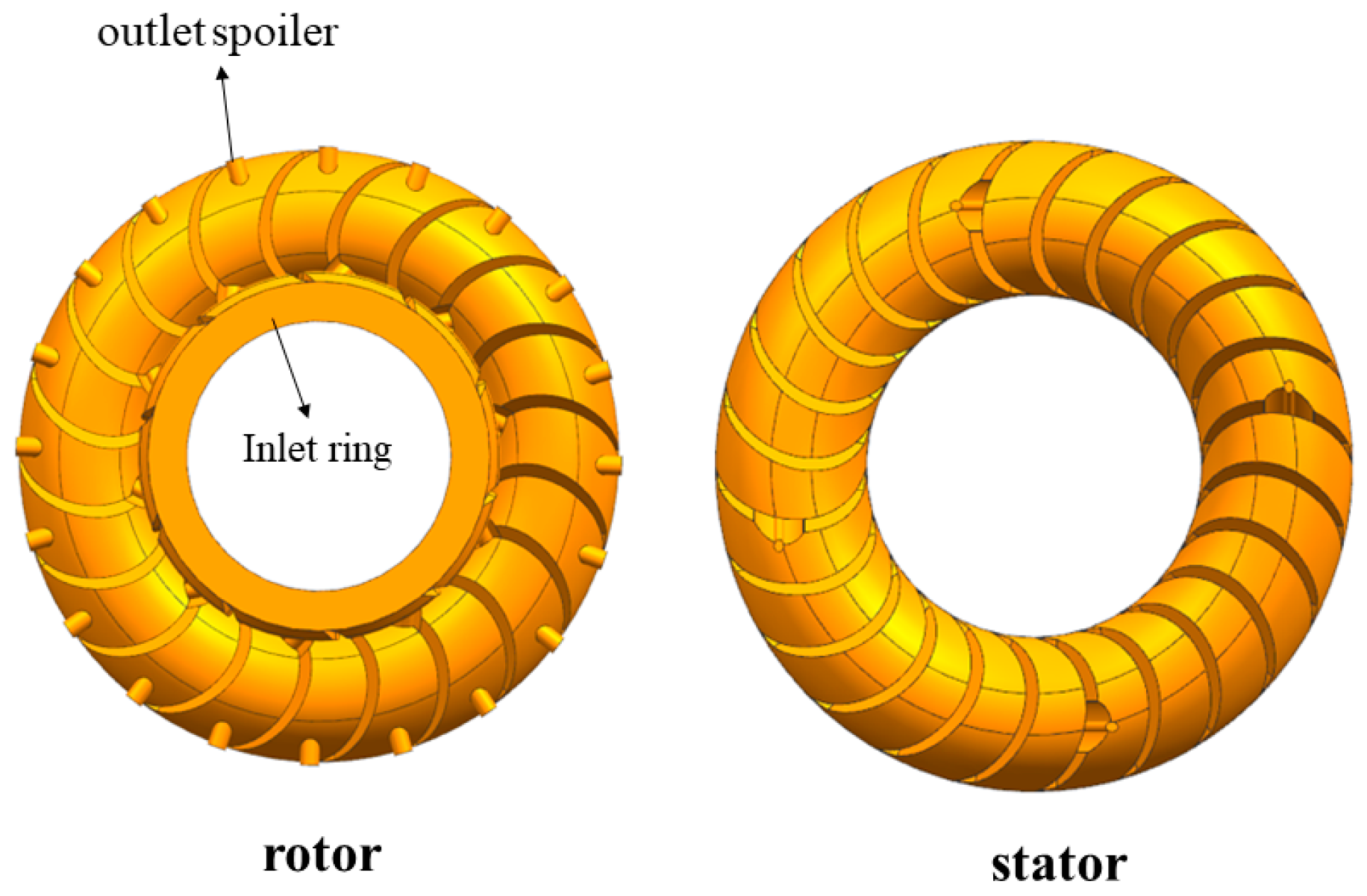
2.1. Structures of Hydrodynamic Retarder

A schematic diagram of the hydrodynamic retarder is depicted in Figure 1; the working chamber is substituted by the hydraulic control system, the cascade part, and the oil-charging and discharging passages. Among the hydraulic control system, the oil-charging valve along with the charging regulation valve linked with the pump, which is controlled by the control oil, decides the filling state of the wheel chamber. Oil outflowing from the outlet will enter the plate-type heat exchanger, then the cold oil flowback will flow into the wheel chamber by the inlet and finish the self-circulation cooling process. The external diameter and internal diameter of the hydrodynamic retarder are 380 mm and 220 mm, respectively. The working chamber structure of the hydrodynamic retarder comprises the rotor, stator, and oil-charging and discharging passages, as well as the hot exchange and oil control systems.

The system oil enters the inlet from the oil-charging valve, which is a switch valve controlled by control oil. For the outlet, the system oil enters and flows back into the bump through the charging regulation valve, which is also named the electric-hydraulic proportional relief valve, to regulate the oil charging rate of the working chamber. System oil is cooled in a self-circulating cooling process, and the plate-type exchanger is used for its high heat transfer coefficient, which meets the liquid cooling requirements of the hydrodynamic retarder.

2.2. Governing Equation

The mass conservation equation is as follows [26]:

$$\frac{\partial \rho }{\partial t}+\frac{\partial (\rho v_x)}{\partial x}+\frac{\partial (\rho v_y)}{\partial y}+\frac{\partial (\rho v_z)}{\partial z}=0$$

(1)

where v_x, v_y, and v_z are the velocity components of x, y, and z; t is time; and ρ is the density. The momentum conservation equation describes the relationship between the fluid element’s external force and time, and its differential form is as follows [27]:

$$\{\begin{array}{c}\frac{\partial (\rho v_x)}{\partial t}+\nabla \cdot (\rho v_x\overrightarrow{v})=-\frac{\partial p}{\partial x}+\frac{\partial {\zeta }_{xx}}{\partial x}+\frac{\partial {\zeta }_{yx}}{\partial y}+\frac{\partial {\zeta }_{zx}}{\partial z}+\rho a_x\\ \frac{\partial (\rho v_y)}{\partial t}+\nabla \cdot (\rho v_y\overrightarrow{v})=-\frac{\partial p}{\partial y}+\frac{\partial {\zeta }_{xy}}{\partial x}+\frac{\partial {\zeta }_{yy}}{\partial y}+\frac{\partial {\zeta }_{zy}}{\partial z}+\rho a_y\\ \frac{\partial (\rho v_z)}{\partial t}+\nabla \cdot (\rho v_z\overrightarrow{v})=-\frac{\partial p}{\partial x}+\frac{\partial {\zeta }_{xz}}{\partial x}+\frac{\partial {\zeta }_{yz}}{\partial y}+\frac{\partial {\zeta }_{zz}}{\partial z}+\rho a_z\end{array}$$

(2)

where p is pressure; ζ_x, ζ_y, and ζ_z are the components of viscous stress; and a_x, a_y, and a_z are the components of acceleration

The energy equation describes the state of heat exchange in the system, and its differential form is as follows [28]:

$$\frac{\partial (\rho E)}{\partial t}+\nabla \cdot (\rho E\overrightarrow{v})=\nabla \cdot (k\nabla E)+S$$

(3)

where E is total fluid energy, k is thermal conductivity, and S is entropy.

Solid governing equations are used to describe the state of fluid-induced vibrational displacement of structures, and its differential form is as follows [29]:

$$M\frac{{\mathrm{d}}^{2}x}{\mathrm{d}{t}^2}+D\frac{\mathrm{d}x}{\mathrm{d}t}+Sx+\zeta =0$$

(4)

where M is the mass matrix, D is the damping matrix, S is the stiffness matrix, ζ is the force acting on the structure, and x is displacement.

The braking torque around the axis can be expressed as:

$$\mathrm{M}={\displaystyle \sum _f\left[r_f\times \left({\mathrm{f}}_f^{pres}+{\mathrm{f}}_f^{shea}\right)\right]}\cdot a$$

(5)

where ${\mathrm{f}}_f^{pres}$ and ${\mathrm{f}}_f^{shea}$ are the pressure force vector and shear force vector, respectively, a is the defined vector passing through the origin of the coordinates around which the torque is obtained, and r_f is the position of the face, f, relative to the origin.

The pressure vector on the surface can be expressed as:

$${\mathrm{f}}_f^{pres}=\left(p_f-p_{ref}\right)a_f$$

(6)

where p_f is the surface static pressure and a_f is the face mesh area vector. The fluid will exert this force on the surface.

The shear force on the surface can be calculated by:

$${\mathrm{f}}_f^{shea}=-T_f\cdot a_f$$

(7)

where T_f is the stress vector at face f; this shear force is applied to the surface by the fluid.

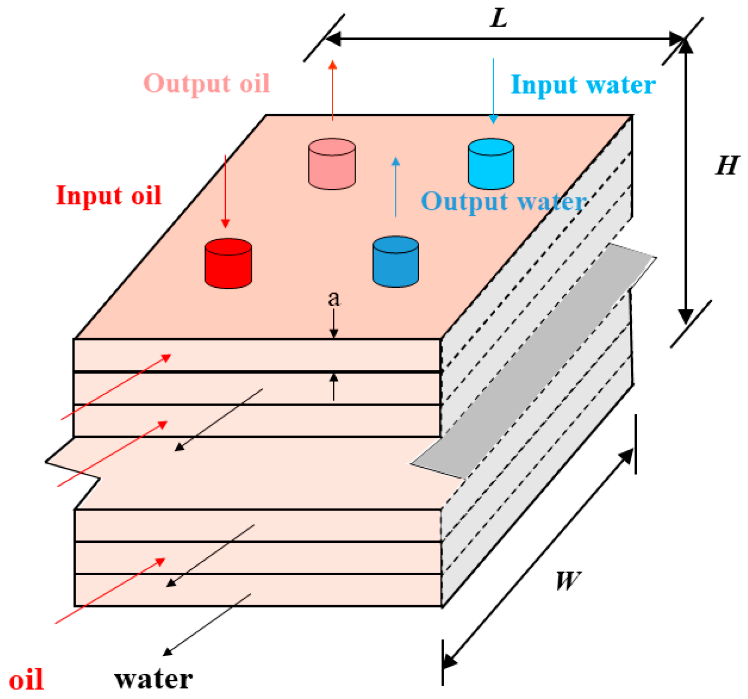
2.3. Thermal Problems and Heat Transfer System

In the heat transfer process with the plate-type heat exchanger shown in Figure 2, the maximum possible heat transfer rate can be expressed as follows [19]:

$$q_{\max }=C_{\min }\left(T_{h,i}-T_{c,i}\right)$$

(8)

where C_min denotes the smaller value between cold fluid heat capacity rate, C_C, and hot fluid heat capacity rate, C_h. T_h,i is the temperature of the inlet hot fluid and T_c,i is the temperature of the inlet cold fluid.

The hot fluid heat capacity rate, C_h, and the cold fluid heat capacity rate, C_C, can be expressed by:

$$\{\begin{array}{c}{C}_h={\dot{m}}_h{c}_{p,h}\\ C_c={\dot{m}}_c{c}_{p,c}\end{array}$$

(9)

The ratio of the actual heat transfer rate for a heat exchanger to the maximum possible heat transfer rate, q_max, can be defined as:

$$\epsilon =\frac{q}{q_{\max }}$$

(10)

where q is the actual heat transfer rate.

The number of transfer units (NTU) is a dimensionless parameter:

$$NTU=\frac{UA}{C_{\min }}=\frac{LW\left(N-1\right)}{C_{\min }\left(1/h_c+1/h_h\right)}$$

(11)

where overall heat transfer coefficient U = (1/h_c + 1/h_h)⁻¹, h_c, and h_h are decided by the cross-sectional area Ac and the wetted perimeter P in ref. [8], and the heat transfer area A = L × W × (N − 1).

After calculating the NTU for the plate-type heat exchanger in our experiment, the effectiveness factor can be derived as follows [30]:

$$\epsilon =2{\left\{1+C_r+{\left(1+C_r\right)}^{1/2}\times \frac{1+\exp \left[-{\left(NTU\right)}_1{\left(1+C_r^2\right)}^{1/2}\right]}{1-\exp \left[-{\left(NTU\right)}_1{\left(1+C_r^2\right)}^{1/2}\right]}\right\}}^{-1}$$

(12)

where C_r = C_min/C_max is the heat capacity ratio.

After calculating Equations (5)–(9), the temperature of the outlet hot and cold fluids can be obtained by:

$$\{\begin{array}{c}{T}_{h,o}=\frac{q}{m_h{c}_{p,h}}+T_{{}_{h,i}}\\ T_{c,o}=\frac{q}{m_c{c}_{p,o}}+T_{c,i}\end{array}$$

(13)

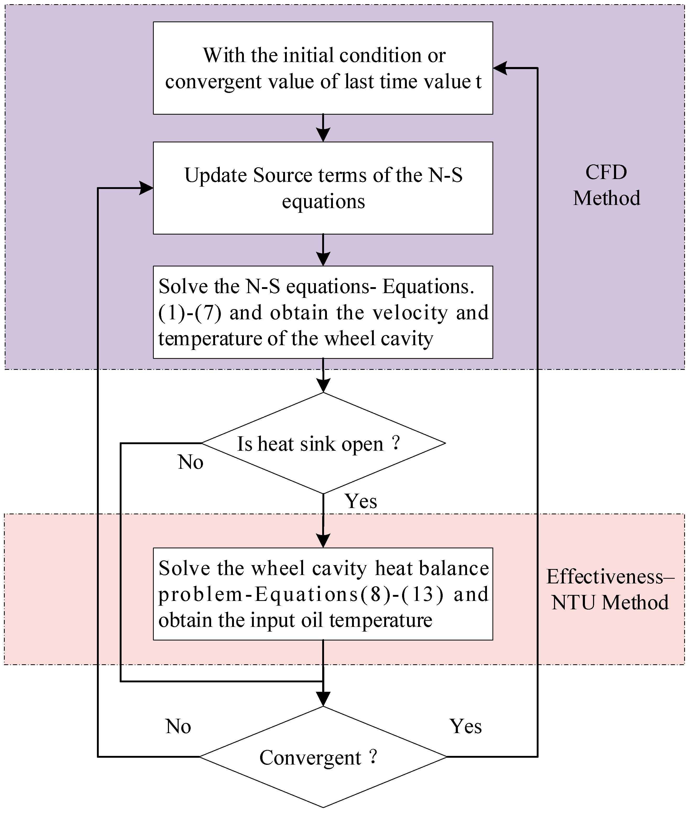
2.4. The Numerical Method

In this paper, a numerical simulation of the hydrodynamic retarder was performed with ANSYS 19.2, where the space-time two-phase flow was solved with a standard k-epsilon turbulence model [31,32,33] and nonequilibrium wall function. This method has been validated in [8,34]. The Frozen Rotor approach [35] was chosen as the interface model, and it ignores the transient effects of the interface to reduce calculation costs while maintaining relatively high computation accuracy. A full flow passage model of the hydrodynamic retarder is shown in Figure 3; for a single flow passage, the outlet spoiler with the inlet ring is where the oil enters and exits. The gas-exhaust spoilers on the stator are set open on the transient oil-filling process and set closed on steady-state simulation. The mesh set can be seen in

Table 1. Node number of mesh.

	Mesh Part	Node Number
Impeller	Rotor	606,780
	Stator	593,125
Flow field	Rotor	142,319
	Stator	108,139
	Inlet part	84,027
	Outlet part	84,959

. To simplify the calculations, the following assumptions are set in the simulation setup: (1) The working medium inside the wheel cavity of the hydrodynamic retarder is set as an incompressible viscous fluid. (2) The influence of the deformation of hydrodynamic retarder components caused by fluid-structure thermal coupling on the flow passage grid is neglected. (3) The density and viscosity of the working medium are determined by the temperature of the wheel cavity, and the influence of temperature on them is shown below. (4) The thermal radiation is not considered in the simulation process, and the heat dissipation effect of the wall is ignored.

To achieve the viscosity–temperature and density–temperature characteristics of the heat transfer medium industrial white oil, the type of white oil is 110#. The viscosity of the white oil is 105–115 mm/s² under 40 °C and 14.3 mm/s² under 100 °C. The density of the white oil is 877 kg/m³ under 15 °C. An experiment was carried out, and the density and viscometers are used to test the viscosity and density under various temperatures with steps of 10 °C. The fitting curve of the viscosity-temperature relationship and density–temperature relationship are shown in Figure 4 and Figure 5. With the curve fitting process, the relationship between dynamic viscosity with temperature and density with temperature can be expressed as follows:

$$\{\begin{array}{c}{f}_{\mu }\left(x_{\mathrm{T}}\right)=0.0000205x_{\mathrm{T}}^2-0.00387x_{\mathrm{T}}+0.19686\\ f_{\rho }\left(x_{\mathrm{T}}\right)=-0.6319x_{\mathrm{T}}+881.45\end{array}$$

(14)

where x_T is the temperature of the white oil.

The calculation process is shown in Figure 6; the effectiveness–NTU method is used to realize the dynamic thermophysical parameter calculation online. To solve Equations (1)–(4), a numerical CFD method was proposed in ANSYS, where the space-time two-phase flow was solved with a standard k-epsilon turbulence model and nonequilibrium wall function; the grid is shown in Figure 3. The Frozen Rotor approach, which ignores the transient effects of the interface to reduce calculation costs while maintaining relatively high computation accuracy, was chosen as the interface model. After the CFD method, the braking torque along with the heat generated can be calculated and interfaced into the Effectiveness–NTU method, which models the heat sink to change the next step’s oil thermal property parameter.

To solve Equations (5)–(11), a heat transfer method is proposed that is integrated into ANSYS software. When the heat sink is set as open, the initial temperature, along with the density and viscosity of the oil in the source term of ANSYS, will be decided by Equations (5)–(11). The input temperature for the CFD method is calculated quickly by a user-defined function in C++ and updates the CFD boundary conditions: mainly the density and viscosity of the white oil. Then, the next step begins to simulate in ANSYS. When the relative error of braking torque is less than 10⁻⁵, that is 0.001%, the method is convergent.

Case 1—Simulation torque considering the influence of temperature on fluid physical properties and fluid kinetic energy

Case 2—Simulation under the isothermal assumption

The two simulation cases were calculated to validate the assumption of variable density and viscosity with the dynamic changing temperature, where Case 1 considers the normal working condition in the oil-filling process.

3. Experiment Set and Validation

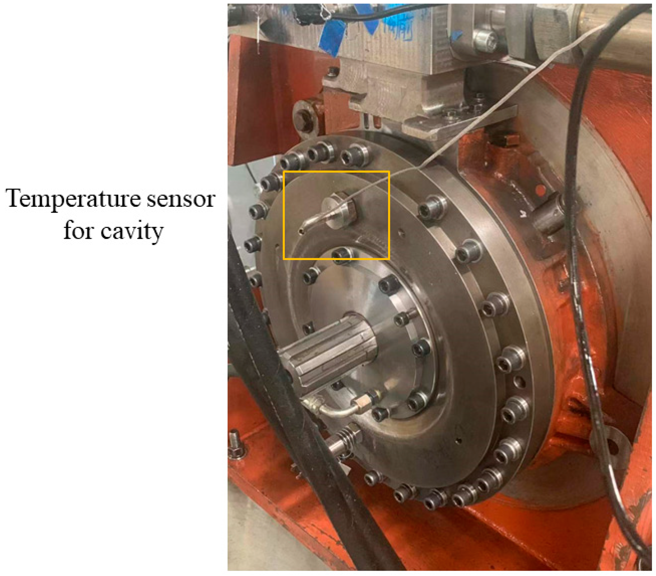
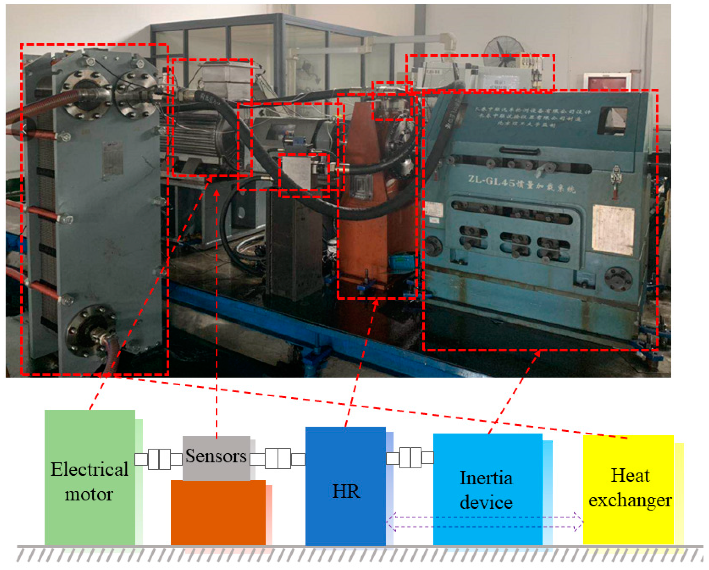
3.1. Experiment Set

The on-site layout of the test bench is shown in Figure 7. The power source (electrical motor) was used to drive the inertia and the hydrodynamic retarder. The rotational speed sensor, torque sensor, and temperature sensor were used to collect the braking torque and temperature of the hydrodynamic retarder.

The test is mainly a torque continuous adjustment test, whose test equipment and arrangement are shown in Figure 8. The bench works under different rotational speeds and studies the maximum braking torque of the hydrodynamic retarder and the changes such as the rotational speed, braking torque, the temperature of the stator, and the inlet and outlet flow when the control current is continuously changed to adjust the opening of the discharge valve. The main measurement speed in steady-state is 800~1100 rpm, each increment is 100 rpm, the control current is 100~400 mA, and each increment is 50 mA.

3.2. Model Validation

Due to the limited driving power of the motor in the experimental environment, the maximum rotor rotational speed is limited to 1100 rpm. To validate whether the temperature has an impact on braking torque and measure the prediction accuracy of the methods with the different assumptions about density and viscosity, Case 1 and Case 2 are compared with the experimental data. The power of the electronic motor shown in Figure 8 is limited; the rotating speed of the experiment is up to 1100 rpm.

In Case 1, the simulated temperature is chosen to meet near the slope of the experiment data, whose slope is shown in

Table 2. Comparisons of experimental and simulation results.

Rotating Speed	Temperature in Experiment	Torque Error Between Case 1 and Experiment	Torque Error Between Case 2 and Experiment
800	144.9	−0.21%	−12.12%
900	144.7	0.92%	−8.12%
1000	134.3	−0.76%	−6.25%
1100	141.6	0.39%	−5.27%

. The results under 140 °C are calculated in Case 1 and are compared with experimental data. Case 2 takes the isothermal assumption and does not consider the effect of temperature on the oil density and viscosity, which keeps a constant value in the simulation. The torque error between Case 1 and Case 2 with experiment data is shown in Table 2. The difference between experimental and simulated braking performance is shown in Figure 9.

In Figure 9, Case 1 covers 60 °C to 140 °C, and to compare with the experiment results, we chose 140 °C as the working condition, which is around the scope of the experiment temperature. Case 2 holds the isothermal assumption that the density and viscosity of the oil are set to be independent of temperature changes. It can be seen in Figure 9 that the calculated braking torques in Case 1 at 140 °C are in good agreement with the experimental data in test rotor rotational conditions (134.3–144.9 °C). As the temperature in the experiment is simultaneously affected by the fluid friction heat generation process and heat sink dissipation process, it is hard to control the experimental temperature at an accurate value such as 140 °C.

As observed from Figure 10, the calculated braking torques in Case 1 are in good agreement with the experiment data in the test rotor rotational condition, with less than 2.5 percent deviations, and the average deviation is approximately 1.13 percent. The average error between Case 2 and the experimental value is 6.478 percent, indicating that the assumption of Case 1 is more in line with the actual heat conduction and dissipation state of the wheel cavity. Thus, the CFD model can be considered valid.

The reason why the experimental torque value is slightly lower than the simulated torque may be the cavitation phenomenon in the high-speed rotation process of rotating machinery [30]. The air in the wheel cavity is difficult to evacuate before the oil-filling process and has difficulties reaching a 100% filling state in the oil-filling process, so the experimental braking torque is slightly lower than the simulation Case 1.

The simulation was carried out on a desktop computer with an Intel Xeon Gold 5120 CPU @ 2.20 GHz. It can be seen in

Table 3. Comparisons of calculation time for Case 1 and Case 2.

Rotating Speed	Calculation Time for Case 1	Calculation Time for Case 2
800	65 min 32 s	64 min 34 s
900	58 min 03 s	59 min 12 s
1000	62 min 46 s	62 min 31 s
1100	61 min 07 s	60 min 57 s

that the calculation time for Case 1 is slightly increased with Case 2, but the calculation accuracy is improved significantly, so Case 1 is more suitable for the simulation of a hydrodynamic retarder when the thermophysical properties are considered.

3.3. Validation for Radiating Circulation Branch

To validate the radiation circulation bench in the hydrodynamic retarder, the comparison of the average temperature in the wheel cavity and braking torque for the test results with a heat sink and without a heat sink in an entire oil-filling process is shown in Figure 11. By controlling the inlet and outlet valve to change the wheel cavity oil-filling rate, the whole adjustment can be divided into four phases according to its rising and steady-state, namely A to D.

In phase A, the oil first enters the inlet passage. It can be observed that the filling rate and the braking torque increase during the filling process in the wheel cavity with and without the heat exchanger. After the liquid filling is completed and the stable phase comes in, the oil temperature in the wheel cavity without a heat sink rises, and the oil temperature in the wheel cavity with a heat sink remains stable.

In phase B, the cooling effect of the newly entered oil on the original oil during the continuous filling makes the temperature curve appear as a downward inflection point. After the filling rate is stable, the wheel cavity temperature increases with time in both cases. It can be seen from the inclination of the curve that the temperature in the wheel cavity rises faster when there is no heat sink than in the case with the heat exchanger.

The above results show that the internal circulation of the heat exchanger efficiently slows down the increase in the oil temperature in the wheel cavity during the braking process of the hydrodynamic retarder, and the braking torque effect is also slightly affected due to the internal circulation of heat dissipation, when the filling rate may not be guaranteed to be consistent.

4. Result and Discussion

4.1. Steady-State Heat Flow Analysis

As shown in Figure 12. The full flow passage model in this paper includes the inter flow passage, the wheel cavity passage, and the outlet flow passage. The temperature cloud map for the full flow passage model is depicted in Figure 12a. The cross section of the flow passage shown in Figure 12b, comprising the velocity vector, above, and the vorticity vector, below, depicts the temperature distribution from the energy dissipation angle.

In the circulation process from the inlet flow passage to the wheel cavity flow passage and then to the outlet flow passage, the oil temperature continuously rises, as depicted in Figure 12a. To interpret this, an analysis of the cross-section of the flow passage is further performed in Figure 12b. Because vorticity is the performance of the fluid viscosity, its size indicates the size of the flow field vortex as well as the degree of energy dissipation caused by secondary flows, such as the vortex. According to the velocity distribution of the oil circulating in the cross-section, when the oil reaches the stator with its speed increasing by the rotation of the rotor, it impacts the blades and the inner surface of the outer ring to reduce its speed. The kinetic energy is converted into internal energy consumption and is dissipated, which can be interpreted from the distribution of vorticity in Figure 12b. There is a large vorticity vector at the impact blade and the inner surface of the outer ring, which causes a local temperature rise.

A full passage analysis of the temperature field and the vorticity field of the rotor region, the stator region, and the interactive region of the rotor and stator will be carried out below.

4.1.1. Rotor

The Cloud diagram of the pressure surface and the suction surface of the rotor in the wheel chamber of the hydrodynamic retarder is shown in Figure 13. The simulation is performed under the condition of a rotational speed of 800 rpm and inlet oil charging speed of 3 m/s. The vorticity distribution and temperature distribution of the pressure surface is shown in Figure 13a,b, respectively, while the vorticity distribution and temperature distribution of the suction surface are shown in Figure 13c,d, respectively. The oil inlet direction along with the oil outlet direction toward the position relative to the cloud map is denoted.

Comparing Figure 13c,d with Figure 13a,b, the distribution trends of the vorticity field and temperature field are the same in pressure surface and suction surface, and the distribution characteristics of the energy dissipation area and the high-temperature area are the same, which is also validated in

Table 4. Comparisons of near-blade flow field under 800 rpm, inlet flow velocity 3 m/s.

Position	Pressure Surface of the Rotor	The Suction Surface of the Rotor	Pressure Surface of the Stator	Suction Surface of the Stator
vorticity (s−1)	368	610.4	317.7	524.8
temperature (°C)	73.85	73.75	73.85	73.85
highest temperature (°C)	75.75	75.85	75.65	75.85

and

Table 5. Comparisons of near-blade flow field under 800 rpm, inlet flow velocity 6 m/s.

Position	Pressure Surface of the Rotor	Suction Surface of the Rotor	Pressure Surface of the Stator	Suction Surface of the Stator
vorticity (s−1)	344.5	580.7	306.8	502.2
temperature (°C)	44.25	44.05	44.25	44.25
highest temperature (°C)	45.65	45.75	45.55	45.65

under the condition of different inlet flow speeds. In particular, in Figure 13a,c, it can be seen that the vorticity near the pressure surface is lower than the vorticity near the suction surface. The difference in the distribution of vorticity reveals the reason why the average temperature near the suction surface is higher than the average temperature near the pressure surface, as shown in Figure 13b,d.

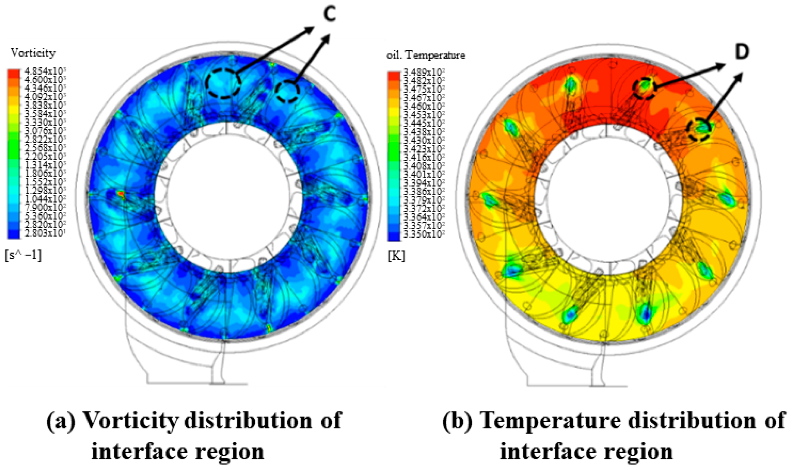
4.1.2. Interface Region

As shown in Figure 14a,b, an analysis of the vorticity field and temperature field of the interactive surface under the rotational speed of 800 rpm and inlet flow rate of 3 m/s is carried out. In Figure 14a, the C area is where the vorticity is larger, and in Figure 14b, the temperature at the corresponding area is lower than the temperature in the edge area. The C area is near the rotor oil inlet passage, which cools the wheel cavity when the oil is input into the wheel cavity, so the temperature in the middle area is lower than the temperature in the edge area.

4.1.3. Stator

It can be seen in Figure 15c that the high vorticity area is concentrated in area D, and from the temperature distribution of area F in Figure 15b, it can be seen that there also exists a temperature concentration phenomenon in the stator that is the same as the rotor. In Figure 15b, it can be seen from the enlarged view of the temperature distribution in the G area that, from the root of the blade to the center of the blade, the temperature of the oil first increases and then decreases. The reason for the increase is that the flow rate of the oil away from the outer ring is high and the energy dissipation is large; the reason for the decrease is the cooling effect of the oil that newly enters the wheel cavity, as mentioned in the interface part.

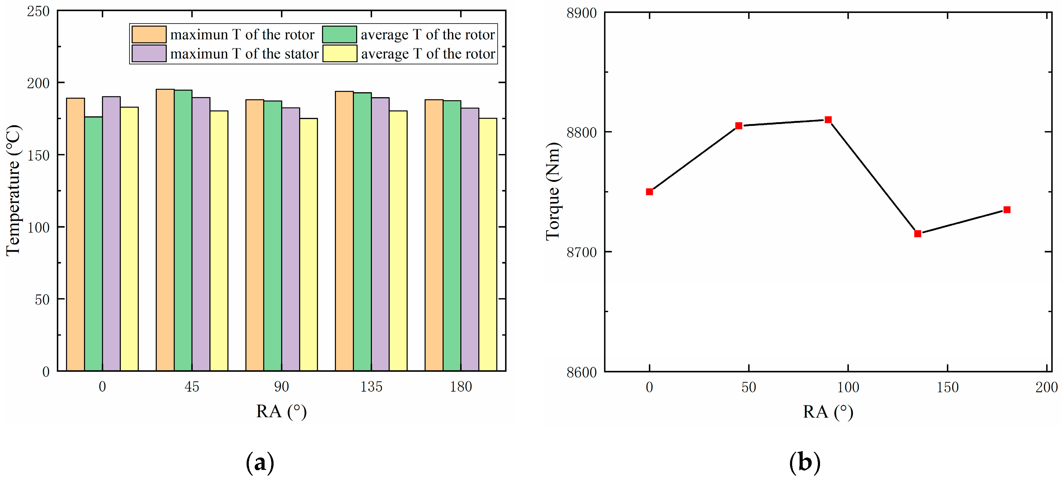
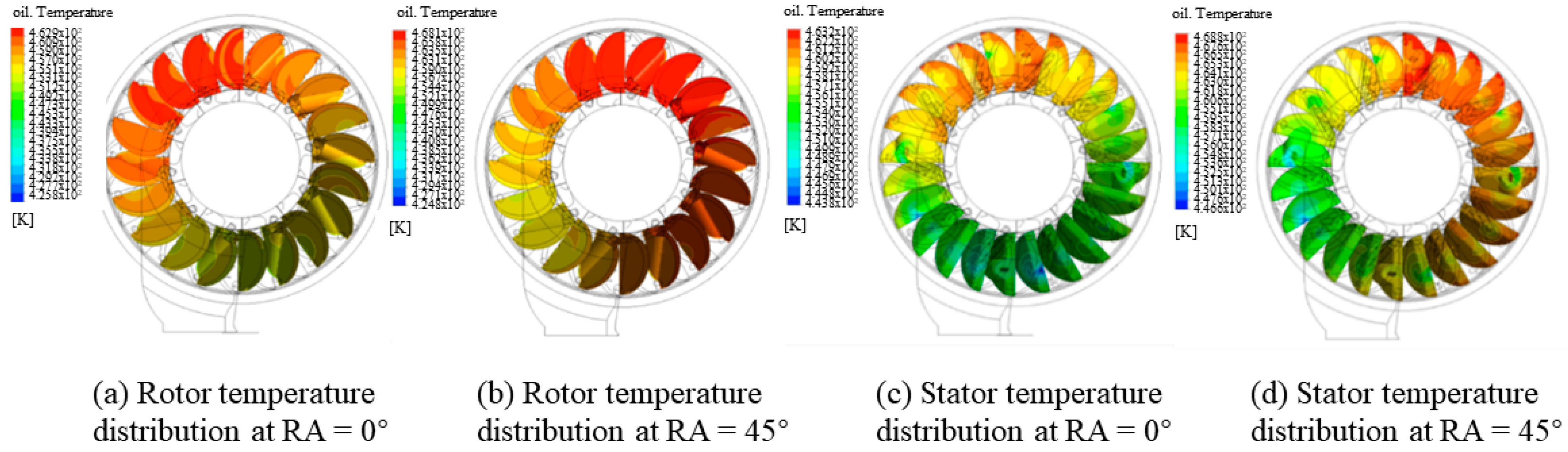
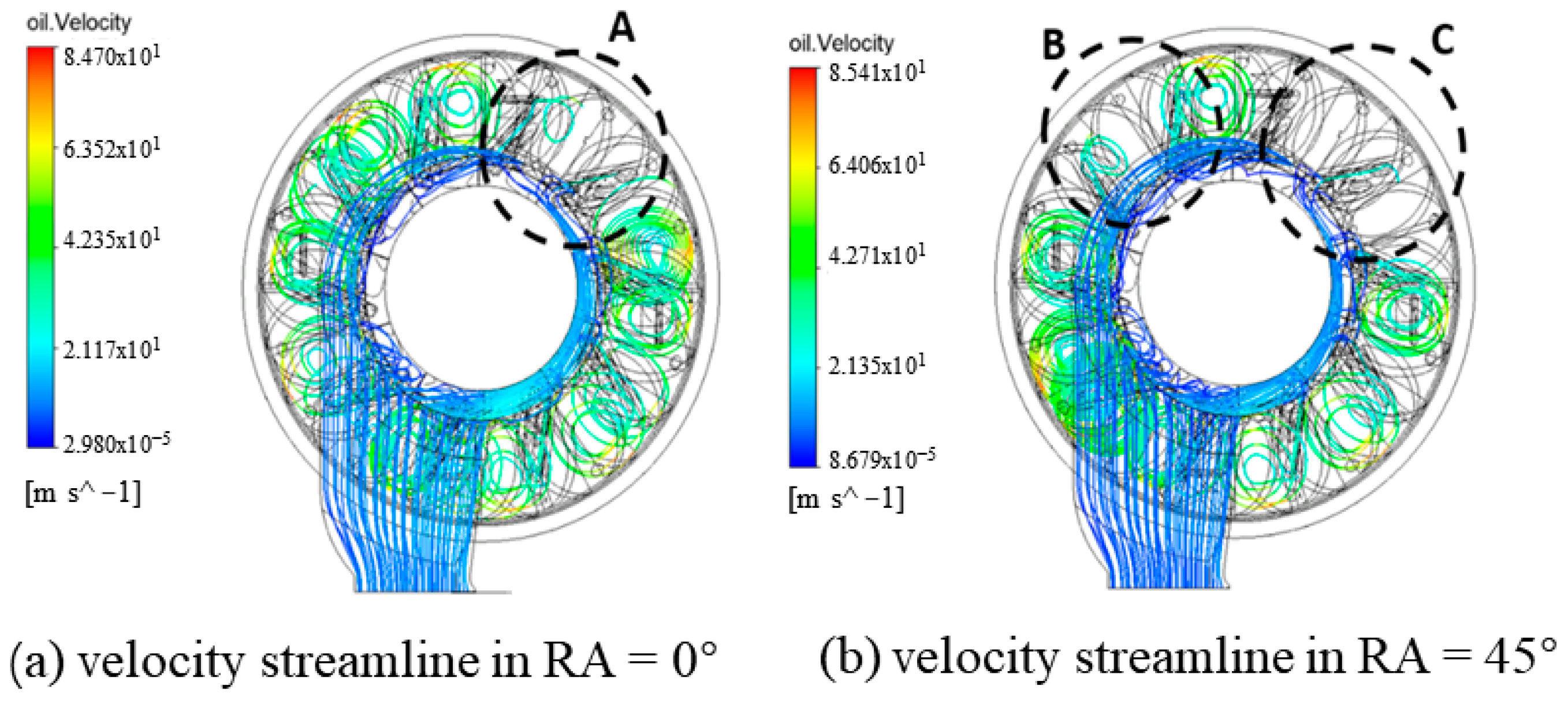
4.2. Effect of Angle of Inlet and Outlet Passages

The steady-state temperature distribution of the hydrodynamic retarder at different speeds is uneven, and there are high-temperature and low-temperature regions. Because the structures of the rotor and the stator of the hydrodynamic retarder are cyclically distributed, the only possible reason for the uneven temperature field distribution of the wheel cavity may be the asymmetric structure of the input and output passages.

To explore the influence of the angle of the input and output passages on the temperature field distribution, the original positions of the input and output passages are set as reference positions, and the position of the input passages is kept unchanged. The angle is changed around the axis of the moving wheel of the hydrodynamic retarder and the Relative Angle (RA) between the position of the output passage and its original position. Considering the symmetry of the rotating machine, the angles of the liquid flow path and the transformation are set as 0°, 45°, 90°, 135°, and 180°, respectively, as shown in Figure 16.

As shown in Figure 17, when the inlet flow rate is the same and the position of the filling passage is given, the different positions of the output passage will have a certain impact on the average temperature and maximum temperature of the wheel cavity. The CFD simulation analysis of the flow field in the hydrodynamic retarder at different angles is carried out, and the temperature field distribution of the wheel cavity, the blade pressure, the braking torque, etc., are obtained with a rotational speed of 1400 rpm and a filling oil speed of 8 m/s. The oil temperature in the wheel cavity of the moving wheel at RA = 45° and RA = 135° is higher than the temperature at RA = 0°, RA = 90°, and RA = 180°, and the stator oil temperature trend is consistent with that of the rotor. For the torque state of each group, the highest torque is achieved at RA = 90°. Comparing the changes in temperature and torque, it can be seen that the degree of torque change with the deflection of the passage has nothing to do with the changing law of the temperature with the deflection.

To learn the effect of the changing passage arrangement on temperature field distribution, in Figure 18 the positions of RA = 0° and RA = 45° are taken as examples to analyze the temperature field distribution. The high-temperature zone is also deflected by a certain angle in the same direction, and both the highest temperature and the average temperature of the wheel cavity have increased, as shown in Figure 18.

To explain the thermal-physics characteristics between different structures, a velocity streamline diagram is used to perform the flow analysis between two classic structures— RA = 0°and RA = 45°. As shown in Figure 19, when the oil enters the wheel cavity from the filling passage of the hydraulic retarder, because the oil itself has a certain initial kinetic energy, the oil does not enter uniformly in the circumferential direction but is affected by the direction of the filling passage. This causes the newly entering oil between the single flow passages in the wheel cavity of the moving wheel to have unevenness. In the RA = 0° structure, the oil in the filling passage enters the wheel cavity relatively uniformly, and only in the A area does less oil newly enter. In the RA = 45° structure, the distribution of the oil in the filling passage is more concentrated in the oil filling process, and there is no new oil in most of the spaces in the B and C areas. Therefore, the cooling effect of the oil newly entering the wheel cavity in the RA = 0° structure is better than that of the RA = 45° structure.

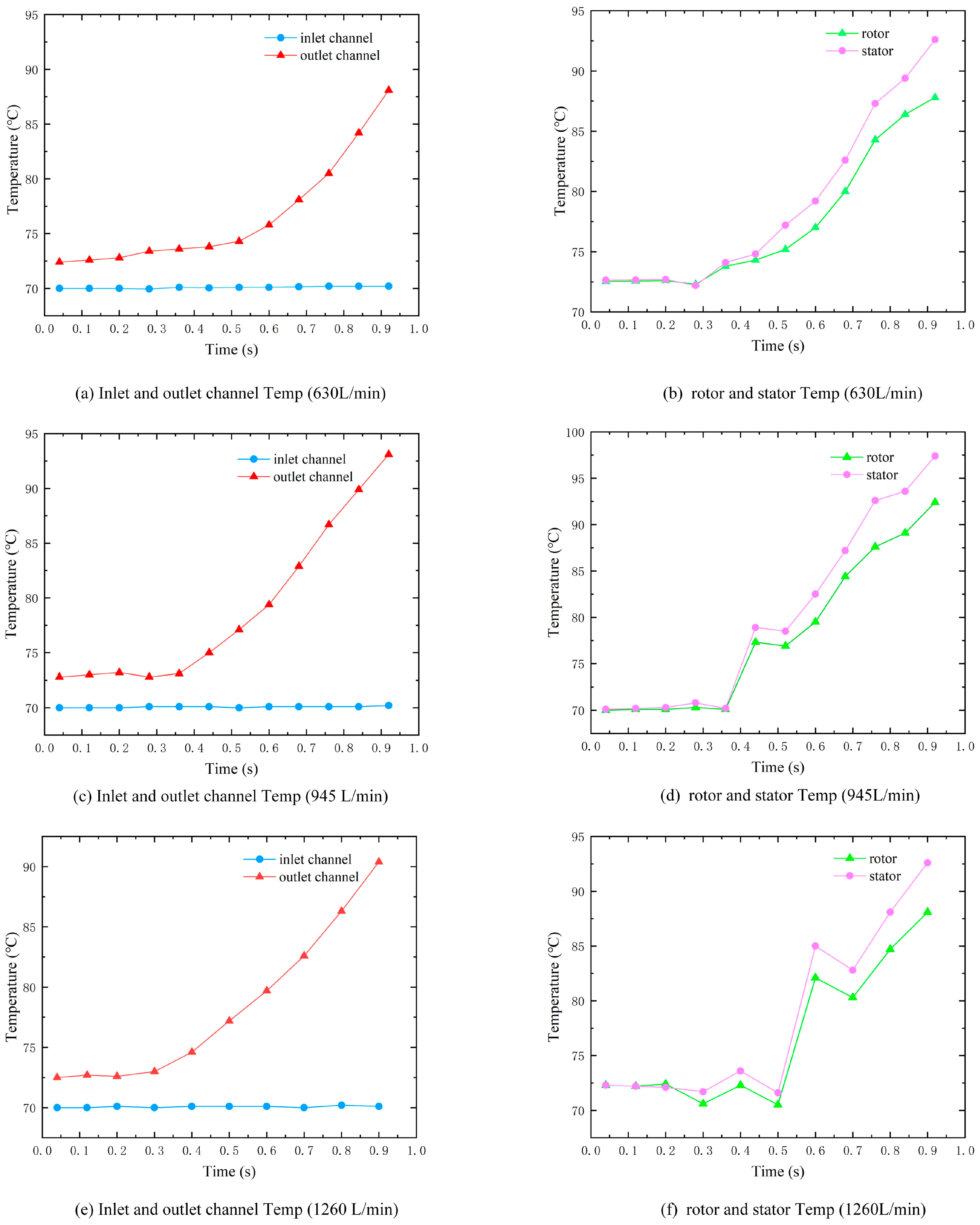
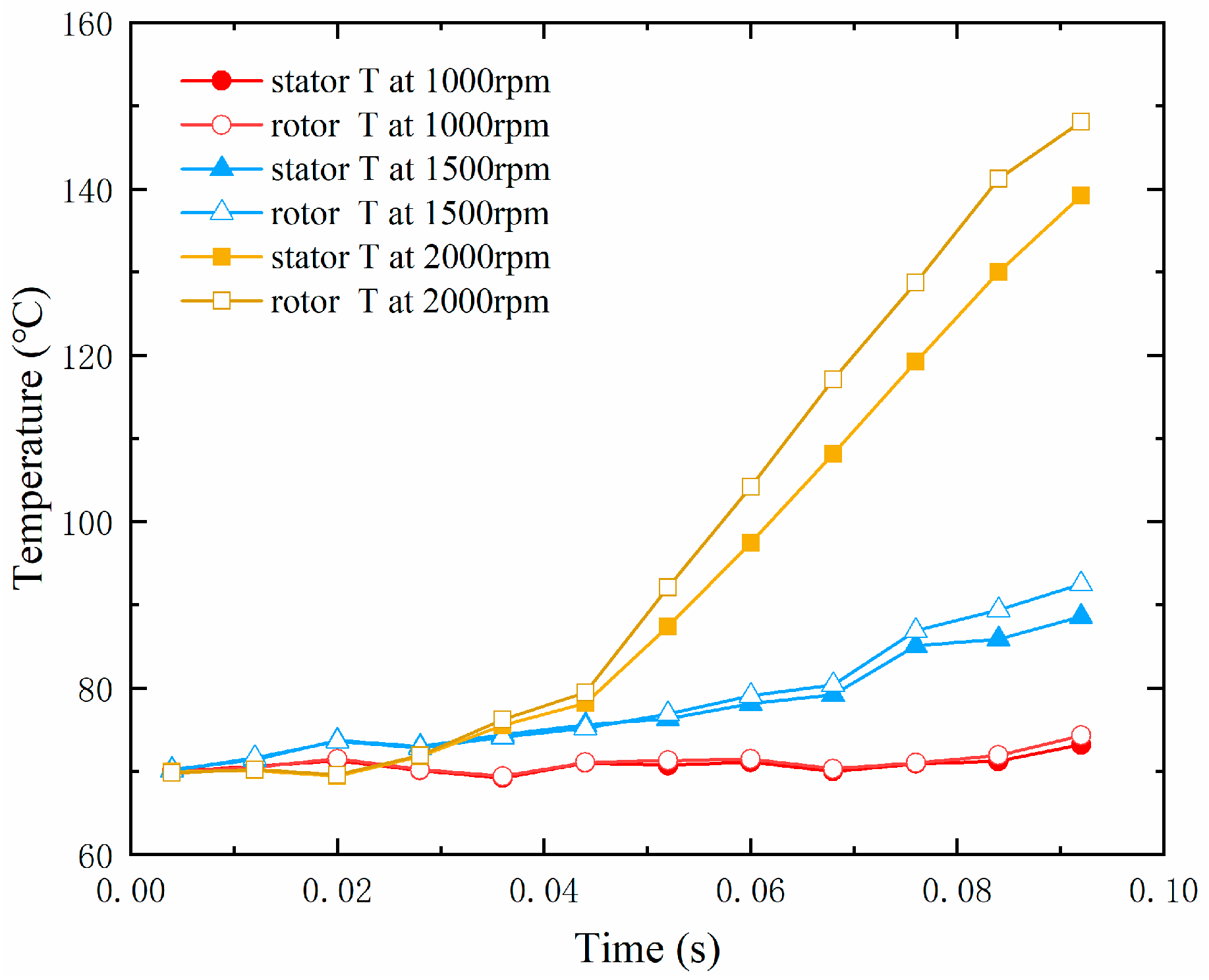
4.3. Effect of Transient Filling Flow and Speed

The transient simulation for an entire oil-filling process is shown in Figure 20. The fluid-filled passage is set as the oil inlet, and the initial temperature of the oil entering the fluid-filled passage is 70 °C. In Figure 20a, the temperature of the oil in the inlet passage has been kept close to 70 °C during the filling process, and the temperature in the outlet passage rises during the filling process. To explain this, it can be seen in Figure 20b that the temperature of the outlet passage and the rotor are close in the initial stage of liquid filling. At this time, the centrifugal force generated by the high-speed rotation of the rotor brings the oil entering the wheel cavity to the outlet passage. There is no energy dissipating component in the outlet passage, so the oil in the outlet passage is not quickly heated. After most of the space in the outlet passage is occupied by oil, the oil that has entered the cavity of the rotor gradually enters the stator.

The stator and the rotor are the main energy-consuming parts of the hydrodynamic retarder, and their energy consumption is mainly formed by hydraulic loss. Both the rotor and the stator are forward-inclined straight blades; the former has 20 blades and the latter has 24 blades. Moreover, the rotor is adjacent to the stator, so the hydraulic loss of them ought to be close. In Figure 20b, the temperature of the oil in the rotor and the stator are not always the same, and the temperature difference observed gradually increases after 0.4 s. The main reason for this is that the moving wheel is directly connected with the inlet passage, so that the oil newly entering the retarder will pass through the rotor first, which has a certain cooling effect on the rotor. The stator and the rotor are connected to each other, and the oil entering the stator from the rotor has a higher initial temperature. In the stator, it interacts with the inner surface of the outer ring of the wheel cavity and the blades to generate secondary energy dissipation. Therefore, during the filling process, the temperature of the stator will be gradually higher than that of the rotor.

In Figure 20c–f, the simulation results of temperature changes in the wheel cavity during the filling process at 945 L/min and 1260 L/min under the rotational speed of 1500 rpm are displayed. Comparing Figure 20b,d,f, the greater the filling flow is, the more tortuous the temperature changes of the rotor and the stator are, which indicates that the filling fluid flow has a certain influence on the temperature distribution in the retarder. At the same time, it can be seen that the larger the filling liquid flow rate, the more obvious is the low-temperature working oil that newly enters the hydrodynamic retarder and cools it.

The temperature-changing state in the wheel cavity during the filling process at different speeds is shown in Figure 21. The temperature difference between the rotor and the stator under 1000 rpm and 1500 rpm is smaller than the difference under 1500 rpm and 2000 rpm. The main reason for this is that, under the same oil charging rate, the torque generated in the hydrodynamic retarder is approximately the quadratic of the speed, so the higher rotational speed led to a higher braking torque, along with the greater temperature rise effect. At the same time, comparing the temperature difference between the rotor and the stator at given rotational speeds, it can be seen that the temperature of the stator will gradually be higher than that of the rotor during the oil filling process, and the temperature difference between the rotor and the stator becomes bigger as the rotational speed increases, which also demonstrates the approximate quadratic relationship between the rotor and the stator.

5. Conclusions

A numerical study of the flow and heat transfer was carried out in a stator–rotor chamber with a plate-type heat exchanger. A CFD tool, combined with a dynamic thermophysical property transfer algorithm, was used to solve the problem. The variable density and viscosity with constant density and viscosity, the method with a heat exchanger, and the method without a heat exchanger were compared on a bench experiment to validate the model accuracy. The distribution of vorticity and temperature in steady simulation was analyzed in the wheel cavity, and the structure-to-performance effect was obtained. The effect of different inlet speeds and rotational speeds was also analyzed in transient oil-filling simulations. Some conclusions of this paper are summarized as follows:

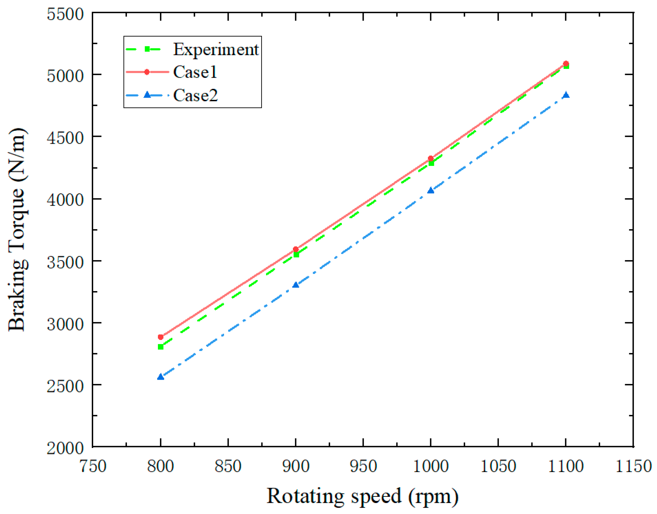
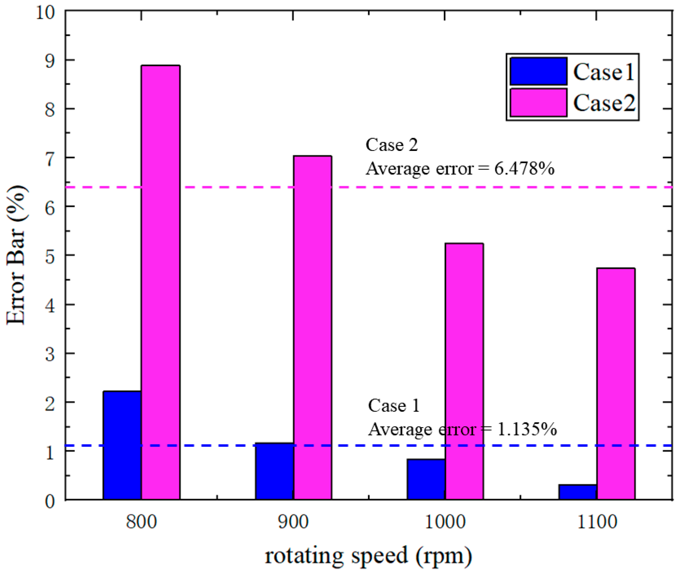
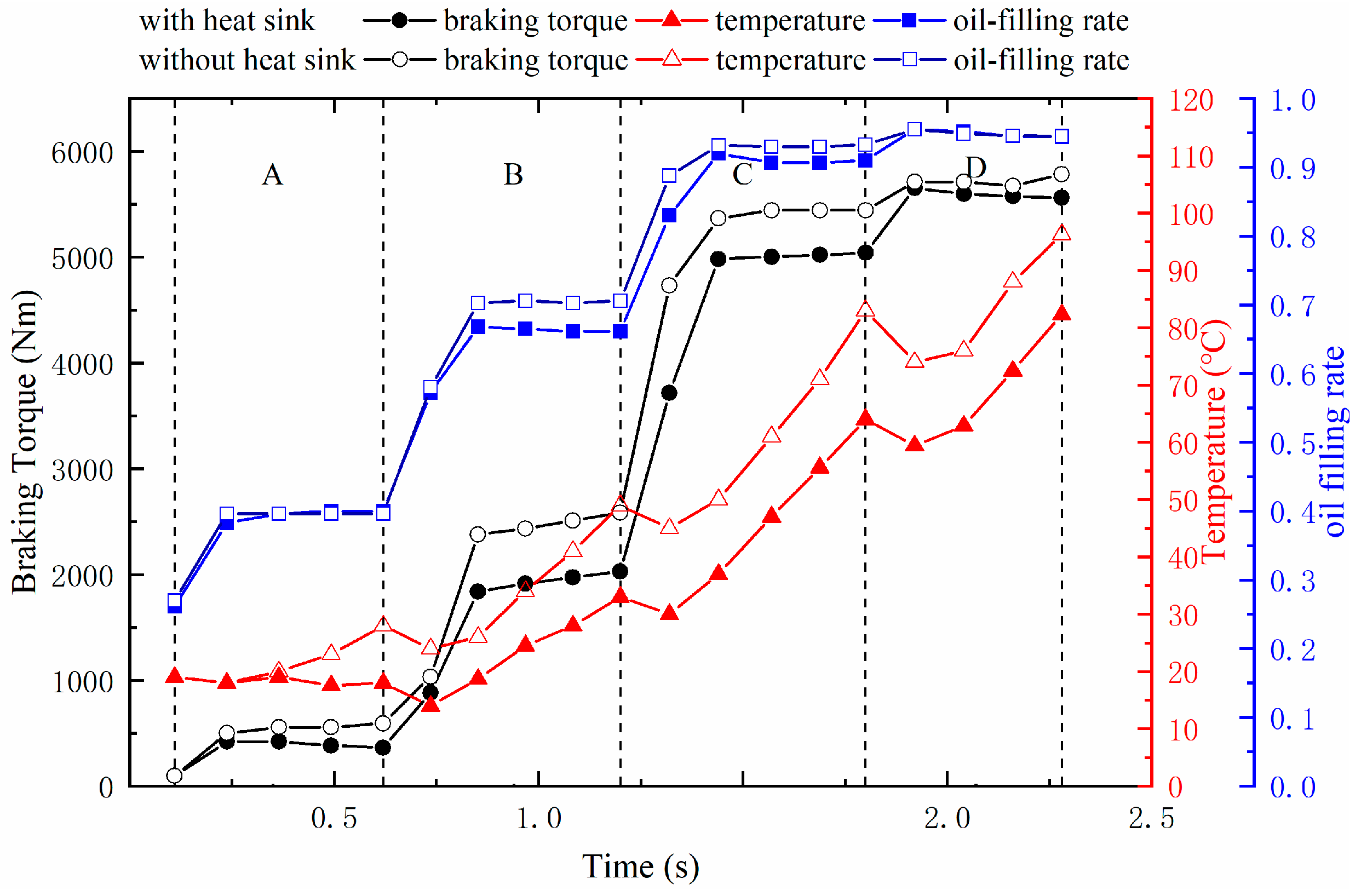
• The numerical results are in good agreement with the experimental data, with a 0.1–2.5% error after considering the variable density and viscosity with the dynamic heat transfer, which is much lower than that of the traditional constant density and viscosity method, the average error of which is 6.478%. The experiment shows that the heat exchanger will efficiently slow down the increase in the oil temperature in the wheel cavity during the braking process of the hydrodynamic retarder.
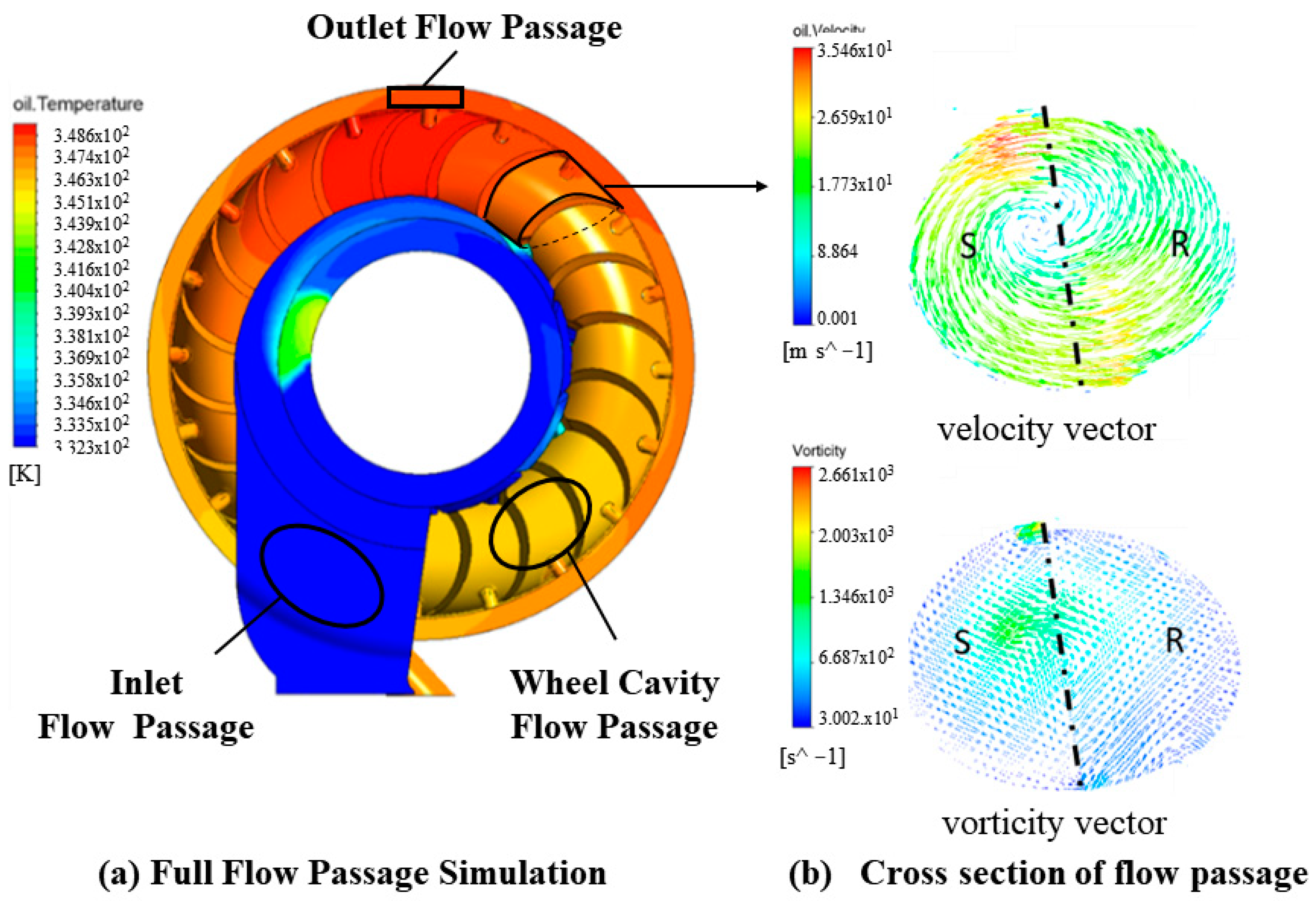
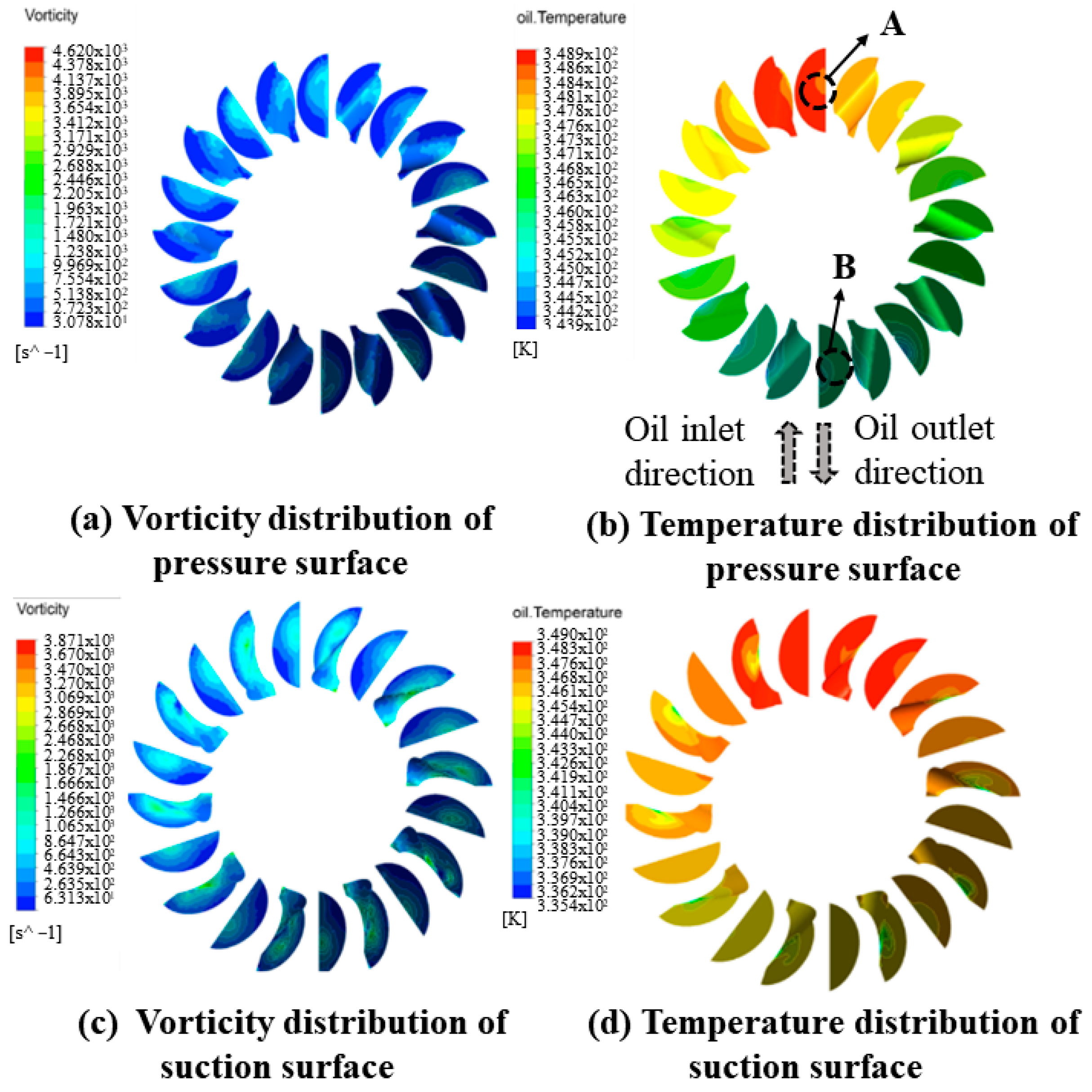
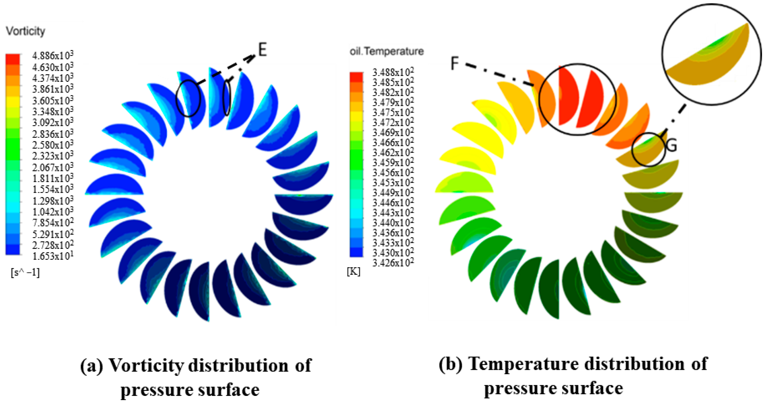
• In steady analysis, the distribution of the energy dissipation area and the distribution characteristics of the high-temperature area are consistent. The temperature distribution of the blades and interface regions is not uniform. The surface temperature of the blades far away from the inlet and outlet is higher than that of the blades near the inlet and outlet for the cooling effect of oil input or output, and there is a high-temperature zone at the rotor blade and the stator blade. Considering the working performance and the average temperature wheel cavity in the working process, the case with 90° for the inlet and outlet passage can provide a larger braking torque while obtaining a better heat dissipation effect.
• A transient simulation analysis of the flow field and temperature field of the wheel cavity of the full flow hydrodynamic retarder was carried out, and the law of the influence of the flow rate and the rotational speed on the liquid filling speed and the brake temperature rise during the continuous torque adjustment process was studied. At the same time during the filling process, the average temperature in the stator is always higher than or equal to the average temperature in the rotor, and it can be seen that the greater the filling flow is, the more tortuous are the temperature changes of the rotor and the stator, while the difference between the average temperature of the rotor and stator increased with rotational speed rise
• The ongoing research will focus on the microscopic flow field of the current model and reflect more detailed thermophysical characteristics by means of Particle Image Velocimetry (PIV) to better visualize the heat-flow coupling phenomenon in cavity chambers.

References

1. Wang, L.; Huang, C.; Hu, J.; Shi, B.; Chai, Z. Effects of temperature-dependent viscosity on natural convection in a porous cavity with a circular cylinder under local thermal non-equilibrium condition. Int. J. Therm. Sci. 2021, 159, 106570. [Google Scholar] [CrossRef]
2. Yan, Q.-D.; Mu, H.-B.; Wei, W.; Liu, S.-C. Design optimization of blade parameters of dual torus hydraulic retarder. Acta Armamentarii 2015, 36, 385. [Google Scholar]
3. Manea, A.; Dobândă, E.; Babic, M. Theoretical and experimental studies on torque converters. Therm. Sci. 2010, 14, 231–245. [Google Scholar] [CrossRef]
4. Mu, H.; Yan, Q.; Wei, W. Study on influence of inlet and outlet flow rates on oil pressures and braking torque in a hydrodynamic retarder. Int. J. Numer. Methods Heat Fluid Flow 2017, 27, 2544–2564. [Google Scholar] [CrossRef]
5. Saqr, K.M.; Aly, H.S.; Kassem, H.I.; Sies, M.M.; Wahid, M.A. Computations of shear driven vortex flow in a cylindrical cavity using a modified k-ε turbulence model. Int. Commun. Heat Mass Transf. 2010, 37, 1072–1077. [Google Scholar] [CrossRef]
6. Zhang, C.; Niu, Y.; Xu, J. An anisotropic turbulence model for predicting heat transfer in a rotating channel. Int. J. Therm. Sci. 2020, 148, 106119. [Google Scholar] [CrossRef]
7. Wang, Z.; Wei, W.; Langari, R.; Zhang, Q.; Yan, Q. A Prediction Model Based on Artificial Neural Network for the Temperature Performance of a Hydrodynamic Retarder in Constant-Torque Braking Process. IEEE Access 2021, 9, 24872–24883. [Google Scholar] [CrossRef]
8. Liu, C.; Xu, N.; Ma, W.; Yuan, Z.; Li, X. Analysis of Unsteady Rotor–Stator Flow with Variable Viscosity Based on Experiments and CFD Simulations. Numer. Heat Transf. Part A Appl. 2015, 68, 1351–1368. [Google Scholar] [CrossRef]
9. Bu, W.; Shen, G.; Qiu, H.; Liu, C. Investigation on the dynamic influence of thermophysical properties of transmission medium on the internal flow field for hydraulic retarder. Int. J. Heat Mass Transf. 2018, 126, 1367–1376. [Google Scholar] [CrossRef]
10. Martin, M.H. The flow of a viscous fluid. I. In Archive for Rational Mechanics and Analysis; Springer: Berlin/Heidelberg, Germany, 1971. [Google Scholar]
11. Naeem, R.K. A class of exact solutions of the Navier-Stokes equations for incompressible fluid of variable viscosity for defined vorticity distribution. Mathematics 2011, 7, 97–118. [Google Scholar]
12. Fatsis, A.; Statharas, J.; Panoutsopoulou, A.; Vlachakis, N. On the exact solution of incompressible viscous flows with variable viscosity. WIT Trans. Eng. Sci. 2012, 74, 481–492. [Google Scholar] [CrossRef]
13. Guo, S.; Sun, L.; Zhang, T.; Yang, W.; Yang, Z. Analysis of viscosity effect on turbine flowmeter performance based on experiments and CFD simulations. Flow Meas. Instrum. 2013, 34, 42–52. [Google Scholar] [CrossRef]
14. Ruan, J.; Wang, X.; Ji, S.; Wang, Y.; An, S. Transient temperature field analysis of variable viscosity RTHSB with a special structural cavity. Adv. Mech. Eng. 2020, 12, 1687814020965051. [Google Scholar] [CrossRef]
15. Mahanti, N.C.; Gaur, P. Effects of varying viscosity and thermal conductivity on steady free convective flow and heat transfer along an isothermal vertical plate in the presence of heat sink. J. Appl. Fluid Mech. 2009, 2, 23–28. [Google Scholar]
16. Arsenyeva, O.; Kapustenko, P.; Tovazhnyanskyy, L.; Khavin, G. The influence of plate corrugations geometry on plate heat exchanger performance in specified process conditions. Energy 2013, 57, 201–207. [Google Scholar] [CrossRef] [Green Version]
17. Luan, Z.-J.; Zhang, G.-M.; Tian, M.-C.; Fan, M.-X. Flow Resistance and Heat Transfer Characteristics of a New-Type Plate Heat Exchanger. J. Hydrodyn. 2008, 20, 524–529. [Google Scholar] [CrossRef]
18. Rohsenow, W.M.; Hartnett, J.P.; Ganic, E.N.; Richardson, P.D. Handbook of Heat Transfer Fundamentals (Second Edition). J. Appl. Mech. 1986, 53, 232–233. [Google Scholar] [CrossRef]
19. Holman, J.P. Heat Transfer; McGraw-Hill Inc.: New York, NY, USA, 2002. [Google Scholar]
20. Guo, Z.; Liu, X.; Tao, W.; Shah, R. Effectiveness–thermal resistance method for heat exchanger design and analysis. Int. J. Heat Mass Transf. 2010, 53, 2877–2884. [Google Scholar] [CrossRef]
21. Bergman, T.L.; Bergman, T.L.; Incropera, F.P.; Dewitt, D.P.; Lavine, A.S. Fundamentals of Heat and Mass Transfer. John Wiley & Sons: Hoboken, NJ, USA, 2011. [Google Scholar]
22. Kays, W.; London, A.J.N.Y. Compact Heat Exchangers; McGraw Hill Book Co.: New York, NY, USA, 1955. [Google Scholar]
23. Uhde, E.; Borgschulte, A.; Salthammer, T. Characterization of the field and laboratory emission cell—FLEC: Flow field and air velocities. Atmos. Environ. 1998, 32, 773–781. [Google Scholar] [CrossRef]
24. Wang, Z.; Zu, S.; Yang, M. Numerical simulation on forced convection over a circular cylinder confined in a sudden expansion channel. Int. Commun. Heat Mass Transf. 2018, 91, 48–56. [Google Scholar] [CrossRef]
25. Li, Y.; Yang, M.; Zhang, Y. Asymmetric phenomenon of flow and mass transfer in symmetric cylindrical and semi-cylindrical shallow chambers. Int. Commun. Heat Mass Transf. 2021, 123, 105174. [Google Scholar] [CrossRef]
26. Pedlosky, J. Geophysical Fluid Dynamics; Springer: Berlin/Heidelberg, Germany, 1987. [Google Scholar]
27. Batchelor, C.K.; Batchelor, G. An Introduction to Fluid Dynamics; Cambridge University Press: Cambridge, UK, 2000. [Google Scholar]
28. Wesseling, P. Principles of Computational Fluid Dynamics; Springer Science & Business Media: Berlin/Heidelberg, Germany, 2001. [Google Scholar] [CrossRef]
29. Olson, L.G.; Bathe, K.-J. Analysis of fluid-structure interactions. a direct symmetric coupled formulation based on the fluid velocity potential. Comput. Struct. 1985, 21, 21–32. [Google Scholar] [CrossRef]
30. Khanlari, A.; Sözen, A.; Variyenli, H.I. Simulation and experimental analysis of heat transfer characteristics in the plate type heat exchangers using TiO2/water nanofluid. J. Numer. Methods Heat Fluid Flow 2018, 29, 1343–1362. [Google Scholar] [CrossRef]
31. Larsson, I.A.S.; Lindmark, E.M.; Lundström, T.S.; Nathan, G.J. Secondary Flow in Semi-Circular Ducts. J. Fluids Eng. 2011, 133, 4491. [Google Scholar] [CrossRef] [Green Version]
32. Launder, B.E.; Spalding, D.B. The Numerical Computation of Turbulent Flows. In Numerical Prediction of Flow, Heat Transfer, Turbulence and Combustion; Elsevier: Amsterdam, The Netherlands, 1983; pp. 96–116. [Google Scholar]
33. Versteeg, H.K.; Malalasekera, W. An Introduction to Computational Fluid Dynamics: The Finite Volume Method; Pearson Education: London, UK, 2007. [Google Scholar]
34. Qian, J.-Y.; Wei, L.; Jin, Z.-J.; Wang, J.-K.; Zhang, H.; Lu, A.-L. CFD analysis on the dynamic flow characteristics of the pilot-control globe valve. Energy Convers. Manag. 2014, 87, 220–226. [Google Scholar] [CrossRef]
35. Dubas, A.J.; Bressloff, N.; Sharkh, S. Numerical modelling of rotor–stator interaction in rim driven thrusters. Ocean Eng. 2015, 106, 281–288. [Google Scholar] [CrossRef]
Figure 1. Schematic diagram of a hydrodynamic retarder.
Machines 10 00887 g001
Figure 2. Diagram of the plate-type heat exchanger; N means the number of types (N = H/a).
Machines 10 00887 g002
Figure 3. Hydrodynamic retarder flow passage model.
Machines 10 00887 g003
Figure 4. Viscosity–temperature of heat transfer medium (white oil).
Machines 10 00887 g004
Figure 5. Density–temperature of heat transfer medium (white oil).
Machines 10 00887 g005
Figure 6. Calculation flowchart.
Machines 10 00887 g006
Figure 7. The stator with the temperature sensor on the test bench.
Machines 10 00887 g007
Figure 8. Test equipment and arrangement.
Machines 10 00887 g008
Figure 9. Comparison between experiment and simulation data of braking torque under 100% charging rate.
Machines 10 00887 g009
Figure 10. Inaccuracy comparison between Case 1 and Case 2 of braking torque.
Machines 10 00887 g010
Figure 11. The change of temperature and braking torque in continuous adjustment conditions under the rotational speed of 1200 rpm.
Machines 10 00887 g011
Figure 12. Temperature field distribution of full flow passages model of hydrodynamic retarder and its interpretation from the vorticity field of the cross-section.
Machines 10 00887 g012
Figure 13. Cloud diagram of the pressure surface and the suction surface of the rotor under the condition of rotational speed 800 rpm and inlet oil charging speed 3 m/s.
Machines 10 00887 g013
Figure 14. Cloud diagram of interface region under the condition of rotational speed 800 rpm and inlet oil charging speed 3 m/s.
Machines 10 00887 g014
Figure 15. Cloud diagram of pressure surface of the stator under the condition of rotational speed 800 rpm and inlet oil charging speed 3 m/s.
Machines 10 00887 g015
Figure 16. CFD models with different relative angles of inlet and outlet passages.
Machines 10 00887 g016
Figure 17. Temperature and braking torque of different relative angles under the rotational speed of 1400 rpm and oil inlet speed of 80 L/min. (a) The maximum and average temperature of the rotor and stator; (b) The external characteristic of the passage. RA = 90° can provide larger braking torque while obtaining a better heat dissipation effect.
Machines 10 00887 g017
Figure 18. Comparison of temperature fields on rotor blades and stator blades at RA = 0° and RA = 45°.
Machines 10 00887 g018
Figure 19. The comparison of velocity streamlines for the structure RA = 0° and RA = 45°.
Machines 10 00887 g019
Figure 20. The temperature change state in the wheel cavity at different filling flow rates at the rotational speed of 1500 rpm.
Machines 10 00887 g020
Figure 21. The average temperature in the wheel cavity under the rotational speed of 1000 rpm, 1500 rpm, and 2000 rpm.
Machines 10 00887 g021