Lightweight Network with Variable Asymmetric Rebalancing Strategy for Small and Imbalanced Fault Diagnosis

Abstract

Deep learning-related technologies have achieved remarkable success in the field of intelligent fault diagnosis. Nevertheless, the traditional intelligent diagnosis methods are often based on the premise of sufficient annotation signals and balanced distribution of classes, and the model structure is so complex that it requires huge computational resources. To this end, a lightweight class imbalanced diagnosis framework based on a depthwise separable Laplace-wavelet convolution network with variable-asymmetric focal loss (DSLWCN-VAFL) is established. Firstly, a branch with few parameters for time-frequency feature extraction is designed by integrating wavelet and depthwise separable convolution. It is combined with the branch of regular convolution that fully learns time-domain features to jointly capture abundant discriminative features from limited samples. Subsequently, a new asymmetric soft-threshold loss, VAFL, is designed, which reasonably rebalances the contributions of distinct samples during the model training. Finally, experiments are conducted on the data of bearing and gearbox, which demonstrate the superiority of the DSLWCN-VAFL algorithm and its lightweight diagnostic framework in handling class imbalanced data.

1. Introduction

With the development of modern industrial technology, the working process of rotating machinery is more integrated and intelligent [1,2,3]. Mechanical components inevitably fail because of the complexity, harshness, and uncertainty of the working environment. The faults that are not detected early can cause serious damage to the equipment and significantly increase the cost of maintenance [4,5]. Therefore, providing effective fault monitoring and health management for mechanical systems plays a crucial role [6].

The response of the defective mechanical parts to the external excitation is abnormal, and thus, the fault signals are generated. The traditional condition monitoring method is to analyze the probability distribution of the signals for fault diagnosis. Such methods are based on artificial feature engineering with a large amount of expert experience, and their capabilities are limited by complex and variable mechanical systems [7,8].

In recent years, deep learning (DL) methods with multi-level nonlinear transformations have been used to autonomously mine information, such as statistical and structural relationships, between data to establish reliable diagnostic models. Consequently, DL methods that can realize the expression of high-dimensional feature information of data have been widely developed. Lei et al. [9] systematically reviewed the development of intelligent diagnosis and provided future prospects. DL methods are continuously improved to solve specific problems. For example, for the problem that samples are disturbed by complex environmental noise in industrial practice, Zhang et al. [10] applied multi-scale feature extraction units to vibration signals for learning complementary and rich fault information on different time scales. Then, a novel easy-to-train module based on adversarial learning was used to improve the feature learning ability and generalization ability of the model. Faced with the problem of variable working conditions, Shao et al. [11] proposed an improved convolutional neural network with transfer learning, which had excellent diagnostic performance in rotor-bearing systems under different working conditions. Therefore, to monitor the invisible faults, Chen et al. [12] exploited the domain-invariant knowledge of the data through adversarial learning between feature extractors and domain classifiers. The fault classifier generalized the knowledge from the source domain to diagnose invisible faults in the meantime. The interpretability of the DL method has also received attention recently. Zhao et al. [13] developed a model-driven deep unrolling approach to realize ante-hoc interpretability, the core of which was to unroll a corresponding optimization algorithm of a predefined model into a neural network, which was naturally interpretable. Additionally, some advanced techniques, such as contrastive self-supervised learning [14], meta-learning [15], metric learning [16] and incremental learning [17], are also utilized by some scholars to solve specific problems in fault diagnosis.

Most existing DL-related methods assume that the distribution of training data is balanced. Nevertheless, the rotating machinery systems often operate in a healthy state, and the collected fault samples only account for a small part. DL models will be dominated by classes with sufficient samples and ignore the minority classes with insufficient feature understanding [18,19,20], which leads to overfitting. If the model is severely biased, resulting in a sharp decrease in the classification accuracy of the minority class, it will influence the maintenance efficiency of the mechanical system. More importantly, it is expensive to collect sufficient annotation signals from industrial equipment. In consequence, it is of great practical significance to correctively classify small and imbalanced data [21,22].

Fault diagnosis methods for small and imbalanced data can be mainly divided into three categories: methods based on sampling technology, data generation and cost-sensitive learning. In general, methods based on sampling techniques are classified as either over-sampling the minority class or under-sampling the majority class [23]. Among them, the synthetic minority over-sampling technique (SMOTE) has yielded many achievements, which augments the data sets by randomly selecting some samples within the nearest neighbor range. Georgios et al. [24] proposed a heuristic over-sampling method based on K-means clustering and SMOTE to generate artificial data, which enabled various classifiers to attain high classification results on class imbalanced data sets. In addition, the adaptive synthetic (ADASYN) over-sampling approach has been used by many researchers to alleviate the degree of class imbalance. Li et al. [25] proposed a fault diagnosis model incorporating ADASYN, a reconstructed data manner and a deep coupled dense convolutional neural network (CDCN), which had satisfactory results on the data set of power transformers. Although resampling methods such as SMOTE and ADASYN have improved the diagnostic performance to a certain extent, the distribution of the sample feature space is difficult to learn due to the complexity of the vibration signals of mechanical equipment, and thereby problems such as distribution marginalization can occur that result in the generation of invalid samples.

With the in-depth study of generative deep learning models, data generation methods represented by generative adversarial networks (GANs) and variational auto-encoders (VAEs) have become the most common means to solve class-imbalanced problems because of their better generated data [23]. VAEs and GANs using unsupervised learning do not aim at extracting features to establish a mapping between input and output but rather learn the distribution of training data and then generate similar data to weaken the impact of class imbalance. Liu et al. [26] proposed a novel data synthesis approach called deep feature enhanced generative adversarial network, where a pull-away function is integrated into the objective function of the generator to improve the stability of the generative adversarial network. This method shows great potential in class-imbalance bearing fault diagnosis. In Ref. [27], an approach based on a conditional variational auto-encoder generative adversarial network (CVAE-GAN) was proposed for imbalanced fault diagnosis. The method utilized an encoder to attain the sample distribution and then generated similar samples by a decoder, and it was optimized continuously through an adversarial learning mechanism. Since the optimization of deep generative models is high-latitude non-convex optimization, such models are usually difficult to train and consume a lot of computational resources, which will miss the optimal time for maintenance during actual fault monitoring. Additionally, if only a few samples are available for training, the real data distribution cannot be fully learned and the quality of the fault samples generated will be too low to meet the requirement of intelligent diagnosis.

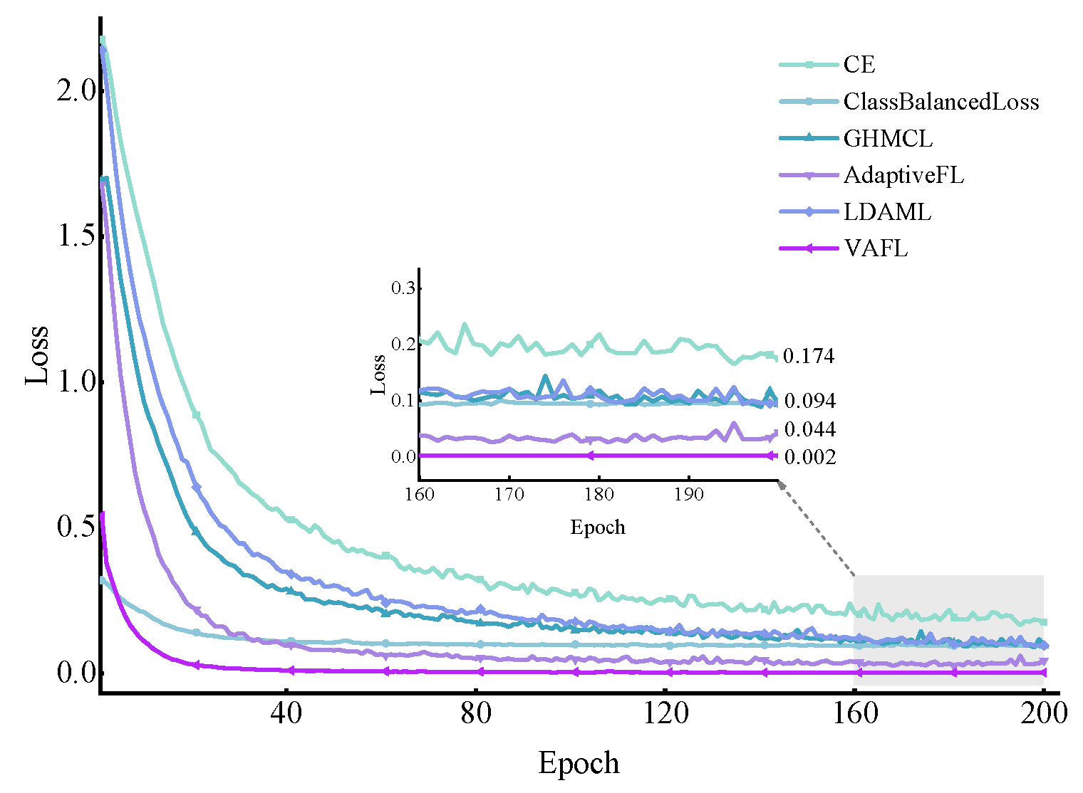
The algorithms based on cost-sensitive learning are dedicated to adjusting the contribution of diverse samples in the model training process by applying cost-sensitive losses [28]. The class-imbalanced problem is solved by imposing cost penalties on distinct classes at the algorithmic level, and such methods are more economical in terms of computational resources and more suitable for establishing lightweight models. Recently, a series of cost loss functions, such as focal loss (FL) [29], class-balanced loss [30], etc., have been proposed to deal with long-tailed distribution data. In the field of fault diagnosis, Geng et al. [31] proposed a new loss function, namely imbalance-weighted cross-entropy (IWCE), which was employed for learning deep residual networks to handle imbalanced bogies fault data from rail transit systems. In Ref. [32], a new CNN-based imbalance diagnosis method was proposed because of the long-tail distribution data from the sensor system. The feature extraction module was optimized by the weighted-center-label loss, while the fault recognition module adopted the distance between the feature and the pattern center vector to diagnose the fault. This manner exhibited effective diagnosis capability for imbalanced data through the automatic extraction of separable and discriminative features. However, many existing cost-sensitive learning methods do not pay attention to the dynamic changes of the corresponding contributions of various samples during the model training. Furthermore, when faced with extremely small samples and serious class imbalance problems, the feature extraction module will fail to fully excavate key features from limited data, which further curbs the effectiveness of cost-sensitive learning methods.

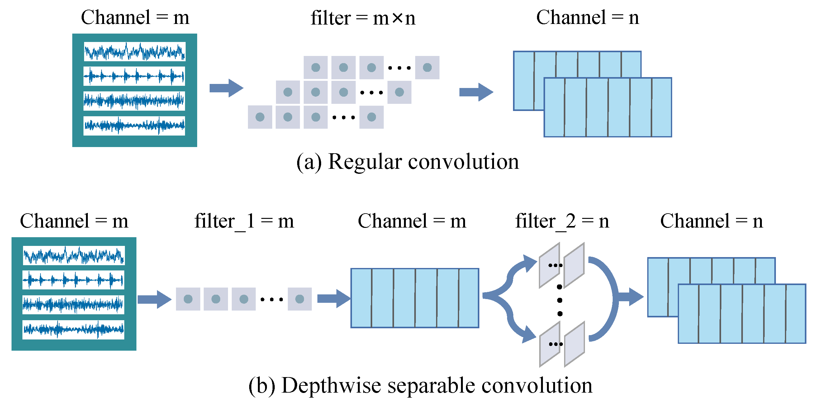
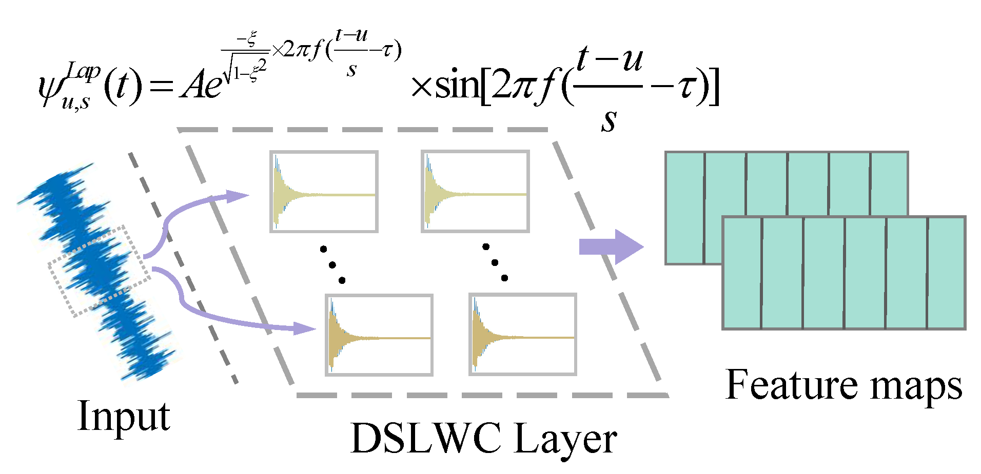
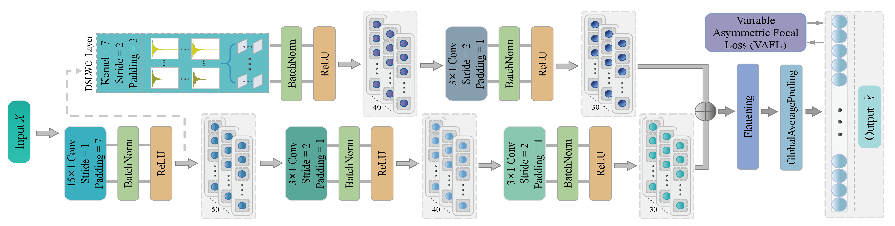
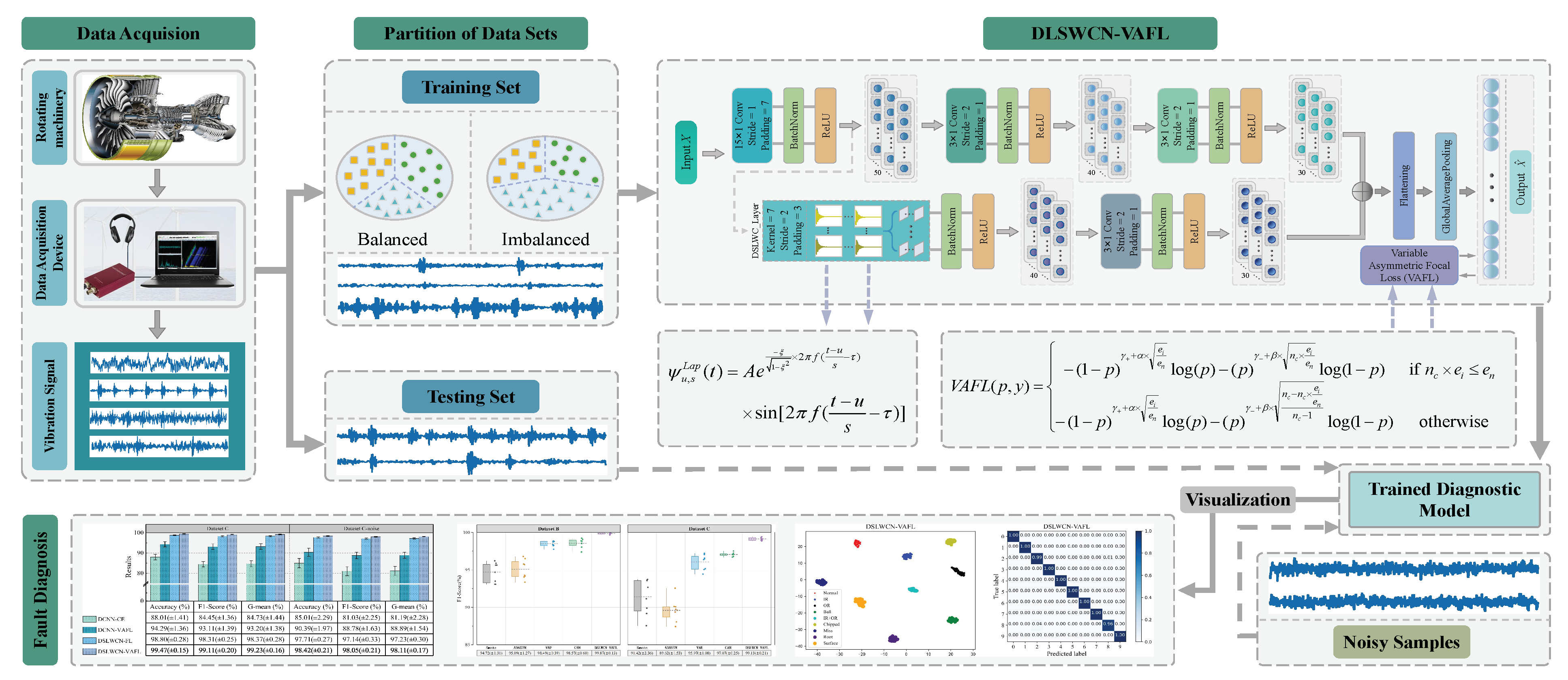
Above all, a lightweight diagnosis framework based on deep separable Laplace-wavelet convolutional network with variable-asymmetric focal loss (DSLWCN-VAFL) is constructed to improve the diagnostic performance in small and imbalanced cases while taking into account the timeliness of faults monitoring. In this method, on the one hand, the multi-scale regular convolutional branch fully learns the time-domain features of the data. On the other hand, the proposed depthwise separable Laplace-wavelet convolution layer containing fewer parameters can excavate the time-frequency features of the data, and then the deeper abstract features are captured by the conventional convolution layer. The combination of these two branches allows for a rich set of discriminative features to be attained from limited samples. In addition, the introduction of global average pooling (GAP) fully retains part of the spatial encoding information of the signals, which not only strengthens the inter-channel connection and reduces the number of parameters but also improves the robustness of the model by increasing the receptive field. Subsequently, a novel asymmetric soft-threshold loss VAFL is designed, which dynamically adjusts the contributions of distinct samples during the convergence of the neural network to alleviate the bias problem of the model. The main contributions of the work are as follows:

1.

A lightweight framework for small and imbalanced fault diagnosis is established, namely DSLWCN-VAFL. This method performs well on extremely small samples and seriously imbalanced class data sets, and it consumes only a small amount of computational resources, whose application prospect is very good.

2.

A new DSLWC branch with few parameters is designed. The branch containing the DSLWC layer can mine the time-frequency features from the input data while increasing few parameters and then cooperate with the multi-scale regular convolutional branch that fully learns the time-domain features so that the model can extract more abundant sensitive feature vectors of different types from the limited signal samples, thereby improving the classification ability.

3.

A novel cost-sensitive loss, VAFL, is proposed. VAFL implements that samples of distinct categories impose a variable cost to highlight the misclassified samples of a minority class, which reasonably rebalances the contributions of diverse samples and alleviates the bias problem caused by imbalanced class data.

4.

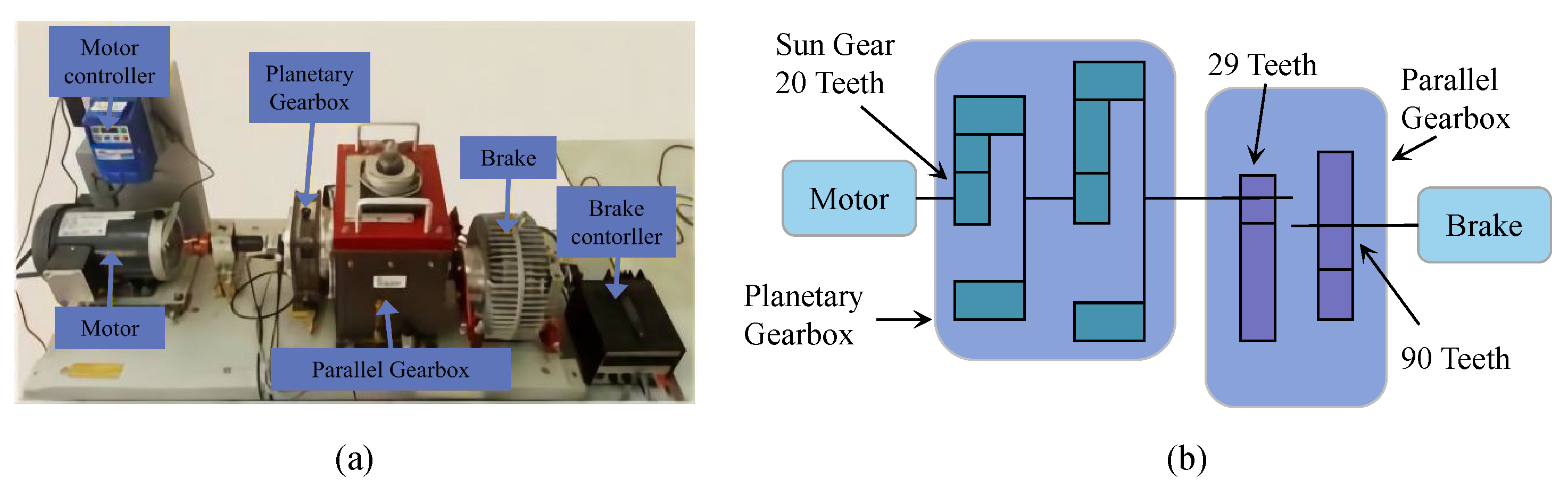
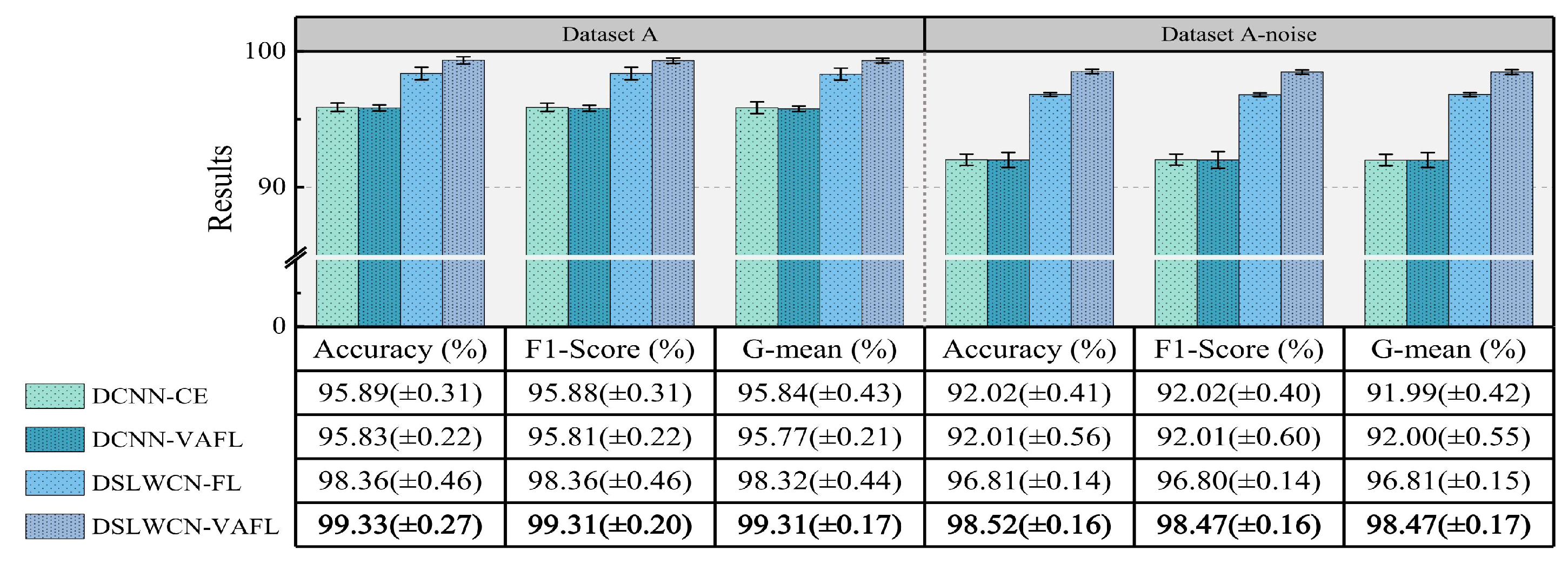
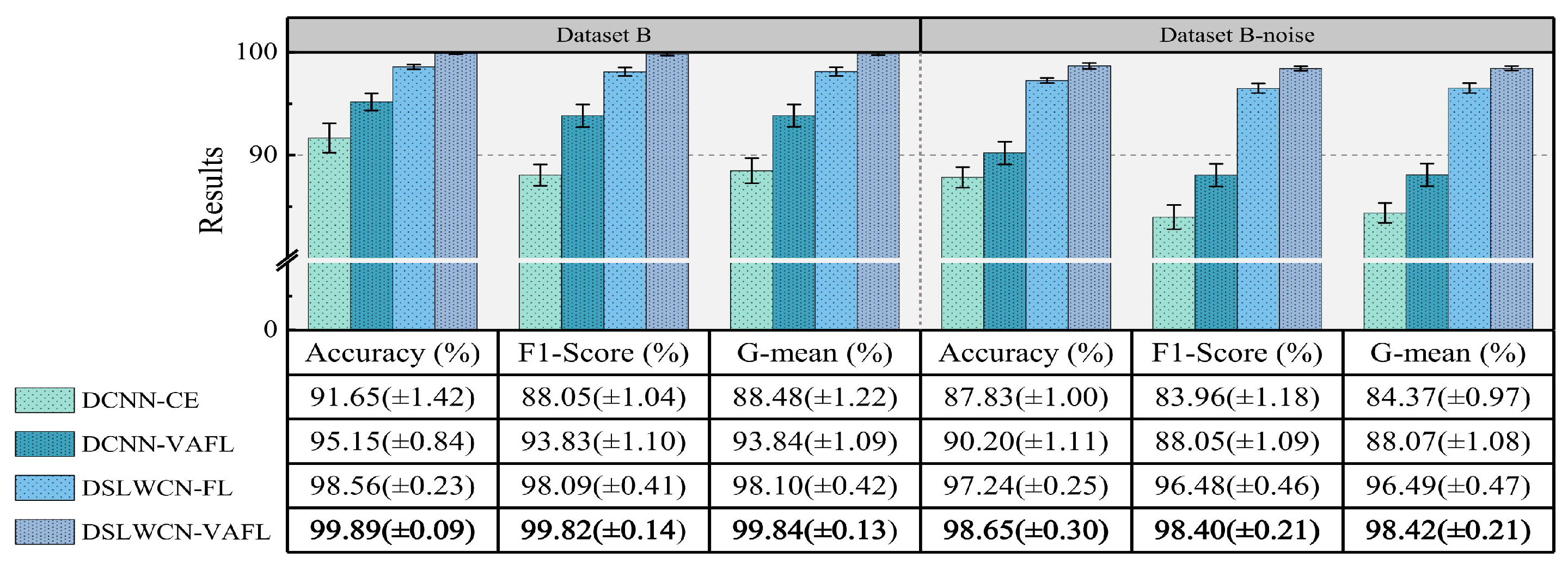
Finally, experiments are conducted on the gear and bearing data sets. The experimental results demonstrate that compared with several popular means, the proposed method achieves an eminent advantage in terms of diagnostic capability and efficiency in the case of limited samples, class imbalance and noisy interference.

The rest of the paper is organized as follows. Section 2 introduces the basic theories briefly. The proposed method is described in detail in Section 3. Section 4 analyzes the proposed method on the gear and bearing signal data sets, respectively. Finally, the conclusion is drawn in Section 5.

2. Background and Related Works

2.1. Depthwise Separable Convolution (DSC)

DSC decomposes the regular convolution into two parts: channel convolution and point-by-point convolution. The difference between depthwise separable convolution and ordinary convolution is shown in Figure 1.

Specifically, the input is expressed as $X\in {\mathbb{R}}^L\times C$, the input channel is C, the output channel is $C^{\prime }$, the size of each filter is $k\times 1$, and the step size is 1. Then, the output can be expressed as $X^{\prime }\in {\mathbb{R}}^{L^{\prime }}\times C^{\prime }$, where $L^{\prime }$ represents the length of the features. In traditional convolution, the input is convolved with C filters to obtain $C^{\prime }$ feature maps. For depthwise separable convolution, an input channel corresponds to one filter to generate C feature maps. In order to achieve $C^{\prime }$ feature maps, $1\times 1$ convolution is introduced to map the previous C feature maps to $C^{\prime }$ feature maps.

The parameters $P_{reg}$ and Floating Point Operations (FLOPs) $F_{reg}$ of the regular convolution are expressed in Equations (1) and (2) [33], respectively.

$$P_{reg}=C^{\prime }\times (C\times k+1)$$

(1)

$$F_{reg}=k\times C\times C^{\prime }\times L$$

(2)

The parameters $P_{sep}$ and FLOPs $F_{sep}$ of the depthwise separable convolution are expressed in Equations (3) and (4), respectively.

$$P_{sep}=C\times k\times 1+C^{\prime }\times (C+1)$$

(3)

$$F_{sep}=(k+C^{\prime })\times C\times L$$

(4)

Therefore, the parameters and FLOPs can be reduced by:

$$\begin{array}{c}\frac{P_{sep}}{P_{reg}}=\frac{C(k+C^{\prime })+C^{\prime }}{C^{\prime }\times (C\times k+1)}\hfill \\ \frac{F_{sep}}{F_{reg}}=\frac{1}{C^{\prime }}+\frac{1}{k}\hfill \end{array}$$

(5)

2.2. Basic Principle of Loss Function

Cross-entropy (CE) loss is a common loss function that measures the difference between the actual probability distribution of samples and the probability distribution predicted by a neural network, which is represented in Equations (6) and (7).

$$p_t=\left\{\begin{array}{cc}p& y=1\\ 1-p& otherwise\end{array}\right.$$

(6)

$$CE(p,y)=-log\left(p_t\right)$$

(7)

where y specifies the truth class and $p\in [0,1]$ is the estimated probability of the network.

However, its effect is not good when dealing with imbalanced problems. Focal loss (FL), as an improved cross-entropy loss, has been proved to alleviate the problem of poor performance of one-stage target detection with extremely imbalanced data [29]:

$$L_{FL}=-{(1-p_t)}^{\gamma }log\left(p_t\right)$$

(8)

where $L_{FL}$ focuses the loss on the low confidence samples. As shown in Figure 2, the closer the probability $p_t$ of the high confidence samples is to 1, the faster the loss weight of the training sample will converge to 0 compared to the cross-entropy.

3. The Proposed Method

3.1. Depthwise Separable Laplace Wavelet Convolution (DSLWC)

When the convolutional layer of a regular CNN performs a set of temporal convolutions between the input data and some finite impulse response filters, the information of key segments cannot be extracted sufficiently by the convolution operation [34]. Moreover, models based on regular convolution operations often suffer from overfitting problems due to the large number of parameters involved.

In order to alleviate the problem above, and inspired by the continuous wavelet convolution kernel [35], the Laplace wavelet is integrated into the convolution kernel, which adds constraints to the convolution kernel waveform to extract explicit periodic pulse information from the input data and fully mine the time-frequency features. In addition, for the purpose of simplifying the structure, the depthwise separable Laplace wavelet convolution layer is proposed to replace the regular convolution layer.

The definition of the basic wavelet dictionary ${\psi }_{u,s}\left(t\right)$ is shown in Equation (9):

$${\psi }_{u,s}\left(t\right)=\psi \left(\frac{t-u}{s}\right)$$

(9)

where $\psi (·)$ is the wavelet basis function, t denotes the time. s is a scale factor, which makes the scaling transform of the wavelet function so that each wavelet traversal approaches different signal frequencies. u is a translational factor so that the wavelet function can traverse the time axis of the signals. s and u are dynamic adaptive adjustable parameters.

Wavelet analysis has a unique advantage in processing nonlinear signals. Mechanical vibration signals belong to non-stationary real signals, so the real Laplace wavelet basis function is adopted, as shown in Equation (10) [36]:

$$\psi \left(t\right)=A{e}^{\frac{-\xi }{\sqrt{1-{\xi }^2}}\times 2\pi f(t-\tau )}\times sin\left[2\pi f(t-\tau )\right]$$

(10)

From Equations (9) and (10), the real Laplace wavelet convolution (LWC) dictionary ${\psi }_{u,s}^{Lap}\left(t\right)$ can be obtained, as shown in Equation (11).

$${\psi }_{u,s}^{Lap}\left(t\right)=A{e}^{\frac{-\xi }{\sqrt{1-{\xi }^2}}\times 2\pi f(\frac{t-u}{s}-\tau )}\times sin\left[2\pi f(\frac{t-u}{s}-\tau )\right]$$

(11)

As shown in Figure 3, DSLWC is further implemented by Equation (11), which is represented in Equation (12):

$$y_{Lap}=\delta [{\psi }_{u,s}^{Lap}\left(t\right)\times x_i]$$

(12)

where $x_i$ is the input feature mapping. $\delta (·)$ is a nonlinear activation function.

The performance of DSLWC is mainly related to the translational factor u and scale factor s. These two dynamic adaptive adjustable parameters are updated by backpropagation, as shown in Equations (13) and (14):

$$\left\{\begin{array}{c}{\ell }_{u_w}=\frac{\partial l}{\partial u_w}=\frac{\partial l}{\partial y_w}\frac{\partial y_w}{\partial {\psi }_{u,s}^w}\frac{\partial {\psi }_{u,s}^w}{\partial u_w}\\ u_{w+1}\leftarrow u_w-\alpha {\ell }_{u_w}\end{array}\right.$$

(13)

$$\left\{\begin{array}{c}{\ell }_{s_w}=\frac{\partial l}{\partial s_w}=\frac{\partial l}{\partial y_w}\frac{\partial y_w}{\partial {\psi }_{u,s}^w}\frac{\partial {\psi }_{u,s}^w}{\partial s_w}\\ s_{w+1}\leftarrow s_w-\alpha {\ell }_{s_w}\end{array}\right.$$

(14)

According to Equations (13) and (14), the gradients of s and u, namely, the composite partial derivation of the loss function, need to be calculated before updating them. ℓ is the gradient, and $\alpha$ denotes the learning rate.

In the calculation process, the partial derivative of the loss function to the feature output $y_w$ is obtained first. Secondly, the partial derivation of $y_w$ to ${\psi }_{u,s}^w$ is gained according to Equation (12). Thirdly, on the basis of Equation (11), the updated gradient ${\ell }_{s_w}$ and ${\ell }_{u_w}$ can be gained, respectively. Finally, a backpropagation is completed by subtracting the product of the learning rate $\alpha$ and the gradient ℓ from the previous value.

In terms of the chain rule and integrating Equations (13) and (14), the gradients of u and s can be calculated as expressed in Equations (15) and (16) to update these two parameters.

$$\begin{array}{c}\frac{\partial {\psi }_{u,s}^{Lap}}{\partial u}=\frac{2\pi Af{e}^{\frac{-\xi }{\sqrt{1-{\xi }^2}}\times 2\pi f(\frac{t-u}{s}-\tau )}}{-s}\times \hfill \\ \left\{\frac{-\xi }{\sqrt{1-{\xi }^2}}sin\left[2\pi f(\frac{t-u}{s}-\tau )\right]+cos\left[2\pi f(\frac{t-u}{s}-\tau )\right]\right\}\hfill \end{array}$$

(15)

$$\begin{array}{c}\frac{\partial {\psi }_{u,s}^{Lap}}{\partial s}=2\pi Af{e}^{\frac{-\xi }{\sqrt{1-{\xi }^2}}\times 2\pi f(\frac{t-u}{s}-\tau )}\times \frac{t-u}{-s^2}\times \hfill \\ \left\{\frac{-\xi }{\sqrt{1-{\xi }^2}}sin\left[2\pi f(\frac{t-u}{s}-\tau )\right]+cos\left[2\pi f(\frac{t-u}{s}-\tau )\right]\right\}\hfill \end{array}$$

(16)

Furthermore, wide convolutional kernels are commonly used for models dealing with 1D-signal data, and although it is easier to understand the low-frequency trend of the input data and thereby suppress the high-frequency noise, more parameters are introduced. In addition, when fine-grained features are abstractly separated from the input data, the number of channels increases significantly to ensure dimensionality reduction without losing information, which will also introduce a large number of parameters and thus affect the computational efficiency of the model. However, the number of parameters in DSLWC is much less than that in regular convolution, which effectively reduces the computational burden. For example, assume that the filter size is $7\times 1$, the input channel is 50, and the output channel is 30. According to Equation (1), the number of parameters of the regular convolution is 10,530. The number of parameters of the depthwise separable convolution is 1880, as calculated by Equation (3). In contrast, DSLWC only needs adaptive adjustment of s, u and the number of parameters required is 1630 $(50\times 2+30\times 51)$, which is only 163/1053 of that in the regular convolution. In summary, the number of parameters required by DSLWC is very small, which can play a huge advantage in establishing lightweight networks.

3.2. Variable-Asymmetric Focal Loss

A sample can be defined as a positive sample if the predicted label of the fault diagnosis model is the same as the true label. At the same time, the samples with estimated probability > 0.5 are easy positive samples, and hard positive samples are those with estimated probability ⩽ 0.5. However, the definitions of easy negative samples and hard negative samples are the opposite of the above. In order to handle the diverse samples from a data set of long-tailed distributions efficiently and pertinently, an asymmetric focal loss function that varies with the epochs is proposed.

Specifically, the role of vanilla focal loss (FL) is to seek trade-offs between the importance of easy and hard samples. When the attenuation factor $\gamma$ is large, FL will inhibit the easy sample. Although the easy samples can be suppressed in this way, the contribution difference between positive and negative samples during the process of the convergence of a neural network is ignored. Therefore, the attenuation factor should be decoupled, and the contribution of positive and negative samples should be rebalanced to help the model update its weight in a better direction. An approach of asymmetric soft-thresholding is employed on the positive and negative parts of the loss to decouple the weighting factors between positive and negative labels, which is represented in Equation (17).

$$\left\{\begin{array}{cc}{L}_{+}=-{(1-p)}^{{\gamma }_{pos}}log\left(p\right)& samples\in Positive\\ L_{-}=-{\left(p\right)}^{{\gamma }_{neg}}log(1-p)& otherwise\end{array}\right.$$

(17)

At the beginning of the training, the deep learning model does not learn the features of the samples well. The percentage of samples that can be classified correctly and have high confidence is not very large. At the same time, the attenuation factor should not be too large for the consideration of reducing the impact on the samples with low confidence. With the advancement of training, the classes (majority) are more easily identified and become easy positive. By increasing the value of the attenuation factor, the dominance of easy positive samples on the loss can be reduced, and thus the weight of the classes (minority) can be increased. Then, for the positive samples, a dynamic positive attenuation factor is proposed, as shown in Equation (18).

$$\begin{array}{cc}{\gamma }_{pos}={\gamma }_{+}+\alpha \times \sqrt{\frac{e_i}{e_n}}& e_i⩽e_n\end{array}$$

(18)

where hyper-parameter ${\gamma }_{+}$ denotes the initial positive attenuation factor. $e_i$ corresponds to the current number of training epochs, and $e_n$ corresponds to the total number of training epochs. The value of ${\gamma }_{pos}$ increases with $\alpha$. In addition, the square root is very sensitive to errors and gives a good indication of the measurement precision of the data, which makes the attenuation factor possess better dynamic adaptability.

For negative samples, the proportion of easy samples will first increase as the features are gradually learned. The easy negative samples dominate the negative part of the loss, which compresses the adjustment of the weights of the hard negative samples that are mainly from the class (minority). Therefore, increasing the value of the attenuation factor can suppress the easy negative samples. However, in the middle and late stages of training, the number of negative samples decreases and the proportion of easy samples also decreases sharply. Accordingly, it is necessary to reduce the attenuation factor to avoid the loss corresponding to the hard samples being too low to weaken the learning ability of the model. For the considerations above, a cyclical negative attenuation factor is proposed for the negative sample, which is expressed in Equation (19).

$${\gamma }_{neg}=\left\{\begin{array}{cc}{\gamma }_{-}+\beta \times \sqrt{n_c\times \frac{e_i}{e_n}}& \mathrm{if}{n}_c\times e_i⩽e_n\\ {\gamma }_{-}+\beta \times \sqrt{\frac{n_c-n_c\times \frac{e_i}{e_n}}{n_c-1}}& \mathrm{otherwise}\end{array}\right.$$

(19)

where hyper-parameters ${\gamma }_{-}$(<${\gamma }_{+}$) denote the initial negative attenuation factor. $\beta$ is the maximum value that ${\gamma }_{neg}$ can increase. $n_c$(⩾1) provides variability for the progress of ${\gamma }_{neg}$ reaching the maximum. ${\gamma }_{neg}$ changes from the minimum to the maximum at $1/\phantom{1n_c}{n}_c$ of the training process and again from the maximum to the minimum for the rest of the epochs. Integrating Equations (18) and (19) with Equation (17), the variable-asymmetric focal loss (VAFL) can be defined as:

$$\begin{array}{c}VAFL(p,y)=\hfill \\ \left\{\begin{array}{cc}\begin{array}{c}-{(1-p)}^{{\gamma }_{+}+\alpha \times \sqrt{\frac{e_i}{e_n}}}\hfill \\ \times log\left(p\right)-{\left(p\right)}^{{\gamma }_{-}+\beta \times \sqrt{n_c\times \frac{e_i}{e_n}}}\times log(1-p)\hfill \end{array}\hfill & \mathrm{if}{n}_c\times e_i⩽e_n\\ \hfill & \\ \begin{array}{c}-{(1-p)}^{{\gamma }_{+}+\alpha \times \sqrt{\frac{e_i}{e_n}}}\hfill \\ \times log\left(p\right)-{\left(p\right)}^{{\gamma }_{-}+\beta \times \sqrt{\frac{n_c-n_c\times \frac{e_i}{e_n}}{n_c-1}}}\times log(1-p)\hfill \end{array}\hfill & \mathrm{otherwise}\end{array}\right.\hfill \end{array}$$

(20)

The discrete value of the sample loss is utilized to locate the boundaries of the easy-hard samples and the positive-negative samples. The contribution rate is then rebalanced according to the different sample losses during the process of backpropagation. Hence, the VAFL function can reasonably adjust the impact of different samples on the convergence process of the model, which is suitable for the intelligent fault diagnosis of class imbalance data.

3.3. The Proposed Framework Based on DSLWCN-VAFL Algorithm

In the fault diagnosis of rotating machinery, it is very expensive and challenging to attain the label fault data of industrial equipment to establish a reliable fault diagnosis structure. Meanwhile, the collected samples of fault conditions are usually far fewer than the samples of normal operation. However, most of the data-driven approaches are based on the premise of a balanced distribution of categories, and the model structure is so complex that it consumes huge computational resources. To this end, a new lightweight model, namely DSLWCN-VAFL for processing class-imbalanced data, is proposed in this paper, as shown in Figure 4. The introduction of the DSLWC layer allows the time-frequency features in the data to be mined and then cooperates with the multi-scale regular convolution branch to fully learn the time-domain features, which enables the model to extract more abundant sensitive feature vectors of different types from the limited signal samples and thus make the data distribution clearer. At the same time, a new cost-sensitive loss mechanism, VAFL, is designed, which reasonably rebalances the contributions of distinct samples during model training.

In industrial applications, the imbalanced fault diagnosis framework based on DSLWCN-VAFL is shown in Figure 5. The specific steps are as follows:

1.

Obtain the vibration signals of the rotating machinery by acceleration sensors.

2.

Perform data segmentation and normalization of the raw vibration signals.

3.

Divide the collected data into training sample set, validation sample set and test sample set.

4.

Input training sample set into DSLWCN-VAFL, and verify the classification performance through the validation set.

5.

Feed the test sample set into the trained DSLWCN-VAFL for fault diagnosis and output the results.

4. Results Analysis and Discussion

4.1. Implementation Details

In order to verify the performance of the proposed imbalanced fault diagnosis method based on DSLWCN-VAFL, various experimental studies will be conducted on the bearing-gear data from Southeastern University and bearing data from Case Western University, respectively. All experiments are implemented in Pytorch 1.8.0, Python 3.8.5, running on AMD Ryzen 7 4800H with Radeon Graphics @2.90 GHz (16G RAM), GTX1650 GPU.

In addition, some specific training parameters are set as follows. The parameter optimizer of the network is Adam, and the learning rate is set to 0.001. According to Refs. [37,38], the batch size is set to 64. An early stop is utilized to avoid overfitting the model. In experiments, some hyperparameters in VAFL have a wide selection range. In general, the attenuation factor is set to 2 [29]. Therefore, the positive attenuation factor ${\gamma }_{+}$ in VAFL is set to 2. While ${\gamma }_{-}$ is less than ${\gamma }_{+}$, ${\gamma }_{-}$ is set to 1. For the consideration of extremely imbalanced situations, such as the number of easy samples is much larger than the number of hard samples, VAFL needs to have a stronger suppression capability. Therefore, the maximum control coefficients $\alpha$ and $\beta$ are set to 3, and the specific structures, parameters, and FLOPs of DSLWCN-VAFL are listed in

Table 1. Detailed network parameters of DSLWCN-VAFL.

No.	Layer Type	Padding	Output	Parameters	FLOPs
0	Input Layer	-	(−1, 1, 1024)	-	-
1	Conv_1D/BN/ReLU	Yes	(−1, 50, 1024)	900	972,812
2	Conv_1D/BN/ReLU	Yes	(−1, 40, 512)	6120	3,150,112
3	Conv_1D/BN/ReLU	Yes	(−1, 30, 256)	3690	952,320
4	DSLWC_layer/BN/ReLU	Yes	(−1, 40, 512)	2120	1,109,596
5	Conv_1D/BN/ReLU	Yes	(−1, 30, 256)	3690	952,320
6	GAP	-	(−1, 30, C)	-	7683
7	Overall parameters			16,520
8	Overall FLOPs				7,144,843

, where the number of classes is expressed as C. According to Refs. [39,40], DSLWCN-VAFL with a small number of parameters and FLOPs can be called a lightweight model, which can effectively reduce the computational burden of fault diagnosis.

When the class-imbalanced data are used for fault diagnosis, even if the samples from the class (majority) are classified wrongly, the accuracy can still maintain a high value through the samples from the class (minority). Therefore, the accuracy is not a good representation of the experimental effect. In addition to accuracy, G-mean and F1-Score are introduced as the evaluation indexes to comprehensively evaluate the classification performance.

$$Accuracy=\frac{TP+TN}{TP+FN+FP+TN}\times 100\%$$

(21)

$$F1-Score=\frac{2TP}{2TP+FP+FN}\times 100\%$$

(22)

$$G-mean=\sqrt{\frac{TP\times TN}{(TP+FN)(TN+FP)}}$$

(23)

where True Positive (TP) is the result of the correct prediction of the positive class. True Negative (TN) represents the result of the correct prediction of the negative class. False Negative (FN) is the result of the incorrect prediction of the negative class. False Positive (FP) denotes the result of the incorrect prediction of the positive class.

4.2. Case 1: Bearing-Gear Data

4.2.1. Data Descriptions

The experimental data are provided by Southeast University [41]. As shown in Figure 6, the steady-state signals are collected from the drivetrain dynamic simulator (DDS) with the rotating speed system load set to 20 HZ-0V. Among them, bearing faults are induced by cracks in disparate locations. The remaining gear faults are divided into four types: Chipped, Miss, Root and Surface. Both Chipped and Root are caused by cracks, while the locations are distinct. The fault Miss is caused by the lack of a gear tooth. Surface indicates the presence of wear on the gear surface. According to Ref. [37], when the number of samples is less than 100, it can be called a small sample problem, and when the number of samples is 10, it is called an extremely small sample problem. During the construction of the data set, scholars hardly set the samples of all classes as limited. In order to fully analyze the performance of the proposed method on small and imbalanced data, three different data sets, A, B and C, are constructed. The specific information is shown in

Table 2. Detailed description of bearing-gear data set.

Data Set	Number of Samples									SNR (dB)
Label	0	1	2	3	4	5	6	7	8
Fault Type	Normal	IR	OR	Ball	IR+OR	Chipped	Miss	Root	Surface
A	10	10	10	10	10	10	10	10	10	None
A-Noise	10	10	10	10	10	10	10	10	10	5
B	100	30	30	30	30	30	30	30	30	None
B-Noise	100	30	30	30	30	30	30	30	30	5
C	100	10	10	10	10	10	10	10	10	None
C-Noise	100	10	10	10	10	10	10	10	10	5

. In the study of class imbalance fault diagnosis, it can be called a seriously imbalanced problem if $N_{fault}/\phantom{N_{fault}{N}_{normal}}{N}_{normal}⩽0.1$, where $N_{fault}$ represents the number of fault samples, and $N_{normal}$ denotes the number of normal samples. It is not difficult to see that the number of samples in data set A is extremely small, the samples in data set B are limited and imbalanced, and the samples in data set C are limited and seriously imbalanced. Each sample contains 1024 sampling points. Moreover, in order to simulate the actual working environment, the Gaussian white noise with SNR = 5 dB is added to each signal to demonstrate the robustness of the proposed model. The raw signals and the noisy signals of the gear fault are shown in Figure 7.

4.2.2. Ablation Experiment

Therefore, to verify the optimization of the performance of DSLWC and VAFL for the network when performing small and imbalanced fault diagnosis, ablation experiments are conducted on the data sets A, B, C and the noisy samples. DSLWCN-VAFL is compared with other models, which are DCNN-CE (without DSLWC and VAFL), DCNN-VAFL (without DSLWC) and DSLWCN-FL (without VAFL). After 200 iteration epochs, the diagnostic performance of the four models on distinct data sets is shown in Figure 8, Figure 9 and Figure 10. In the case where each class is balanced, but the samples are extremely limited, DCNN lacks the ability to extract explicit periodic pulse information from the input data and fully exploit the time-frequency features, and the model complexity does not match the amount of data, which leads to over-sensitivity of the model to noise and outliers and thus overfitting. The lightweight model DSLWCN with few parameters can extract distinct types of multi-scale features to attain more effective features. Therefore, it exhibits an excellent diagnostic performance when dealing with limited samples. From Ref. [28], vanilla FL degrades classification performance when handling balanced data sets. However, the effect of the employment of VAFL is close to CE, which is more suitable for processing balanced data sets.

The diagnostic results of DCNN-CE are disappointing when handling the imbalanced data sets. The main reason is that DCNN itself has poor feature extraction capability and cannot effectively learn features from fault classes with scarce data. More importantly, the cross-entropy loss function does not reasonably balance the contribution of easy-positive and hard-negative samples in the training process of the model, which results in the normal class with sufficient samples dominating the loss and thus failing to implement effective classification. What is worse, the performance of DCNN-CE will decline dramatically as the imbalance problem becomes severe. With the support of VAFL, the imbalance diagnosis performance of DCNN is improved, while DSLWCN with better feature learning capability can also obtain better results with the help of FL. FL balances the contribution of easy and hard samples, which is not realized by CE, and this improves the effect of imbalanced fault diagnosis. However, VAFL that decouples the positive-negative samples and can dynamically adjust the attenuation factor possesses a more reasonable contribution balance strategy, which makes DSLWCN-VAFL gain wonderful diagnostic results even on severely imbalanced data sets. The accuracy, F1-Score and G-mean reach 98.57%, 98.31% and 98.37%, respectively. Through the comparison in Figure 7, it is not difficult to find that the key features used to identify the health of rotating machinery components are easily submerged in the noise, which seriously affects the performance of intelligent fault diagnostic models in practical applications. Nevertheless, DSLWCN-VAFL with detail time-frequency feature extraction ability does not deteriorate substantially when faced with the task of the interference of noises, which indicates that it has a certain anti-noise capability. Moreover, the standard deviation of DSLWCN-VAFL is the smallest compared with others in the comparative experiments, suggesting that it possesses better stability.

Therefore, to further analyze the processing efficiency of the proposed model, the running time of the four models on distinct data sets is listed in

Table 3. Comparison of run time of different models.

Models	Time (s)
Data Set	A	A-Noise	B	B-Noise	C	C-Noise
DCNN-CE	31.29 (±0.21)	31.99 (±0.25)	45.97 (±0.18)	45.62 (±0.36)	39.28 (±0.13)	39.33 (±0.26)
DCNN-VAFL	31.98 (±0.24)	32.84 (±0.35)	48.84 (±0.25)	48.55 (±0.25)	39.54 (±0.14)	39.35 (±0.13)
DSLWCN-FL	27.94 (±0.19)	28.07 (±0.23)	41.97 (±0.19)	42.07 (±0.18)	34.06 (±0.11)	34.01 (±0.13)
DSLWCN-VAFL	26.09 (±0.31)	26.01 (±0.33)	41.89 (±0.20)	42.05 (±0.23)	34.79 (±0.15)	34.79 (±0.16)

. It can not be denied that as a lightweight model, DSLWCN is more advantageous in terms of diagnostic efficiency.

4.2.3. Results of Visualization

For the sake of obtaining a more intuitive feel of the prediction results of different models, visualization tools are introduced. Taking the data set C with severely imbalanced classes and limited samples as an example, the confusion matrix for each model of the first run is plotted. As shown in Figure 11, the overall diagnostic accuracies of the four models are 83.44%, 92.12%, 97.56%, and 98.77%, respectively. It can be found that there is a serious bias in the diagnostic results of DCNN-CE. Nevertheless, after VAFL suppresses a large number of easy-to-classify samples and mines hard-to-classify samples from the classes (minority), the problem of the network deviating to the direction of invalid learning is mitigated, and the updating direction of the gradient is also better optimized. Although the fault signal features corresponding to label 5 and label 6 are relatively difficult to distinguish and lead to misclassification, DSLWCN with stronger feature mining ability can extract different types of multi-scale features from limited samples to improve the fault diagnosis capability.

As another common visualization technique, t-distributed Stochastic Neighbor Embedding (t-SNE) is introduced to verify the diagnostic performance of the proposed method. The data set C is still taken as an example to obtain the feature visualization results after dimensionality reduction in the data. As can be seen from Figure 12, after diagnosis with DCNN, there is an overlap between distinct faults, indicating that faults are not well differentiated. However, DSLWCN makes the spatial distribution differences between various fault classes increase relatively, and the intra-class distribution is relatively dense. Furthermore, the proposed model augmented by the improved rebalancing strategy VAFL makes the distribution boundaries of the classes clearer and enhances the separability, which facilitates the classifier in classifying diverse classes of data and thus improving the monitoring capability of different health states.

4.2.4. Comparison of Various Class Imbalanced Methods

For further analysis of the effectiveness of VAFL, the proposed method is compared with five existing methods. Specifically, CE is the classical technique for class-balanced problems, while the other four are state-of-the-art long-tailed classification techniques: class-balanced loss [30], gradient harmonizing mechanism for classification loss (GHMCL) [42], AdaptiveFocalLoss [43], and label-distribution-aware margin loss (LDAML) [44]. To ensure fairness, the parameters of these methods are set according to the optimal ones in the paper. Experiments are conducted on the three data sets separately, and the diagnostic performance is measured by the F1-Score, as listed in

Table 4. Average F1-Score of various methods.

Loss	F1-Score (%)
	Data Set A	Data Set B	Data Set C
CE	99.42 (±0.08)	95.14 (±0.42)	91.64 (±0.45)
ClassBalancedLoss	98.38 (±0.29)	97.80 (±0.28)	96.54 (±0.32)
GHMCL	98.93 (±0.42)	98.41 (±0.45)	97.18 (±0.63)
AdaptiveFL	99.45 (±0.15)	99.32 (±0.25)	97.96 (±0.17)
LDAML	98.67 (±0.31)	98.84 (±0.34)	96.89 (±0.47)
VAFL(proposed)	99.31 (±0.20)	99.82 (±0.14)	98.31 (±0.18)

. It is undeniable that most long-tailed classification techniques do not perform as well as CE when faced with class-balanced problems, but VAFL does have promising results. Moreover, the F1-Score of the proposed method reaches 99.82% and 98.31% on the moderately imbalanced data set B and severely imbalanced data set C, respectively. Consequently, VAFL also performs well on class-imbalanced data sets. The loss curves of different methods on data set C are plotted in Figure 13. Compared with others, the convergence speed of VAFL is faster, and it can converge in the 25th epoch of the iteration epochs, indicating that it is more computationally efficient. In addition, the fluctuation of VAFL in the later stage is small, and the stability is stronger. All in all, VAFL can replace CE and become a more general technique in the face of either a balanced or imbalanced problem.

4.3. Case 2: Bearing Data

4.3.1. Data Descriptions

The effectiveness of the DSLWCN-VAFL algorithm and its class imbalanced fault diagnosis framework designed in this paper needs to be further explored. Bearing signal data provided by Case Western Reserve University is one of the most widely used standard public data sets in prognostics health management (PHM) [45]. The signal data are gained from the accelerometer of the motor-driven mechanical system. Meanwhile, the sampling frequency is 12 kHz, the motor load is 1hp, the operation is steady-state and the corresponding speed is 1772 r/min. The experimental platform of CWRU is displayed in Figure 14. The experiment simulates three fault states of the bearing: inner ring fault (IR), outer ring fault (OR) and rolling element fault (RE). Additionally, each fault type corresponds to three damage diameters of 0.18, 0.36 and 0.54 mm. Therefore, there are nine fault states: Light Inner Ring fault (LIR), Middle Inner Ring fault (MIR), Serious Inner Ring fault (SIR), Light Outer Ring fault (LOR), Middle Outer Ring fault (MOR), Serious Outer Ring Fault (SOR), Light Rolling Element fault (LRE), Middle Rolling Element fault (MRE) and Serious Rolling Element fault (SRE). The construction of the data sets is still based on a small sample and class imbalanced problem, and the specific information is listed in

Table 5. Detailed description of CWRU bearing data set.

Data Set	Number of Samples										SNR (dB)
Label	0	1	2	3	4	5	6	7	8	9
Fault Type	Normal	LIR	MIR	SIR	LOR	MOR	SOR	LRE	MRE	SRE
A	10	10	10	10	10	10	10	10	10	10	None
A-Noise	10	10	10	10	10	10	10	10	10	10	5
B	100	30	30	30	30	30	30	30	30	30	None
B-Noise	100	30	30	30	30	30	30	30	30	30	5
C	100	10	10	10	10	10	10	10	10	10	None
C-Noise	100	10	10	10	10	10	10	10	10	10	5

. Some bearing signals and noisy signals under different health conditions are plotted in Figure 15.

4.3.2. Diagnosis Results and Analysis

In view of the similar fault diagnosis task, the experimental parameters in Case 2 are kept consistent with those in Case 1. The comparison results of the diagnostic performance of the four models are shown in Figure 16, Figure 17 and Figure 18. Through the comprehensive analysis and verification of the three indicators (Accuracy, F1-Score, G-mean), DSLWCN-VAFL reveals satisfactory diagnostic capability on both class-balanced data sets with extremely limited samples and class-imbalanced data sets. Furthermore, according to the running time of the models in

Table 6. Comparison of run time of different models.

Models	Time (s)
Data Set	A	A-Noise	B	B-Noise	C	C-Noise
DCNN-CE	41.15 (±0.99)	41.09 (±0.52)	69.56 (±0.95)	69.96 (±0.32)	47.02 (±0.57)	46.90 (±0.32)
DCNN-VAFL	41.26 (±0.44)	41.38 (±0.40)	70.29 (±0.18)	70.31 (±0.24)	47.32 (±0.26)	47.32 (±0.27)
DSLWCN-FL	35.80 (±0.43)	35.98 (±0.17)	65.84 (±0.54)	66.02 (±0.18)	40.95 (±0.19)	41.09 (±0.18)
DSLWCN-VAFL	35.53 (±0.35)	35.58 (±0.37)	65.91 (±0.31)	65.80 (±0.23)	39.41 (±0.11)	39.56 (±0.34)

, DSLWCN-VAFL holds excellent diagnostic efficiency as a lightweight class imbalance diagnostic model. In addition, the damage diameter corresponding to the slight fault shown in Figure 15 is smaller, and the features are more blurred under the interference of noise, whereas DSLWCN-VAFL can still achieve an excellent performance of more than 98% in all three indices on severely imbalanced noisy data sets. Taking the data set C with severely imbalanced classes and limited samples as an example, the confusion matrix for each model of the first run is plotted in Figure 19. The overall classification accuracies of the four models are 87.44%, 94.43%, 98.90% and 99.50%, respectively. It can be clearly seen that although the feature extraction ability of DCNN is poor, after the operation of rebalancing the contributions of distinct samples from the class (majority) and class (minority) by VAFL, the probability of the fault class being misclassified as a normal class is greatly reduced. The t-SNE feature visualization of different models in Figure 20 more intuitively highlights that the classification boundary of the features learned by DSLWCN is more clear, and its corresponding 2-D spatial graph shows that the intra-class distribution is more compact and the inter-class distribution is more dispersed. The analysis above, once again, demonstrates that the proposed method has outstanding advantages in class imbalanced fault diagnosis.

4.3.3. Comparison with Other Diagnosis Frameworks

The effectiveness of VAFL and other state-of-the-art classification techniques is further compared on the bearing data sets and measured by the F1-Score, the results of which are presented in

Table 7. Average F1-Score of classification techniques.

Loss	F1-Score (%)
	Data Set A	Data Set B	Data Set C
CE	99.80 (±0.23)	96.06 (±0.35)	93.92 (±1.04)
ClassBalancedLoss	99.33 (±0.37)	98.49 (±0.29)	97.44 (±0.39)
GHMCL	99.47 (±0.40)	98.87 (±0.37)	98.19 (±0.41)
AdaptiveFL	99.84 (±0.15)	99.31 (±0.21)	98.38 (±0.33)
LDAML	99.43 (±0.13)	99.03 (±0.18)	97.83 (±0.34)
VAFL (proposed)	99.88 (±0.11)	99.85 (±0.12)	99.11 (±0.20)

. The diagnostic results of the proposed method are the best and the standard deviation is the smallest, indicating that the stability of DSLWCN-VAFL is excellent.

To verify the superiority of the intelligent fault diagnosis method proposed in this paper, some classical class imbalanced diagnosis frameworks are selected as the comparison frameworks, such as those based on SMOTE [19], ADASYN [46], VAE [47] and GAN [48]. The specific comparison results on two class imbalance data sets with different levels of severity are shown in Figure 21. The results of traditional methods such as Smote and ADASYN on severely imbalanced data sets are dissatisfactory, and the F1-Score only reaches 91.42% and 89.62%. VAEs and GANs have become the most common techniques for solving class imbalanced problems. The new samples generated by such deep learning-related methods based on data synthesis extend the feature space of the original samples, making it easier for the classifier to distinguish diverse types of features, which leads to the advantages of the diagnostic capability of these methods compared to traditional data augmentation methods. However, these deep generative models are often difficult to train and require a lot of computational resources. In contrast, as a lightweight model, DSLWCN-VAFL can still maintain a remarkable diagnostic ability under the premise of consuming limited computational resources, which indicates that its application is promising.

5. Conclusions

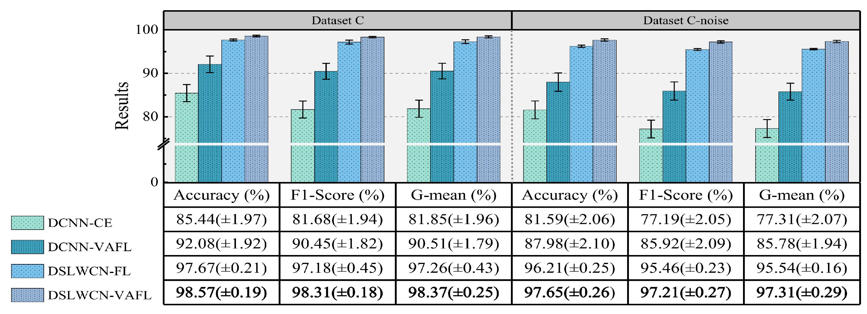
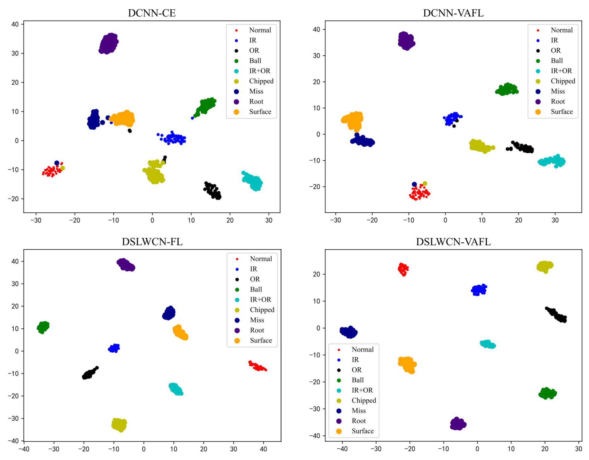
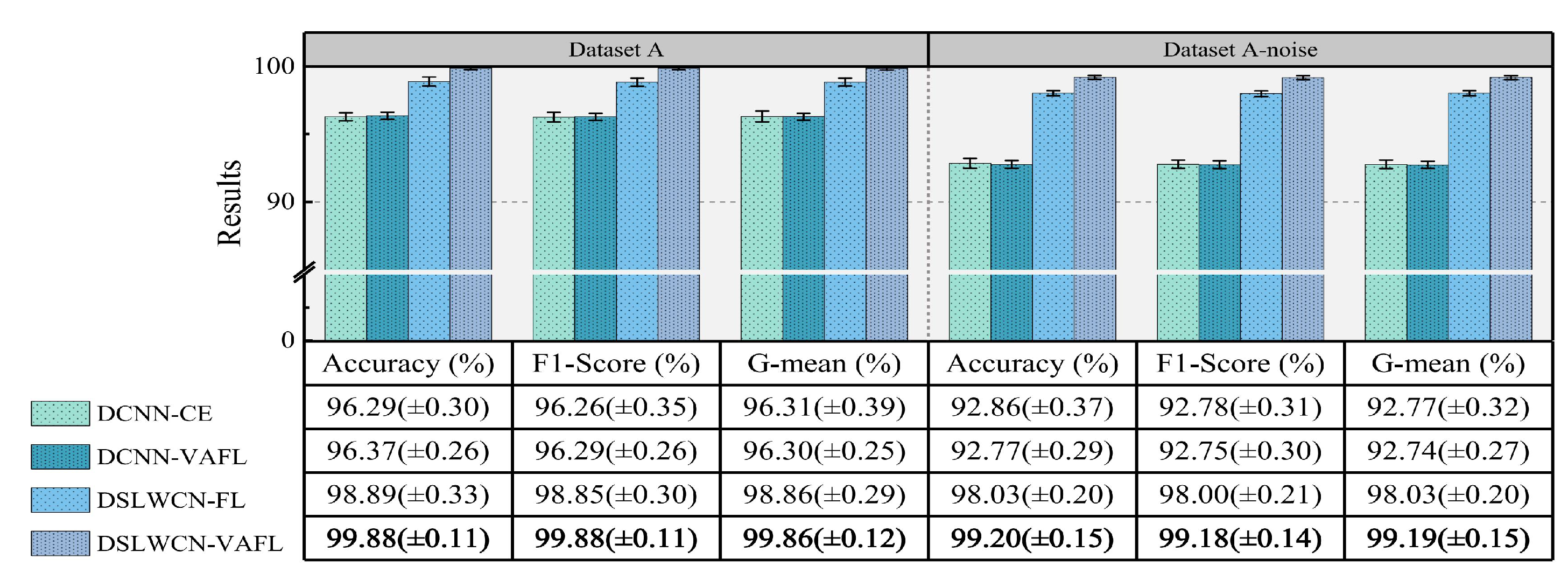
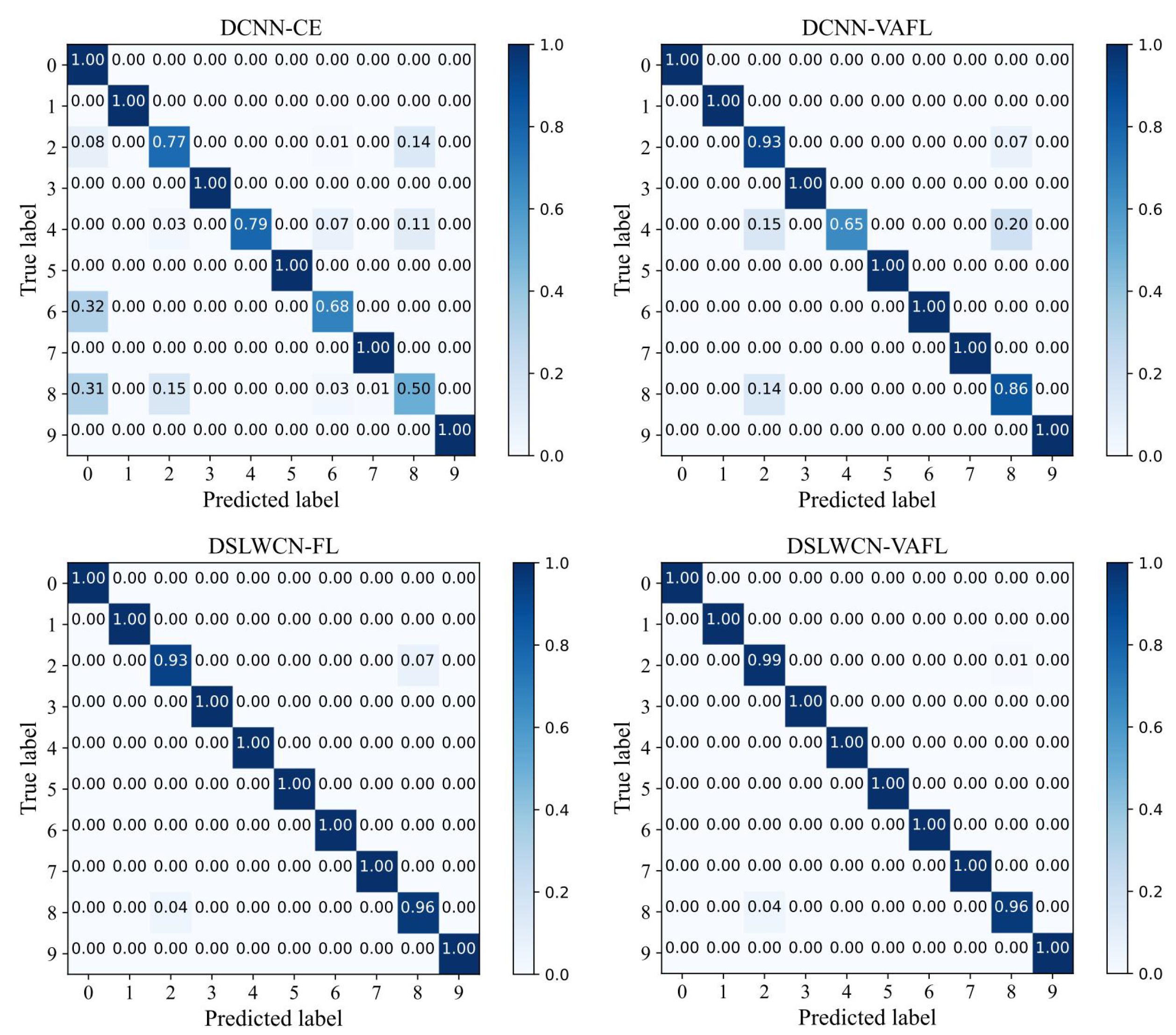
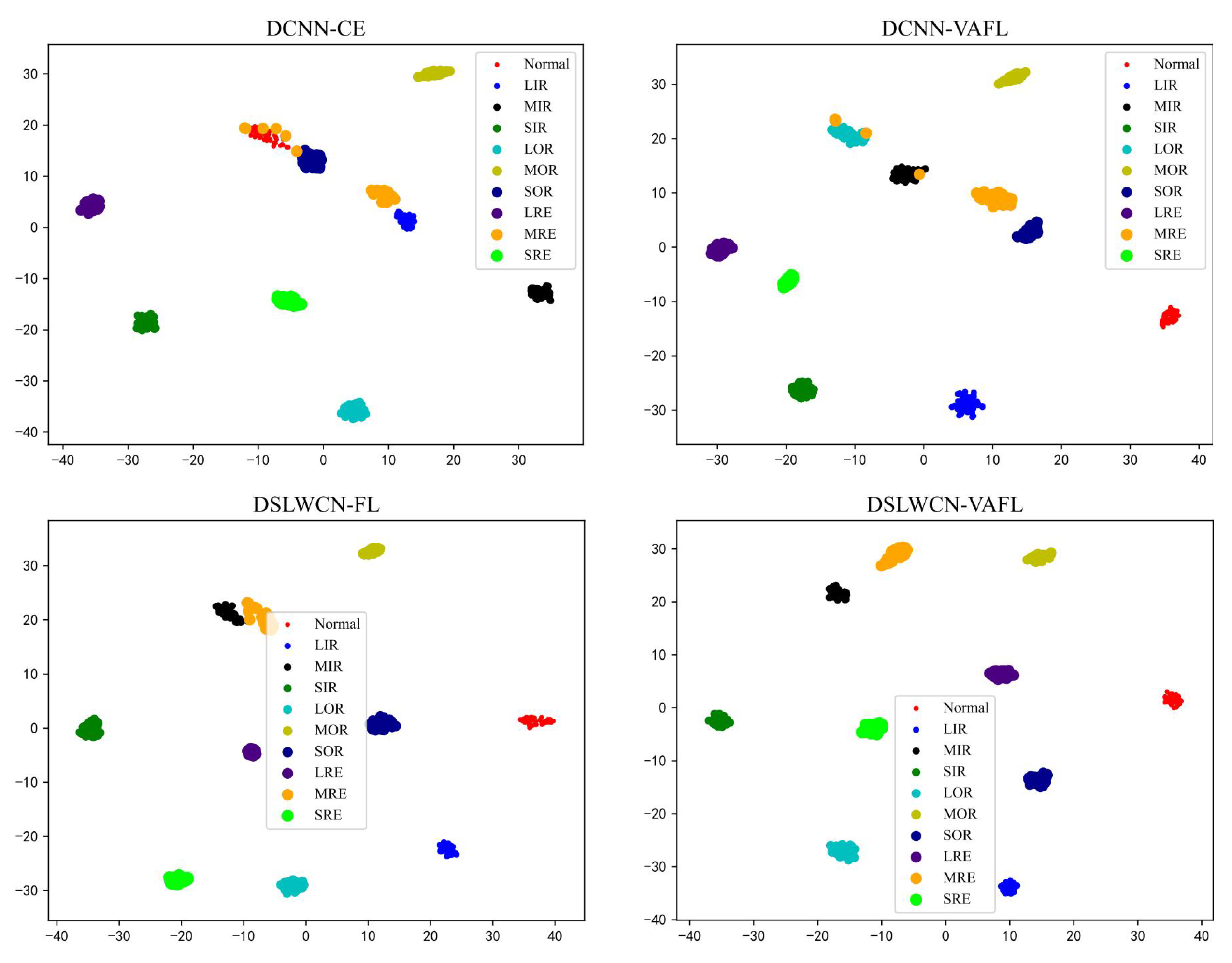
In this paper, a lightweight method named DSLWCN-VAFL is proposed to solve the problem of small and imbalanced data sets. As one of the key technologies in this method, the DSLWC layer not only possesses fewer parameters than regular convolution but also captures time-frequency features from the input 1D data. The branch with the DSLWC layer, combined with the branch of multi-scale regular convolution that can fully learn the time-domain features, achieves abundant discriminative features from limited samples to improve the classification ability of the model. Furthermore, another key technology, namely the novel cost loss VAFL, is designed. The loss function with the ability of dynamic adjustment rebalances the influence of different samples on the convergence of the neural network. Based on the gear and bearing data sets, the diagnostic performance and anti-noise capability of DSLWCN-VAFL in the presence of extremely limited samples and severe class imbalance are discussed in detail. In addition, the effectiveness of each module in the proposed method is verified by ablation experiments. The comparative experiments with some popular methods highlight the superiority of the proposed method. DSLWCN-VAFL not only has promising prospects of application but also provides a new research idea for the solution of class-imbalanced problems.

For future work, the effective processing of multi-source heterogeneous data collected from different sensors is also worth considering, and the noise-insensitive practicability when the data dimension is under strong background noise needs to be further improved. In addition, if faced with variable operating conditions or cross-device diagnosis, it is also worthwhile investigating the employment of techniques such as domain adaptation or transfer learning to solve the imbalanced problem. Finally, the methods for small and imbalanced fault diagnosis through zero-sample learning remain to be explored in extreme cases where no fault samples are available at all.

References

1. Yu, J.; Xiao, C.; Hu, T.; Gao, Y. Selective weighted multi-scale morphological filter for fault feature extraction of rolling bearings. ISA Trans. 2022, in press. [Google Scholar] [CrossRef] [PubMed]
2. Rezazadeh, N.; Ashory, M.-R.; Fallahy, S. Identification of shallow cracks in rotating systems by utilizing convolutional neural networks and persistence spectrum under constant speed condition. J. Mech. Eng. Autom. Control Syst. 2021, 2, 135–147. [Google Scholar] [CrossRef]
3. Rezazadeh, N.; Ashory, M.-R.; Fallahy, S. Classification of a cracked-rotor system during start-up using Deep learning based on convolutional neural networks. Maintenance Reliab. Cond. Monit. 2021, 1, 26–36. [Google Scholar] [CrossRef]
4. Nguyen, V.C.; Hoang, D.T.; Tran, X.T.; Van, M.; Kang, H.J. A bearing fault diagnosis method using multi-branch deep neural network. Machines 2021, 9, 345. [Google Scholar] [CrossRef]
5. Prosvirin, A.E.; Maliuk, A.S.; Kim, J.M. Intelligent rubbing fault identification using multivariate signals and a multivariate one-dimensional convolutional neural network. Expert Syst. Appl. 2022, 198, 116868. [Google Scholar] [CrossRef]
6. Yuan, H.; Wu, N.; Chen, X.; Wang, Y. Fault diagnosis of rolling bearing based on shift invariant sparse feature and optimized support vector machine. Machines 2021, 9, 98. [Google Scholar] [CrossRef]
7. Ren, Y.; Liu, J.; Zhang, H.; Wang, J. TBDA-Net: A Task-based Bias Domain Adaptation Network under Industrial Small Samples. IEEE Trans. Ind. Inf. 2022, 18, 6109–6119. [Google Scholar] [CrossRef]
8. Kumar, V.; Mukherjee, S.; Verma, A.K.; Sarangi, S. An AI-based Non-Parametric Filter Approach for Gearbox Fault Diagnosis. IEEE Trans. Instrum. Meas. 2022, 71, 3516611. [Google Scholar] [CrossRef]
9. Lei, Y.; Yang, B.; Jiang, X.; Jia, F.; Li, N.; Nandi, A.K. Applications of machine learning to machine fault diagnosis: A review and roadmap. Mech. Syst. Sig. Process. 2020, 138, 106587. [Google Scholar] [CrossRef]
10. Zhang, P.; Wen, G.; Dong, S.; Lin, H.; Huang, X.; Tian, X.; Chen, X. A novel multiscale lightweight fault diagnosis model based on the idea of adversarial learning. IEEE Trans. Instrum. Meas. 2021, 70, 3518415. [Google Scholar] [CrossRef]
11. Shao, H.; Xia, M.; Han, G.; Zhang, Y.; Wan, J. Intelligent fault diagnosis of rotor-bearing system under varying working conditions with modified transfer convolutional neural network and thermal images. IEEE Trans. Ind. Inf. 2020, 17, 3488–3496. [Google Scholar] [CrossRef]
12. Chen, L.; Li, Q.; Shen, C.; Zhu, J.; Wang, D.; Xia, M. Adversarial domain-invariant generalization: A generic domain-regressive framework for bearing fault diagnosis under unseen conditions. IEEE Trans. Ind. Inf. 2021, 18, 1790–1800. [Google Scholar] [CrossRef]
13. Zhao, Z.; Li, T.; An, B.; Wang, S.; Ding, B.; Yan, R.; Chen, X. Model-driven deep unrolling: Towards interpretable deep learning against noise attacks for intelligent fault diagnosis. ISA Trans. 2022, 8749–8759. [Google Scholar] [CrossRef] [PubMed]
14. Ding, Y.; Zhuang, J.; Ding, P.; Jia, M. Self-supervised pretraining via contrast learning for intelligent incipient fault detection of bearings. Reliab. Eng. Syst. Saf. 2022, 218, 108126. [Google Scholar] [CrossRef]
15. Long, J.; Zhang, R.; Yang, Z.; Huang, Y.; Liu, Y.; Li, C. Self-Adaptation Graph Attention Network via Meta-Learning for Machinery Fault Diagnosis With Few Labeled Data. IEEE Trans. Instrum. Meas. 2022, 71, 3515411. [Google Scholar] [CrossRef]
16. Huang, K.; Wu, S.; Sun, B.; Yang, C.; Gui, W. Metric Learning-Based Fault Diagnosis and Anomaly Detection for Industrial Data With Intraclass Variance. IEEE Trans. Neural Netw. Learn. Syst. 2022, 1–12. [Google Scholar] [CrossRef] [PubMed]
17. Zhou, H.; Yin, H.; Zhao, D.; Cai, L. Incremental Learning and Conditional Drift Adaptation for Non-Stationary Industrial Process Fault Diagnosis. IEEE Trans. Ind. Inf. 2022, 1. [Google Scholar] [CrossRef]
18. Gao, Y.; Gao, L.; Li, X.; Cao, S. A Hierarchical Training-Convolutional Neural Network for Imbalanced Fault Diagnosis in Complex Equipment. IEEE Trans. Ind. Inf. 2022, 18, 8138–8145. [Google Scholar] [CrossRef]
19. Jalayer, M.; Kaboli, A.; Orsenigo, C.; Vercellis, C. Fault Detection and Diagnosis with Imbalanced and Noisy Data: A Hybrid Framework for Rotating Machinery. Machines 2022, 10, 237. [Google Scholar] [CrossRef]
20. Li, B.; Tang, B.; Deng, L.; Wei, J. Joint attention feature transfer network for gearbox fault diagnosis with imbalanced data. Mech. Syst. Sig. Process. 2022, 176, 109146. [Google Scholar] [CrossRef]
21. Ganaie, M.A.; Tanveer, M.; Alzheimer’s Disease Neuroimaging Initiative. KNN weighted reduced universum twin SVM for class imbalance learning. Knowl.-Based Syst. 2022, 245, 108578. [Google Scholar] [CrossRef]
22. Rezazadeh, N.; De Luca, A.; Perfetto, D. Unbalanced, cracked, and misaligned rotating machines: A comparison between classification procedures throughout the steady-state operation. J. Braz. Soc. Mech. Sci. Eng. 2022, 44, 450. [Google Scholar] [CrossRef]
23. Zhang, T.; Chen, J.; Li, K.; Lv, H.; He, S.; Xu, E. Intelligent fault diagnosis of machines with small & imbalanced data: A state-of-the-art review and possible extensions. ISA Trans. 2021, 119, 152–171. [Google Scholar] [CrossRef] [PubMed]
24. Douzas, G.; Bacao, F.; Last, F. Improving imbalanced learning through a heuristic oversampling method based on k-means and SMOTE. Inf. Sci. 2018, 465, 1–20. [Google Scholar] [CrossRef]
25. Li, Z.; He, Y.; Xing, Z.; Duan, J. Transformer fault diagnosis based on improved deep coupled dense convolutional neural network. Electr. Power Syst. Res. 2022, 209, 107969. [Google Scholar] [CrossRef]
26. Liu, S.; Jiang, H.; Wu, Z.; Li, X. Data synthesis using deep feature enhanced generative adversarial networks for rolling bearing imbalanced fault diagnosis. Mech. Syst. Sig. Process. 2022, 163, 108139. [Google Scholar] [CrossRef]
27. Wang, Y.R.; Sun, G.D.; Jin, Q. Imbalanced sample fault diagnosis of rotating machinery using conditional variational auto-encoder generative adversarial network. Appl. Soft Comput. 2020, 92, 106333. [Google Scholar] [CrossRef]
28. Smith, L.N. Cyclical Focal Loss. arXiv 2022, arXiv:2202.08978. [Google Scholar]
29. Lin, T.-Y.; Goyal, P.; Girshick, R.; He, K.; Dollar, P. Focal loss for dense object detection. In Proceedings of the IEEE International Conference on Computer Vision (ICCV), Venice, Italy, 22–29 October 2017; pp. 2980–2988. [Google Scholar] [CrossRef]
30. Cui, Y.; Jia, M.; Lin, T.-Y.; Song, Y.; Belongie, S. Class-balanced loss based on effective number of samples. In Proceedings of the IEEE/CVF Conference on Computer Vision and Pattern Recognition (CVPR), Long Beach, CA, USA, 15–20 June 2019; pp. 9268–9277. [Google Scholar] [CrossRef]
31. Geng, Y.; Wang, Z.; Jia, L.; Qin, Y.; Chen, X. Bogie fault diagnosis under variable operating conditions based on fast kurtogram and deep residual learning towards imbalanced data. Measurement 2020, 166, 108191. [Google Scholar] [CrossRef]
32. Xing, Z.; Zhao, R.; Wu, Y.; He, T. Intelligent fault diagnosis of rolling bearing based on novel CNN model considering data imbalance. Appl. Intell. 2022. [Google Scholar] [CrossRef]
33. Yang, X.; Shu, L.; Li, K.; Huo, Z. SA1D-CNN: A Separable and Attention Based Lightweight Sensor Fault Diagnosis Method for Solar Insecticidal Lamp Internet of Things. IEEE Open J. Ind. Electron. Soc. 2022, 3, 291–303. [Google Scholar] [CrossRef]
34. Rabiner, L.; Schafer, R. Theory and Applications of Digital Speech Processing; Prentice Hall Press: Upper Saddle River, NJ, USA, 2010. [Google Scholar] [CrossRef]
35. Li, T.; Zhao, Z.; Sun, C.; Cheng, L.; Chen, X.; Yan, R.; Gao, R.X. WaveletKernelNet: An Interpretable Deep Neural Network for Industrial Intelligent Diagnosis. IEEE Trans. Syst. Man Cybern. Syst. 2021, 52, 2302–2312. [Google Scholar] [CrossRef]
36. Feng, K.; Jiang, Z.; He, W.; Qin, Q. Rolling element bearing fault detection based on optimal antisymmetric real Laplace wavelet. Measurement 2011, 44, 1582–1591. [Google Scholar] [CrossRef]
37. Chen, B.; Liu, T.; He, C.; Liu, Z.; Zhang, L. Fault Diagnosis for Limited Annotation Signals and Strong Noise Based on Interpretable Attention Mechanism. IEEE Sens. J. 2022, 22, 11865–11880. [Google Scholar] [CrossRef]
38. Zhang, X.; He, C.; Lu, Y.; Chen, B.; Zhu, L.; Zhang, L. Fault diagnosis for small samples based on attention mechanism. Measurement 2022, 187, 110242. [Google Scholar] [CrossRef]
39. Fan, Z.; Xu, X.; Wang, R.; Wang, H. Fan Fault Diagnosis Based on Lightweight Multiscale Multiattention Feature Fusion Network. IEEE Trans. Ind. Informat. 2022, 18, 4542–4554. [Google Scholar] [CrossRef]
40. Jin, T.; Yan, C.; Chen, C.; Yang, Z.; Tian, H.; Wang, S. Light neural network with fewer parameters based on CNN for fault diagnosis of rotating machinery. Measurement 2021, 181, 109639. [Google Scholar] [CrossRef]
41. Shao, S.; McAleer, S.; Yan, R.; Baldi, P. Highly accurate machine fault diagnosis using deep transfer learning. IEEE Trans. Ind. Informat. 2019, 15, 2446–2455. [Google Scholar] [CrossRef]
42. Li, B.; Liu, Y.; Wang, X. Gradient Harmonized Single-Stage Detector. In Proceedings of the AAAI Conference on Artificial Intelligence (AAAI), Atlanta, GA, USA, 8–12 October 2019; Volume 33, pp. 8577–8584. [Google Scholar] [CrossRef]
43. Zhao, X.; Yao, J.; Deng, W.; Jia, M.; Liu, Z. Normalized Conditional Variational Auto-Encoder with adaptive Focal loss for imbalanced fault diagnosis of Bearing-Rotor system. Mech. Syst. Sig. Process. 2022, 170, 108826. [Google Scholar] [CrossRef]
44. Kang, H.; Vu, T.; Yoo, C.D. Learning imbalanced datasets with maximum margin loss. In Proceedings of the 2021 IEEE International Conference on Image Processing (ICIP), Anchorage, AK, USA, 19–22 September 2021; pp. 1567–1578. [Google Scholar] [CrossRef]
45. Luo, H.; He, C.; Zhou, J.; Zhang, L. Rolling bearing sub-health recognition via extreme learning machine based on deep belief network optimized by improved fireworks. IEEE Access 2021, 9, 42013–42026. [Google Scholar] [CrossRef]
46. Duan, A.; Guo, L.; Gao, H.; Wu, X.; Dong, X. Deep Focus Parallel Convolutional Neural Network for Imbalanced Classification of Machinery Fault Diagnostics. IEEE Trans. Instrum. Meas. 2020, 69, 8680–8689. [Google Scholar] [CrossRef]
47. Jakovlev, S.; Voznak, M. Auto-Encoder-Enabled Anomaly Detection in Acceleration Data: Use Case Study in Container Handling Operations. Machines 2022, 10, 734. [Google Scholar] [CrossRef]
48. Zhou, F.; Yang, S.; Fujita, H.; Chen, D.; Wen, C. Deep learning fault diagnosis method based on global optimization GAN for unbalanced data. Knowl.-Based Syst. 2020, 187, 104837. [Google Scholar] [CrossRef]
Figure 1. Comparison of regular convolution and depthwise separable convolution.
Machines 10 00879 g001
Figure 2. The variation curve of loss with p t .
Machines 10 00879 g002
Figure 3. Depthwise separable Laplace wavelet convolution (DSLWC).
Machines 10 00879 g003
Figure 4. The architecture of DSLWCN-VAFL.
Machines 10 00879 g004
Figure 5. Schematic overview of the proposed fault diagnosis framework.
Machines 10 00879 g005
Figure 6. Laboratory bearing-gear fault simulation test bench. (a) Equipment picture. (b) Schematic.
Machines 10 00879 g006
Figure 7. Vibration waveforms for different health states of gears.
Machines 10 00879 g007
Figure 8. Diagnostic results of the models in data set A and with noise.
Machines 10 00879 g008
Figure 9. Diagnostic results of the models in data set B and with noise.
Machines 10 00879 g009
Figure 10. Diagnostic results of the models in data set C and with noise.
Machines 10 00879 g010
Figure 11. Confusion matrix of each method (data set C).
Machines 10 00879 g011
Figure 12. Feature visualization via t-SNE.
Machines 10 00879 g012
Figure 13. Loss curves of different methods on data set C.
Machines 10 00879 g013
Figure 14. CWRU bearing fault simulation test bed.
Machines 10 00879 g014
Figure 15. Vibration waveforms for different health states of bearing.
Machines 10 00879 g015
Figure 16. Diagnostic results of various models in data set A and with noise.
Machines 10 00879 g016
Figure 17. Diagnostic results of various models in data set B and with noise.
Machines 10 00879 g017
Figure 18. Diagnostic results of various models in data set C and with noise.
Machines 10 00879 g018
Figure 19. Confusion matrix of various methods (data set C).
Machines 10 00879 g019
Figure 20. t-SNE feature visualization of different models.
Machines 10 00879 g020
Figure 21. Comparison between DSLWCN-VAFL and other imbalanced classification frameworks.
Machines 10 00879 g021