A Hybrid-Excitation Synchronous Motor with a Change in Polarity

Abstract

The hybrid-excitation permanent magnet (HEPM) motor is a synchronous motor characterized by a rotor that includes both permanent magnets and excitation windings. Thus, an active change in the magnetic flux by means of the excitation current is possible. In particular, the hybrid-excited rotor studied in this paper can be used to change the number of poles of the rotor itself. At the same time, the stator winding is also designed to perform a polarity change. The change in polarity allows users to obtain different torque versus speed characteristics with the same motor. In particular, a configuration with a lower pole number exhibits low torque at high speeds, while a configuration with a higher pole number produces high torque at low speeds. In this way, a single HEPM motor behaves like two different machines, extending the usual operating speed range of synchronous motors. In this paper, an HEPM rotor configuration is designed, and its performance is analyzed through finite element electromagnetic and thermal simulations.

1. Introduction

In recent years, due to significant environmental concerns, electric vehicles have gained more and more popularity. Electric machines are generally required to have high torque density, an extended flux-weakening region, high efficiency in the entire range of operation, high reliability, and high fault-tolerance capability.

Permanent magnet (PM) synchronous motors are widely used in automotive applications as they allow for high torque density and highly efficient operation [1]. In the last few years, the trend has been to adopt interior permanent magnet (IPM) motors [2] in applications requiring a wide operating speed range. However, the increasing cost and shortage of rare-earth materials (such as NdFeB and SmCo) will alter this trend. As a solution, different types of rare-earth-free machines have been analyzed, such as the ferrite PM machine [3] and synchronous reluctance machines [4]; sometimes, such designs are assisted by low-cost magnets [5].

An innovative solution consists in designing a synchronous motor whose rotor includes both PMs and excitation windings [6,7]; PMs produce a constant flux component, while excitation coils create a variable flux. This machine is called a hybrid-excited permanent magnet (HEPM) synchronous motor, and it can be considered a combination of classical PM and wound rotor machines. There are two main subcategories of HEPM machines: parallel and series HEPM machines [8]. The former is characterized by PM rotor poles and excitation coil rotor poles; thus, the flux of the PMs and the flux of the excitation winding follow different paths. The latter is characterized by PMs and excitation coils in each pole such that the paths of the two fluxes are the same.

In general, excitation coils can either increase or decrease the PM flux, adding a further degree of freedom for motor operation control. An advantage of the HEPM motor is the possibility of enhancing the flux weakening (FW) capacity thanks to an adequate excitation current supply. As shown in [8,9,10], the possibility of modulating the rotor flux allows users to overcome the speed limitations of standard PM machines and maintain high torque and power at a wide range of speeds.

In the literature, the memory motor represents another example of a hybrid-excited machine with enhanced FW operation. The name memory is related to the nature of the aluminum–nickel–cobalt (AlNiCo) PMs in the motor, which can be online magnetized or demagnetized to various magnetization levels through a temporary DC current pulse [11]. Typical solutions include AlNiCo PMs in the stator core and regulate the air-gap flux to improve torque versus speed capabilities [12,13,14,15]. In fact, by applying a temporary current pulse to a small magnetizing winding, the magnetization of AlNiCo PMs is online tuned. Consequently, the machine can provide flexible air-gap flux control, thus achieving high efficiency at different speeds and loads.

Such PMs can be employed in combination with traditional NdFeB PMs. However, the AlNiCo PM exhibits a low coercivity; thus, the machine power rating is limited to avoid accidental demagnetization.

In this paper, an HEPM machine configuration is employed in designing a synchronous motor that is able to perform a change in polarity [16]. A change in polarity is a technology already in use for induction motors [17,18,19], in particular, in squirrel cage induction motors, since the rotor currents automatically adapt to the stator pole number. In contrast, when considering a synchronous motor, the number of poles for both the stator and the rotor have to be changed at the same time.

One example of a two-speed synchronous machine is the line-start motor presented in [20]. Its configuration includes a low pole number that increases its starting torque and a high pole number that enhances its synchronization capability. The start-up is carried out by means of two-pole induction torque. Since the PM flux is neutralized, the starting torque is increased, and the braking torque is cancelled. When the two-pole motor reaches four-pole speed, the number of poles is changed to four. Thus, normal operation is conducted as a four-pole synchronous PM motor, without rotor losses and with a higher power factor.

An improvement upon the solution described above is presented in [21]. The rotor is able to adapt to the number of poles of the stator thanks to a dual-polarity PM arrangement: a four-pole configuration is overlaid onto an eight-pole configuration.

Another example of a dual-polarity machine in the literature is described in [22]. The pole-changing electronic motor presented is characterized by a rotor with PMs with low coercive force (variable magnetization magnets) arranged radially and embedded at the iron core. The motor is able to switch from an eight-pole to a four-pole configuration thanks to the magnetizing field. The armature winding polarity is modified using power-switching devices. When the d-axis pulse current flows in the four-pole armature windings, the magnets in the rotor undergo variable magnetization due to the magnetic field generated by the pulse current. Thus, the rotor number of the poles switches from an eight-pole to a four-pole configuration.

Generally, synchronous machines operate at variable speeds using flux-weakening controls. The flux-weakening current, which decreases voltage at high speeds, causes significant copper and core losses. Because core loss is significant at high speeds, the efficiency of the motor is lower. If the number of poles in the motor is reduced, the lower frequency in the motor decreases its core loss. Therefore, pole-changing enables high-efficiency motors.

This paper presents the design of a dual-polarity HEPM motor characterized by both PMs and excitation coils in the rotor. A stator change in polarity is achieved through a particular supplying technique: each winding phase is split into two parts, one supplied by a first inverter and the other by a second inverter. When the current supplied by the two inverters is identical, a configuration with a higher pole number is achieved. In contrast, when the current supplied by the second inverter is reversed, a configuration with a lower pole number is obtained. This solution is tolerated in high-power applications and is better discussed in Section 2.

At the same time, the rotor polarity also has to change. This is carried out by means of hybrid excitation. In particular, a parallel HEPM rotor configuration [8] is considered herein. Excitation coils are supplied with a direct current, and the change in rotor polarity is achieved by reversing that current. This is explored more deeply in Section 3.

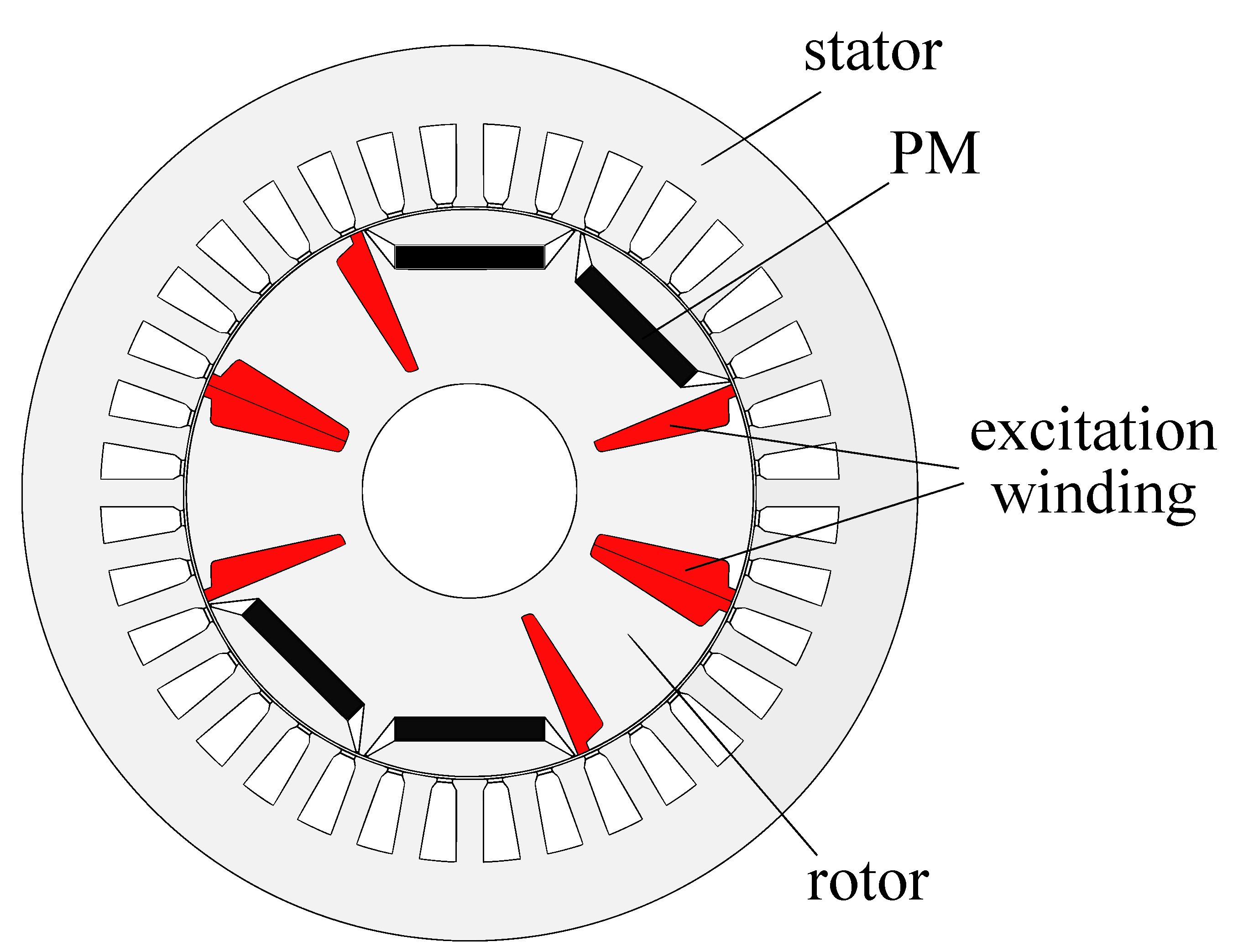
Here, a rotor typology is designed; its initial model is shown in Figure 1. Since the HEPM motor is characterized by a rotor with interior PMs, it is identified herein as an HE-IPM motor. Section 4 presents the finite element analysis of the HE-IPM designed in this work, highlighting the most relevant simulation results. The finite element analysis is performed to clarify the basic pole-changing motor operation and to verify the feasibility of the machine designed. Section 5 includes a parametric analysis of the rotor geometry, and Section 6 explains the performance of the dual-polarity HE-IPM (torque and power versus speed), comparing it to a traditional IPM motor. Finally, Section 7 presents a simple two-dimensional thermal analysis, and conclusions are drawn in the last section.

2. Double-Polarity Stator Winding

There are many winding configurations that allow for dual-polarity operation, as reported in [23]. Commonly, a change in polarity is realized by a switch that modifies the winding connections. In contrast, in this paper, the change in polarity is achieved by means of two inverters. As represented in Figure 2, in phase A, each phase of the stator winding is split into two parts. Half of the stator winding phase is supplied by inverter 1, and the other half by inverter 2.

The operating principle of this particular technique is described by means of the example in Figure 3, where four-coil winding is shown. This simple winding is supplied by two inverters, as described previously. In the top part of the figure, the two inverters supply the same current, giving rise to the magneto motive force (MMF) waveform reported below, which corresponds to a four-pole configuration. In the second part of the figure, the second inverter supplies an opposite current. The resulting MMF is modified and corresponds to a two-pole configuration.

The actual winding designed herein is a 36-slot double-layer winding. Its polarity can change from eight to four poles. Considering the eight-pole configuration, the slot angle is:

$${\alpha }_s^e=p·\frac{{360}^{\circ }}{Q_s}={40}^{\circ }$$

The number of slots per pole per phase is:

$$q_s=\frac{Q_s}{2p·m}=1.5$$

This means that it is a fractionary winding. The winding throw is $y_q=\frac{Q_s}{2p}=4.5$. The value of $y_q=4$, resulting in a chording angle of ${\beta }_r^e=0.5·{\alpha }_s^e={20}^{\circ }$. This particular angle allows a reduction in the seventh harmonic MMF. The resulting winding coefficient $k_w$ is calculated from the product of the pitch factor $k_p$ and the distribution factor $k_d$:

$$\begin{array}{cc}\hfill k_p& =cos\left(\frac{{\beta }_r^e}{2}\right)=0.985\hfill \\ \hfill k_d& =\frac{sin(q·\frac{{\alpha }_s^e}{2})}{q·sin\left(\frac{{\alpha }_s^e}{2}\right)}=0.975\hfill \\ \hfill k_w& =k_p·k_d=0.96\hfill \end{array}$$

When the current of the second inverter is reversed, the winding shifts to the four-pole configuration. The slot angle becomes:

$${\alpha }_s^e=p·\frac{{360}^{\circ }}{Q_s}={20}^{\circ }$$

And the number of slots per pole per phase is as follows:

$$q_s=\frac{Q_s}{2p·m}=3$$

The winding throw would be $y_q=9$, but the connections cannot be modified. Consequently, the chording angle is ${\beta }_r^e=5·{\alpha }_s^e={100}^{\circ }$. The resulting winding coefficient becomes much lower with this configuration:

$$\begin{array}{cc}\hfill k_p& =cos\left(\frac{{\beta }_r^e}{2}\right)=0.643\hfill \\ \hfill k_d& =\frac{sin(q·\frac{{\alpha }_s^e}{2})}{q·sin\left(\frac{{\alpha }_s^e}{2}\right)}=0.96\hfill \\ \hfill k_w& =k_p·k_d=0.62\hfill \end{array}$$

Consequently, since the winding is designed as an eight-pole configuration, the winding factor is higher when a high number of poles is achieved.

The winding connections are described hereafter.

Referring to phase $A^{\prime }$ (connected to the first inverter) and phase $A^{″}$ (connected to the second inverter), the coil side distribution within slots is represented by a slot matrix. Such a matrix contains as many elements as the number of slots. Each element represents the location of the phase coil side within each slot: the value is 1 if the coil side fills the whole slot (i.e., two layers), 0.5 if it occupies only half a slot (i.e., only one layer), and 0 if there is no coil side for that phase in the slot. The sign represents the reference current direction. The phase $A^{\prime }$ and phase $A^{″}$ slot matrices are as follows:

$$\begin{array}{cc}\hfill k_{A^{\prime }}=[& 0.5000-1-0.5000.50.500000000...\hfill \\ & 0.5000-1-0.5000.50.500000000]\hfill \\ \hfill k_{A^{″}}=[& 0.5000000000.5000-1-0.5000.5...\hfill \\ & 0.5000000000.5000-1-0.5000.5]\hfill \end{array}$$

For phases $B^{\prime }$, $B^{″}$, $C^{\prime }$, and $C^{″}$, the slot matrices must display ${120}^{\circ }$ electrical degrees; this corresponds to three slots (three elements of the vector). However, it is necessary to shift the ${120}^{\circ }$ of phase B by ${360}^{\circ }$ ($3+9=12$ slots) with respect to phase A. In fact, only by adding this shift can a correct arrangement of the windings be achieved when the polarity is changed to four. Figure 4 shows the eight-pole winding connections chosen herein.

When the current is reversed to change the pole number, both phase B and phase C are still connected to the same inverter (1 or 2), i.e., phases $B^{\prime }$ and $C^{\prime }$ are still connected to the first inverter, and phases $B^{″}$ and $C^{″}$ are still connected to the second inverter. This is due to the design choice of adding 360 electrical degrees in order to shift phase B with respect to phase A. Figure 5 shows the four-pole configuration. It is worth noting that phases $B^{\prime }$ and $C^{\prime }$ and phases $B^{″}$ and $C^{″}$ switch with each other; however, they are still connected to the same inverter as in the eight-pole configuration.

The total slot matrix for the winding, considering both inverter phase connections, is:

$$k=\left[\begin{array}{c}{k}_{A^{\prime }}+k_{A^{″}}\\ k_{B^{\prime }}+k_{B^{″}}\\ k_{C^{\prime }}+k_{C^{″}}\end{array}\right]=\left[\begin{array}{c}{k}_A\\ k_B\\ k_C\end{array}\right]$$

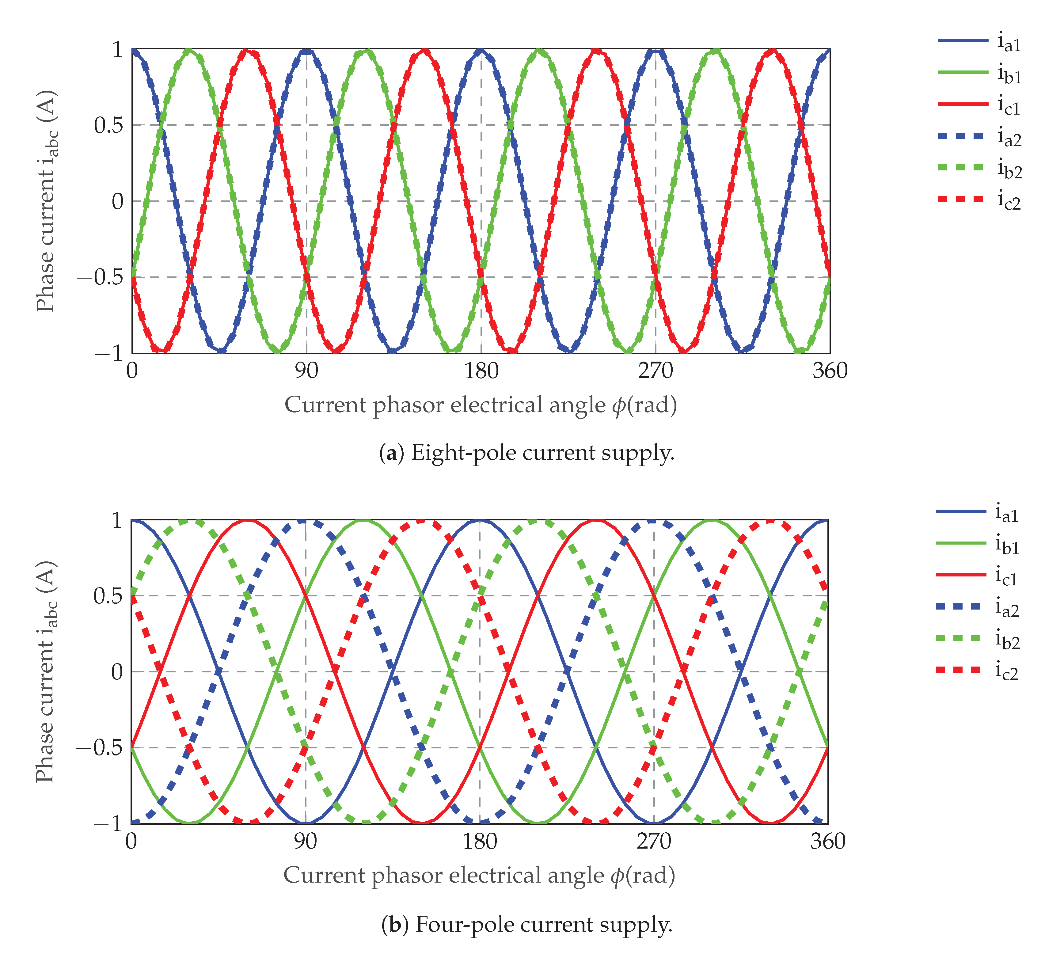
The MMF is analyzed considering the current supplied in Figure 6. The eight-pole current has half the four-pole current period. To obtain the eight-pole configuration, the first and second inverters have to supply the motor with two equal direct-sequence three-phase currents. The four-pole configuration is achieved when the second inverter current is reversed. In addition, the two inverters have to supply the motor with inverse-sequence three-phase currents. The four-pole configuration requires the inverse sequence of the three-phase current supply since, as observed in Figure 4 and Figure 5, phases $B^{\prime }$ and $C^{\prime }$ (and $B^{″}$ and $C^{″}$) switch with each other. Thus, the supply condition for dual-polarity operation can be summarized as:

$$\mathrm{Eight}-\mathrm{pole}\mathrm{configuration}:\left\{\begin{array}{c}{i}_{A^{\prime }}{i}_{B^{\prime }}{i}_{C^{\prime }}\hfill \\ i_{A^{″}}{i}_{B^{″}}{i}_{C^{″}}\hfill \end{array}\right.\mathrm{Four}-\mathrm{pole}\mathrm{configuration}:\left\{\begin{array}{c}{i}_{A^{\prime }}{i}_{C^{\prime }}{i}_{B^{\prime }}\hfill \\ -i_{A^{″}}-i_{C^{″}}-i_{B^{″}}\hfill \end{array}\right.$$

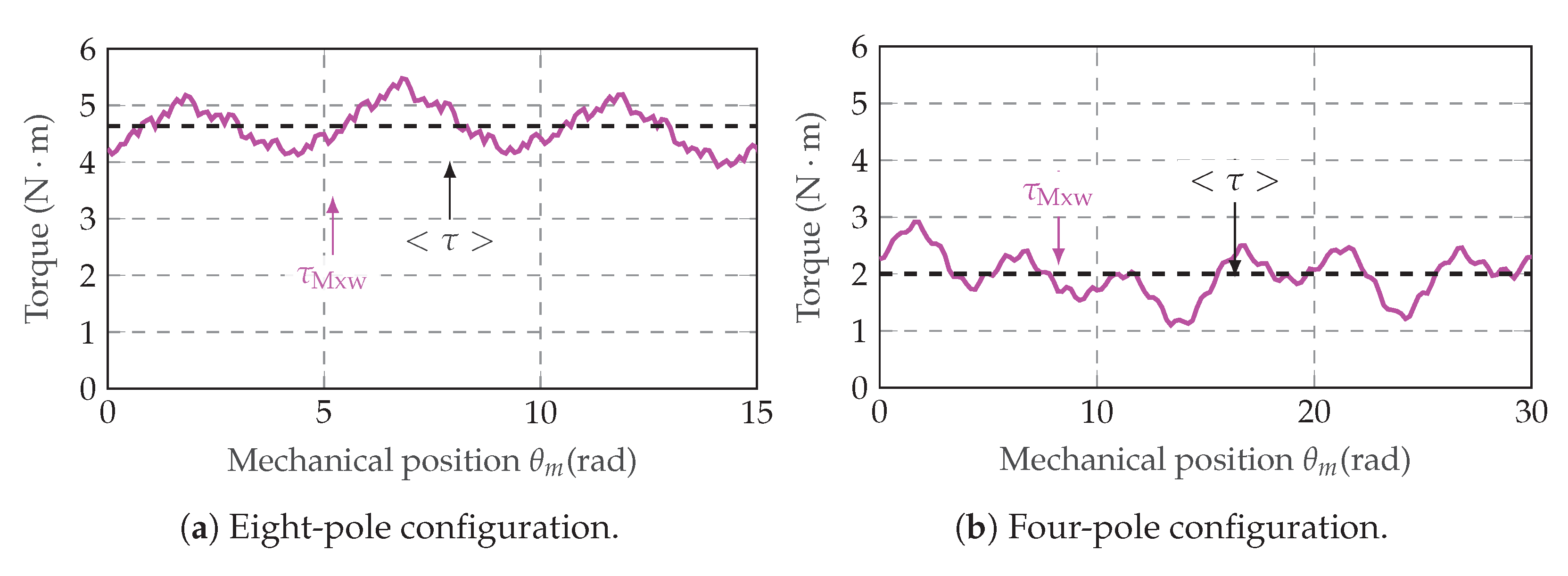
Figure 7 shows the MMF waveforms of the double-polarity winding, together with their harmonic content (from Fourier series expansion). The MMF is drawn for a rotor position that varies from 0 to 360 mechanical degrees, while the current phasor electrical angle is 0. It is worth noting that the eight-pole waveform is not symmetrical with respect to the x-axis, as expected for fractional slot winding. Concerning the Fourier analysis, both configurations exhibit good harmonic content thanks to the chorded double-layer winding design; this is the case even though the four-pole configuration presents a higher number of harmonics. This influences the torque ripple of this configuration.

Table 1. Stator data.

Parameter	Symbol	Value	Unit
External diameter	$D_e$	150	$\mathrm{m}\mathrm{m}$
Internal diameter	$D_s$	96	$\mathrm{m}\mathrm{m}$
Slot number	$Q_s$	36	-
Tooth width	$w_t$	13.14	$\mathrm{m}\mathrm{m}$
Slot cross-section area	$S_{slot}$	97.7	$\mathrm{m}{\mathrm{m}}^2$
Stack length	$L_{stk}$	40	$\mathrm{m}\mathrm{m}$
Iron pack length	$L_{fe}$	38.8	$\mathrm{m}\mathrm{m}$
Air gap width	g	0.5	$\mathrm{m}\mathrm{m}$
Poles	$2p$	8/4	-
Number of conductors per slot	$n_c=n_{cs}$	100	-
Conductor diameter	$d_c$	0.56	$\mathrm{m}\mathrm{m}$
Fill factor	$k_{fill}$	0.35	-
Nominal current	$I_N$	1.11	$\mathrm{A}$
Current density	$J_s$	5	$\mathrm{A}/\mathrm{m}{\mathrm{m}}^2$

summarizes stator geometric data and stator winding data.

3. Double-Polarity Rotor

3.1. Operating Principle

As the stator’s number of poles is changed, the rotor needs to adapt to the selected number of poles. This is carried out by means of parallel hybrid excitation thanks to the possibility of regulating the rotor coil current. Since PMs generate a constant magnetization flux, the excitation coils are supplied with a direct current. The rotor change in polarity is achieved by reversing that current.

Figure 8 shows the change in polarity principle. A rotor with only excitation coils is compared to the hybrid configuration considered in this study. The excitation-only rotor is able to switch from an eight-pole to a four-pole configuration by reversing the current of two consecutive coils. It is necessary to reverse the current of half the coils, as observed in the figure. Consequently, the supply condition of the other four coils does not change.

Since some coils are supplied by the same constant direct current in both an eight-pole and a four-pole configuration, they can be substituted with PMs, i.e., the constant magnetizing flux is the same. In this way, rotor losses decrease and, at the same time, the amount of rare earth material used is limited.

It is worth noting that, when a four-pole configuration is achieved, both PMs and excitation coils contribute to generating the rotor flux.

3.2. Design Considerations

As mentioned before, a rotor change in polarity is obtained with the HEPM motor configuration in Figure 1. Since this is a theoretical study, the initial design employed simple geometry based on the magnetic equivalent circuit (MEC) of the motor. The magnetic equivalent circuit method is useful for simple designs with fast and intuitive parameters, but it cannot derive the distribution of the magnetic field. Only the finite element method can provide an accurate magnetic field distribution; however, it requires a higher computational time. In this study, the MEC method is employed to design the initial rotor structure and, in particular, the PM dimensions.

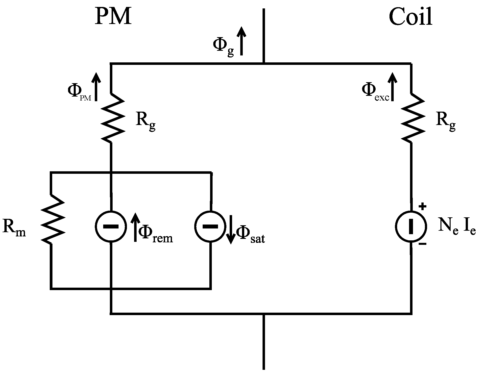
The PM pole no-load MEC is represented in Figure 9. Considering the desired no-load air-gap flux and the magnetic material properties of $NdFeBUH35$, the PM dimensions can be computed from the MEC equation. The parameters of the magnetic circuit are computed as follows:

$${\mathcal{R}}_g=\frac{g}{{\mu }_0·S_g}=\frac{g}{{\mu }_0·\frac{\pi D_s}{2p}·L_{stk}}$$

(1)

$${\mathcal{R}}_m=\frac{t_m}{{\mu }_{rec}·{\mu }_0·S_m}=\frac{t_m}{{\mu }_{rec}·{\mu }_0·l_m·L_{stk}}$$

(2)

$${\mathrm{\Phi }}_{rem}=B_{rem}·S_m=B_{rem}·l_m·L_{stk}$$

(3)

$${\mathrm{\Phi }}_{sat}=2·B_{sat}·t_{rib}·L_{fe}$$

(4)

$${\mathrm{\Phi }}_g=B_g·S_g=B_g·\frac{\pi D_s}{2p}·L_{stk}$$

(5)

The air gap is represented by the reluctance ${\mathcal{R}}_g$. The PM is represented by the parallel between the remaining reluctance associated with the material ${\mathcal{R}}_m$, the remaining flux ${\mathrm{\Phi }}_{rem}$, and the saturation flux ${\mathrm{\Phi }}_{sat}$ associated with the PM ribs. The value of the air-gap flux ${\mathrm{\Phi }}_g$ is set considering a flux density at the air gap equal to $B_g=0.8\mathrm{T}$.

g is the air gap, $S_g$ is the air gap surface, $t_m$ is the PM thickness, $S_m$ is its flux surface, $B_{rem}$ is the remaining flux of the PM employed, $B_{sat}$ is the saturation flux, $t_{rib}$ is the rib thickness, and $L_{fe}$ is the iron pack length.

Since all geometric parameters and material properties are known, the only unknown variables are the PM dimensions (radial length $l_m$ and thickness $t_m$). Considering a fixed ratio $l_m/t_m=6$, the MEC equation is solved as follows:

$$({\mathcal{R}}_g+{\mathcal{R}}_m)·{\mathrm{\Phi }}_g-{\mathcal{R}}_m·({\mathrm{\Phi }}_{rem}-{\mathrm{\Phi }}_{sat})=0$$

$$\Rightarrow {\mathrm{\Phi }}_{rem}=\frac{{\mathcal{R}}_g}{{\mathcal{R}}_m}·{\mathrm{\Phi }}_g+{\mathrm{\Phi }}_g+{\mathrm{\Phi }}_{sat}$$

(6)

Then, $l_m$ is computed from the resulting ${\mathrm{\Phi }}_{rem}$, and the result is equal to $26\mathrm{m}\mathrm{m}$. Values of $l_m=25\mathrm{m}\mathrm{m}$ and $t_m=4\mathrm{m}\mathrm{m}$ are chosen. Thus, by the solution of the magnetic equivalent circuit of the PM pole, the PM geometry is defined.

Considering the excitation coils, their design is strictly constrained by the limited space in the rotor. In fact, rotor slot shape is defined with an iterative method in order to limit iron saturation, both along the rotor tooth and close to the rotor shaft. In addition, the rotor slot area has to be large enough to limit the current density of the rotor. The resulting current density is equal to 10 $\mathrm{A}/\mathrm{m}{\mathrm{m}}^2$, which requires a water cooling system. In fact, heat removal is more challenging for the rotor than for the stator. Thermal aspects are considered in Section 7.

3.3. Excitation Current

The hybrid-excited motor designed herein is characterized by a rotor magnetization flux generated by both the PMs and the excitation coils. Since PMs produce a constant magnetization flux, the excitation current supplied has to be constant, and its magnitude has to be modulated in order to generate the same amount of flux as the PMs.

When a positive excitation current is supplied, the generated flux induces an alternate flux density distribution in the air gap, resulting in an eight-pole configuration. Then, when the excitation current is negative, the flux produced is reversed, so that it assumes the same direction of the flux produced by the PM of the adjacent pole. The resulting flux density distribution in the air gap corresponds to a four-pole configuration. Figure 10 shows how both configurations are achieved for the HE-IPM motor under study.

Both PMs and excitation coils are sources of the no-load rotor flux:

$${\mathrm{\Phi }}_g={\mathrm{\Phi }}_{PM}+{\mathrm{\Phi }}_{exc}$$

Thus, the excitation current is non-zero during the no-load operation. Therefore, the excitation current is chosen according to the no-load analysis of the motor. In particular, the air-gap flux density due to the PMs has to be equal to the air-gap flux density due to the excitation coils. An initial value is computed considering the magnetic equivalent circuit of both the PMs and the excitation coils, as seen in Figure 11. The two MECs are characterized by the same air-gap flux ${\mathrm{\Phi }}_g$. The parameters of the magnetic circuit are computed as already described in Equations (1)–(4). To achieve a constant air-gap flux ${\mathrm{\Phi }}_g$, ampere-turns $N_e{I}_e$ yield a result of 500 A-turns. Then, this value is adjusted to attain a proper air-gap flux density waveform. In addition, the value is chosen to reduce the harmonic content of the four-pole no-load flux linkage. This is performed by adjusting the excitation current and evaluating the flux linkage. Thus, the excitation ampere-turns are as follows:

$$N_e{I}_e=450\mathrm{A}-\mathrm{turns}$$

Table 2. Rotor data.

Parameter	Symbol	Value	Unit
Rotor diameter	$D_r$	95	$\mathrm{m}\mathrm{m}$
PM thickness	$t_m$	4	$\mathrm{m}\mathrm{m}$
PM length	$l_m$	25	$\mathrm{m}\mathrm{m}$
Distance PM air gap	$d_{gm}$	10	$\mathrm{m}\mathrm{m}$
Excitation length	$h_{exc}$	25	$\mathrm{m}\mathrm{m}$
Excitation upper width	$w_{exc,u}$	6	$\mathrm{m}\mathrm{m}$
Excitation lower width	$w_{exc,l}$	2	$\mathrm{m}\mathrm{m}$
Number of conductors per slot	$N_e$	220	-
Nominal current	$I_e$	2.05	$\mathrm{A}$
Conductor diameter	$d_{c,r}$	0.5	$\mathrm{m}\mathrm{m}$
Fill factor	$k_{fill,r}$	0.44	-
Current density	$J_e$	10	$\mathrm{A}/\mathrm{m}{\mathrm{m}}^2$

summarizes the rotor geometric data and rotor winding data. Both the stator and rotor laminations are of $M53050A$ type, and the PMs are $NdFeBUH35$.

Figure 12 shows the flux lines and the flux density map for the HE-IPM motor in the no-load condition. The flux line distributions are different for the four-pole configuration and the eight-pole configuration, as expected due to the difference in pole numbers. The back-iron flux density is much higher when the four-pole configuration is employed. Thus, to reduce saturation and iron power losses, the back-iron thickness has to be designed according to the low polarity flux.

Figure 13 shows the no-load flux density waveform along the air gap achieved with four-pole and eight-pole excitation.

4. Finite Element Analysis

Two-dimensional magneto static finite element simulations are carried out to verify the dual-polarity operation of the motor designed as described in Section 3. The finite element analysis software employed is FEMM 4.2. FEMM is a suite of programs for solving low-frequency electromagnetic problems in two-dimensional domains. The pre- and post-processing programs employed were written by the University of Padova research team.

4.1. No-Load Analysis

The first step is the no-load finite element analysis of the HE-IPM motor. After the alignment of the IPM rotor, no-load flux linkages are computed as:

$${\lambda }_j=n_{cs}·L_{fe}·\sum _{q=1}^Q{k}_{j,q}·\frac{1}{S_{slot}}{\int }_{S_{slot}}{A}_{z}dS\mathrm{j}=\mathrm{A},\mathrm{B},\mathrm{C}$$

(7)

where $k_{j,q}$ is the slot matrix value of phase j for the slot q, and $A_z$ is the magnetic scalar potential. Since the two-inverter slot matrices are defined separately, the fluxes linked by the first and second inverter are computed separately as well:

$${\lambda }_{j^{\prime }}=n_{cs}·L_{fe}·\sum _{q=1}^Q{k}_{j^{\prime },q}·\frac{1}{S_{slot}}{\int }_{S_{slot}}{A}_{z}dS$$

(8)

$${\lambda }_{j^{″}}=n_{cs}·L_{fe}·\sum _{q=1}^Q{k}_{j^{″},q}·\frac{1}{S_{slot}}{\int }_{S_{slot}}{A}_{z}dS$$

(9)

Figure 14 shows the no-load flux linkages. The flux linkages of the first and second windings almost overlap during eight-pole operation. On the contrary, they are opposite in the four-pole configuration. As expected, the eight-pole configuration period is exactly half that of the four-pole configuration period. In addition, the four-pole configuration is characterized by more distorted waveforms. The greater distortion of the four-pole flux linkage waveform compared to the eight-pole one is related to the nature of the four-pole configuration itself. In fact, the four-pole configuration is obtained from the eight-pole geometry, with a reversed excitation current. The current inversion affects the four-pole air-gap flux density waveform and, consequently, the flux linkage waveform. When the number of poles changes from eight to four, the fundamental harmonic winding factor $k_{w,1}$ is reduced, but the higher harmonic winding factor $k_{w,\nu }$ increases.

4.2. On-Load Analysis

The on-load finite element analysis is carried out considering the specific rotor alignment for each of the two polarities. Indeed, the d-axis and the q-axis have different relative positions depending on the number of poles of the machine. Both motors operate with the maximum torque per ampere (MTPA), which also differs between the eight-pole and four-pole configurations. The four-pole torque is lower than the eight-pole torque. As such, the current phasor electrical angle for MTPA operation is slightly different due to the different saliency factor (i.e., a different ratio between the q-axis and d-axis inductances).

Considering the MTPA supply condition, the torque is computed for different rotor mechanical positions to obtain the average torque in a period, as well as the oscillations. Figure 15 shows the torque for one period. The torque computed by means of Maxwell’s stress tensor is indicated as ${\tau }_{Mxw}$, while its average value is indicated by <$\tau$>. The eight-pole torque waveform period is 15 mechanical degrees, while the four-pole torque waveform period is exactly twice the period of the configuration with a higher pole number (i.e., 30 mechanical degrees), as expected. The four-pole configuration is characterized by half the average torque of the eight-pole configuration, along with a higher torque ripple, as expected from the higher harmonic content highlighted above. Indeed, the four-pole flux density and flux linkage waveforms are not perfectly sinusoidal, which is the case for those of the eight-pole.

The resulting mean torque is equal to 4.6 $\mathrm{N}·\mathrm{m}$ for the eight-pole configuration and 1.9 $\mathrm{N}·\mathrm{m}$ for the four-pole configuration. The torque ripple is 34% for the eight-pole machine and 90% for the four-pole machine.

5. Parametric Analysis

As examined previously, the resulting torque ripple is too high, in particular when the four-pole configuration is employed. To achieve a smooth torque waveform, several design solutions can be taken into consideration:

• Skewing of the stator pack;
• Skewing of the rotor pack;
• Rotor pole shaping.

Concerning the first solution, the skewing of the stator pack is barely used due to winding manufacturing difficulties. In contrast, the use of rotor skewing is more common, despite the fact that it is more complex, with a hybrid-excitation rotor. Indeed, the presence of excitation coils requires continuous skewing, which is very expensive for PMs. Herein, it was decided to employ step-skewing of the PMs [24], inserting them into a continuously skewed hole, as depicted in Figure 16. Since the skewing angle is equal to 10${}^{\circ }$, a step-skewing equal to 5 is chosen. Thus, a single PM is divided into five parts, which represent the five steps of the discrete skewing. In this way, the PM width $w_{PM,skew}$ has an additional constraint, since it has to be smaller than the PM housing width $w_{PM}$.

To compute the step-skewing 2D simulation, five different simulations are carried out, one for each section of the skewed geometry. In other words, each of the five simulations is carried out with a different rotor shift (-4${}^{\circ }$, -2${}^{\circ }$, 0${}^{\circ }$, 2${}^{\circ }$, and 4${}^{\circ }$). More precisely, the same motor model magneto static simulation is carried out five times with the additional constant rotor angle ${\theta }_{m,skew}$. Thus, the rotor position of each j${}^{th}-$simulation varies with the law:

$${\theta }_m^j={\theta }_{m,skew}^j+{\theta }_m\mathrm{with}j=1,2,3,4,5$$

where ${\theta }_{m,skew}^j$ is equal to the additional skewing angle, which corresponds to the mean position of the section considered with respect to the central PM that serves as the reference (with ${\theta }_{m,skew}^0=0^{\circ }$). Figure 17 shows such a simulation setup.

The skewing simulation gives the result for a step-skewed machine, even if, for rotor excitation, the skewing is continuous.

Thus, considering the HE-IPM with the skewing solution described, the resulting torque ripple is reduced, as shown in Figure 18. The results of the skewing solution are a mean torque of 4.4 $\mathrm{N}·\mathrm{m}$ for the eight-pole configuration and 2 $\mathrm{N}·\mathrm{m}$ for the four-pole configuration. The configuration with the higher number of poles decreases from a 34 % torque ripple to 3.5 %, while the configuration with the lower number of poles is reduced from 90 % to 22 %.

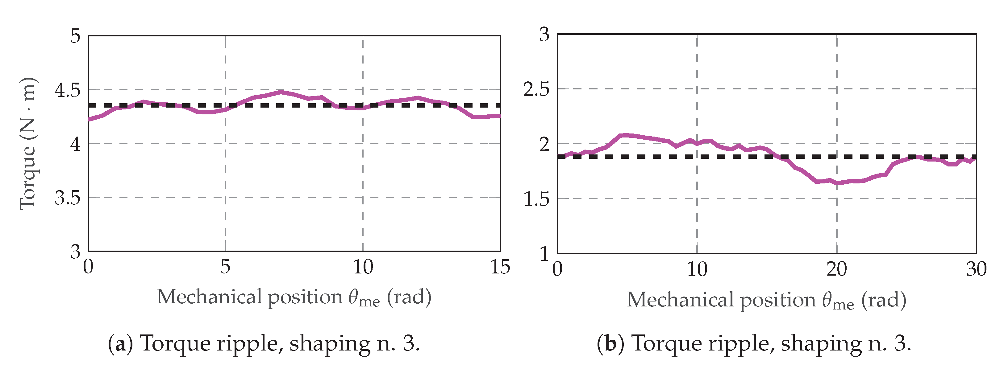
The third solution consists in modifying the HE-IPM motor to properly shape the rotor. Figure 19 shows two parameters that can be modified to properly shape the rotor: the maximum distance to the stator $d_{s,max}$ and the arc angle ${\alpha }_s$. As an example, four different rotor configurations, with the shaping parameters described in

Table 3. Torque ripple with the shaped rotor solution.

HE-IPM	Parameter	8 Poles	4 Poles
non-shaped
$d_{s,max}=47.5^{\circ }$	Average torque <$\tau$>	4.6 $\mathrm{N}·\mathrm{m}$	1.9 $\mathrm{N}·\mathrm{m}$
${\alpha }_s=0.5\mathrm{m}\mathrm{m}$	Percentage ripple	34%	90%
shaping n.1
$d_{s,max}={47}^{\circ }$	Average torque <$\tau$>	4.21 $\mathrm{N}·\mathrm{m}$	1.9 $\mathrm{N}\mathrm{m}$
${\alpha }_s=1\mathrm{m}\mathrm{m}$	Percentage ripple	14.9%	45.2%
shaping n.2
$d_{s,max}={30}^{\circ }$	Average torque <$\tau$>	4.65 $\mathrm{N}\mathrm{m}$	2 $\mathrm{N}\mathrm{m}$
${\alpha }_s=1\mathrm{m}\mathrm{m}$	Percentage ripple	9.2%	36%
shaping n.3
$d_{s,max}={35}^{\circ }$	Average torque <$\tau$>	4.7 $\mathrm{N}\mathrm{m}$	2 $\mathrm{N}\mathrm{m}$
${\alpha }_s=1.5\mathrm{m}\mathrm{m}$	Percentage ripple	5.9%	30.8%
shaping n.4
$d_{s,max}={30}^{\circ }$	Average torque <$\tau$>	4.35 $\mathrm{N}\mathrm{m}$	1.88 $\mathrm{N}\mathrm{m}$
${\alpha }_s=1.5\mathrm{m}\mathrm{m}$	Percentage ripple	5.9%	23%

, are analyzed. It is worth noting that the torque waveform becomes smoother as the rotor shaping increases. Nevertheless, as the shaping increases, the air gap volume increases as well; thus, the torque mean value is slightly decreased. Nevertheless, the eight-pole configuration performance results are always better than those of the four-pole configuration due to the fact that both flux linkage and torque waveform worsen when the excitation current is reversed. The best configurations for eight-pole and four-pole torque ripple (n. 4) are presented in Figure 20.

6. Mechanical Characteristics

6.1. Torque and Power versus Speed of the HE-IPM Motor

Another finite element analysis is conducted to examine a possible electric drive for this machine. Torque and power versus speed characteristics can be obtained through magneto static simulations under different loading conditions. The eight-pole and four-pole HEPMs are considered separately, and they are fed with a constant current amplitude and a variable current phasor angle. The rotor excitation current is maintained at a constant, and it is reversed only when the four-pole configuration is analyzed.

The speed reached for each operating point is computed from the d-axis and q-axis flux linkage values, considering a constant DC bus voltage $V_{DC}$ with PWM control and a certain drop in voltage ($\Delta V$):

$${\omega }_B=\frac{1/\sqrt{3}·V_{DC}-\Delta V}{\sqrt{{\lambda }_D^2+{\lambda }_Q^2}}$$

(10)

where ${\lambda }_D$ and ${\lambda }_Q$ are the flux linkages computed from the ABC values to the d- and q-axis values, respectively.

The MTPA current is supplied until the base speed is reached, resulting in a constant torque region. Then, the current angle is increased, reducing the torque value until it reaches zero, when the maximum speed is achieved. The power increases linearly until the base speed is achieved; then, it reaches its maximum at a higher speed and becomes zero at the maximum speed.

Both the torque and power mechanical characteristics of the HE-IPM motor under analysis are reported in Figure 21. When the eight-pole configuration is employed, the motor exhibits high torque at low speeds, while the four-pole configuration is characterized by a lower level of torque but a wider speed range. Thus, the eight-pole configuration is suitable for start-up, as it has a high starting torque. However, its speed range is limited. It is possible to switch to the four-pole configuration in order to extend the range of speeds. The main performance parameters are summarized in

Table 4. Mechanical characteristics: data comparison.

Parameter	8 Poles	4 Poles
Base speed ${\omega }_B$	1010 $\mathrm{r}/\min$	2810 $\mathrm{r}/\min$
Maximum speed ${\omega }_M$	1330 $\mathrm{r}/\min$	3090 $\mathrm{r}/\min$
MTPA torque $\tau$	4.6 $\mathrm{N}\mathrm{m}$	1.9 $\mathrm{N}\mathrm{m}$

.

6.2. Comparison between HE-IPM and a Traditional IPM Motor

In order to underline the advantage of this machine, the dual-polarity HEPM motor is compared to a traditional IPM motor. Two different magnetizing flux IPM motors are considered and compared to the non-shaped and non-skewed HE-IPM motor. The first IPM’s geometry is designed in the same way as the HE-IPM analyzed but without excitation coils. All poles are made of $NdFeB$ PMs of the same type and dimensions as the HEPM PMs, as represented in Figure 22a.

The other IPM is designed with a lower PM volume, as represented in Figure 22b. A lower volume of magnetic material leads to a lower magnetizing flux and, thus, a lower torque with respect to the requirements of the eight-pole motor. However, the reduction in the magnetizing flux allows having an extended FW region, i.e., a higher maximum speed. Consequently, the resulting motor has an intermediate performance between high torque and high speed.

The comparison between the HE-IPM and the two traditional IPM motors is shown in Figure 23. The machine in Figure 22a exhibits the same performance as the eight-pole HE-IPM since it is designed by substituting rotor excitation coils with identical PMs. The machine in Figure 22b is characterized by an extended flux-weakening operation; thus, it has a higher maximum speed, but its torque is lower. This is related to the lower PM volume of the machine. In fact, the reduction in the magnetization flux leads to a lower torque. At the same time, the lower flux linkage allows reaching higher speeds when supplying the same DC bus voltage.

Table 5. Rated speed performance comparison between HE-IPM and IPM.

Parameter	8-Pole HE-IPM	4-Pole HE-IPM	IPM Case 1	IPM Case 2
Rated speed ${\omega }_B$	1010 $\mathrm{r}/\min$	2810 $\mathrm{r}/\min$	1000 $\mathrm{r}/\min$	2810 $\mathrm{r}/\min$
MTPA torque $\tau$	4.4 $\mathrm{N}\mathrm{m}$	1.9 $\mathrm{N}\mathrm{m}$	4.3 $\mathrm{N}\mathrm{m}$	0 $\mathrm{N}\mathrm{m}$
Efficiency $\eta$	76 %	67 %	89 %	0
Joule losses $P_J$	141.5 $\mathrm{W}$	260 $\mathrm{W}$	520 $\mathrm{W}$	0 $\mathrm{W}$
Iron losses $P_{fe}$	8 $\mathrm{W}$	24 $\mathrm{W}$	3.5 $\mathrm{W}$	0 $\mathrm{W}$
Output power $P_{out}$	470 $\mathrm{W}$	560 $\mathrm{W}$	460 $\mathrm{W}$	0 $\mathrm{W}$
Power factor $PF$	0.97	0.99	0.93	0

shows the performance comparison between the HE-IPM motor and the first IPM motor when the rated speed is reached. Motor losses are computed as described in Appendix A and Appendix B, then the efficiency is obtained as in Appendix C. The HE-IPM motor has a lower efficiency at the rated speed due to the additional joule losses of the rotor coils. Such rotor joule losses are high in this small-sized motor but have a very small influence on the total losses in high-power applications. In fact, large-sized motors that use rotor excitation current are characterized by high efficiency, despite the additional rotor losses.

As shown in Figure 24, the IPM motor efficiency drops for speeds higher than 1250 $\mathrm{r}/\min$, while the HE-IPM continues to operate with higher efficiency. In addition, for speeds higher than 1320 $\mathrm{r}/\min$, the IPM motor does not provide power, while the HE-IPM continues to operate.

In addition, the HE-IPM machine displays improved torque versus speed capabilities thanks to the possibility of changing the number of poles. In fact, by regulating the excitation current and without changing the rotor geometry, the speed range can be extended up to more than double the maximum speed of the eight-pole configuration. In contrast, the speed range of traditional IPM motors can be regulated only by changing PM dimensions, i.e., by modifying the motor geometry. The dual-polarity HEPM machine allows it to perform like two machines with only one hybrid-excited configuration.

In addition, it is possible to vary the HE-IPM field during flux-weakening operation to enhance performance. An example of this control strategy is presented in Figure 25. The rotor current is reduced, lowering the rotor flux. Thus, the torque slightly decreases while the speed range is gradually extended. Consequently, the motor efficiency increases, since rotor joule losses decrease as the excitation current is reduced.

7. Thermal Considerations

In the literature, several thermal studies on wound rotor machines have been conducted [25,26,27,28]. Salient pole synchronous machines provide high efficiency, low noise, and low vibration [29,30,31]. In addition, they should have excellent thermal stability, especially because windings are placed in the rotor as well. To consider the thermal stability of the machine under study, a thermal analysis is carried out in parallel to the electromagnetic study. In this work, a simple two-dimensional finite element thermal study is presented. For the thermal finite element analysis, the motor model is the same model used for the magneto static simulations.

Two different cooling systems are considered, and their performance is compared. The first is a water cooling system, with water flowing in tubes along the motor case. The second is based on a classical finned case, cooled by forced air, but with an additional cooling system in the motor shaft that consists in oil flowing along the shaft itself [32,33].

Simulations are carried out in order to determine the heat exchange parameters such that the temperature rise of the rotor winding remains lower than:

$$\Delta T_{winding,r}=125{}^{\circ }\mathrm{C}$$

Calculations are performed considering class H of insulation, with a maximum environmental temperature of 40 ${}^{\circ }\mathrm{C}$.

To solve the thermal finite element problem, boundary conditions have to be imposed to specify the convection heat transfer coefficient h and impose an environmental temperature $T_0$ equal to 0 $\mathrm{K}$. Thus, the simulation result represents the temperature increase for each motor region. Since half the machine is simulated, periodic boundary conditions are imposed along the lines that divide the motor in half.

In addition to the thermal study of the HE-IPM motor, other thermal simulations are presented in this section to compare the thermal performance of the IPM and HEPM machines.

7.1. Water Cooling System

The thermal finite element simulation model is represented in Figure 26. The external holed layer represents the motor aluminium case through which the cooling water flows. Between the motor and the case, there is a 0.02 $\mathrm{m}\mathrm{m}$ still air layer. To avoid a too-small mesh size, this layer is modelled as a 2 $\mathrm{m}\mathrm{m}$ layer with a thermal conductivity 100 times higher than that of still air (0.02 $\mathrm{W}/(\mathrm{m}·\mathrm{K})$), i.e., 2 $\mathrm{W}/(\mathrm{m}·\mathrm{K})$. All other regions, depending on the material and the possible fluid motion, have different thermal conductivities that are summarized in

Table 6. Parameters of the thermal finite element simulation.

Region	Thermal Conductivity $\mathit{\lambda }$	Heat Generation $\mathit{P}/\mathit{Vol}$
	W/(m $\mathit{·}$ K)	W/m${}^3$
Shaft steel	22	0
Stator iron stack	30	25,160
Rotor iron stack	30	0
Permanent magnet	10	0
Still air (ribs)	0.02	0
Still air (stator case)	2	0
Rotor copper winding	1	328,6482
Winding insulation	1	0
Air gap air	0.1	0
Stator copper winding	1	601,619
Aluminium case	200	0

.

It is worth noting that the air gap is characterized by a thermal conductivity five times higher than that of still air due to rotor motion. In fact, the air between the rotor external surface and the stator internal surface is not still, but the fluid layer that is in contact with the rotor is moving at the same speed as the rotor. Based on the study of the thermal flow in a salient pole motor, for a similar size motor at a rated speed of 1000 $\mathrm{r}/\min$, a feasible convection heat transfer coefficient h is 300 $\mathrm{W}/({\mathrm{m}}^2·\mathrm{K})$. Thus, considering the surface S through which the heat flow occurs, balancing the heat exchanged through conduction and the heat exchanged through convection along the air gap:

$$\frac{g}{\lambda ·S}=\frac{2}{h·S}$$

the thermal conductivity of the air gap $\lambda$ is computed:

$$\lambda =\frac{h·g}{2}\approx 0.1$$

In addition to the thermal problem settings, the heat generated by each region is also specified in Table 6. The heat generated by the motor is computed by a single magneto static simulation at the rated speed ${\omega }_B$. Both the rotor and stator windings produce heat due to joule losses; thus, their contributions to the temperature increase are considered separately as $P_{J,s}$ and $P_{J,r}$. In addition, stator iron losses $P_{fe}$ are taken into account for the thermal analysis. In the thermal problem, each region that generates heat flux is defined by specific power losses, i.e., the ratio between power losses and the volume of the region. All data are summarized in

Table 7. Power losses and specific losses of the eight-pole HE-IPM at the rated speed ${\omega }_B=1010\mathrm{r}/\min$.

Parameter	Value
Stator joule losses $P_{J,s}$	51.84 $\mathrm{W}$
Rotor joule losses $P_{J,r}$	89.61 $\mathrm{W}$
Total joule losses $P_J$	141.5 $\mathrm{W}$
Iron losses $P_{fe}$	8 $\mathrm{W}$
Stator winding copper volume $Vo{l}_s$	$2.39\times {10}^{-6}$${\mathrm{m}}^3$
Rotor winding copper volume $Vo{l}_r$	$3.41\times {10}^{-6}$${\mathrm{m}}^3$
Stator iron stack volume $Vo{l}_{fe,s}$	$3.18\times {10}^{-4}$${\mathrm{m}}^3$
Specific stator joule losses $P_{J,s}/(Vo{l}_s·Q_s)$	601,619 $\mathrm{W}/{\mathrm{m}}^3$
Specific rotor joule losses $P_{J,r}/(Vo{l}_r·Q_r)$	3,286,482 $\mathrm{W}/{\mathrm{m}}^3$
Specific iron losses $P_{fe}/Vo{l}_{fe}$	25,160 $\mathrm{W}/{\mathrm{m}}^3$

.

Finally, boundary conditions are imposed to solve the finite element problem. Periodic boundary conditions are imposed along the lines that divide the motor in half. On the external case surface, an air-free convection heat exchange is imposed, with coefficient:

$$h=5\mathrm{W}/({\mathrm{m}}^2·\mathrm{K})$$

Then, the thermal simulation is carried out to verify the fluid condition required to reach acceptable temperatures. Figure 27 shows the simulation result. The temperature increase is very low along the aluminium case and also in the stator, thanks to the water cooling system. Due to the high current density of the rotor excitation coils, the temperature increase in the rotor is higher than in the stator.

The rotor slots that face each other are characterized by the highest temperature increases, while the rotor slots close to the PMs reach lower temperatures. The highest temperature increase is equal to 112 $\mathrm{K}$, which is acceptable considering the class H of insulation. In addition, it is worth noting that the temperature of the PMs is acceptable as well. In fact, the magnetic material adopted, PM $NdFeBUH35$, can sustain a maximum temperature of 180 ${}^{\circ }\mathrm{C}$ due to demagnetization problems.

The resulting convective coefficient obtained from the simulations is equal to:

$$h=500\mathrm{W}/({\mathrm{m}}^2·\mathrm{K})$$

This corresponds to water flowing in tubes in a cooling system selected for such a high rotor current density motor. This coefficient is imposed as a boundary condition along all the lines that represent pipes filled with water. The other boundary condition imposed is the temperature, equal to $T_0=0\mathrm{K}$, as explained in the introduction to this section.

7.2. Air and In-Shaft Oil Cooling System

The alternative cooling system model considered is represented in Figure 28. The external aluminium case is completely finned in order to favour heat transfer. The 0.02 $\mathrm{m}\mathrm{m}$ layer is modelled as in the water cooling model described previously. The thermal conductivities of all regions are the same as in the water cooling model, as summarized in Table 6. In addition, the air gap thermal conductivity is the same since both simulations refer to the rated speed operation.

Along the finned surface of the case, the boundary condition of forced air convection is imposed:

$$h=20\mathrm{W}/({\mathrm{m}}^2·\mathrm{K})$$

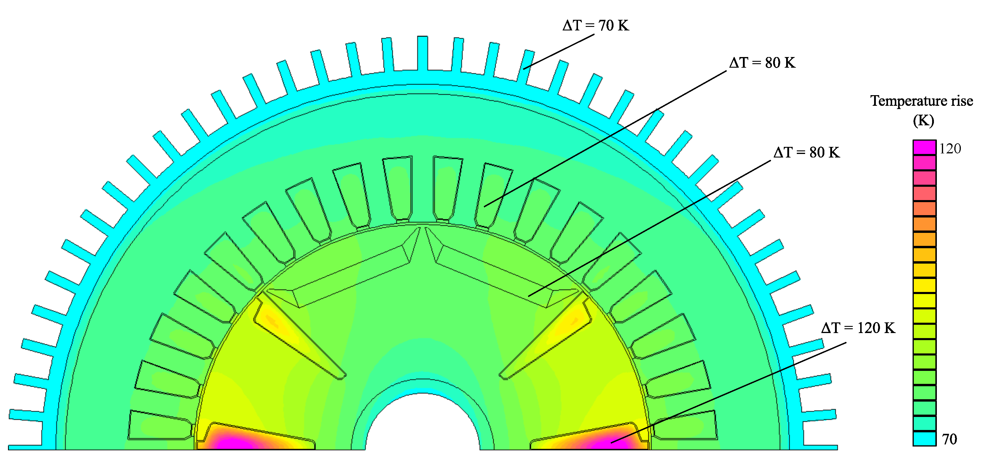
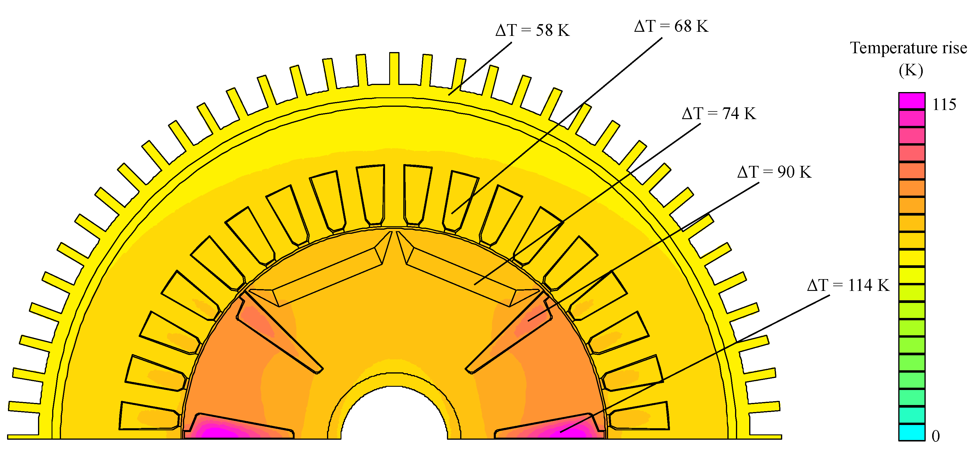
Then, the thermal simulation is carried out to verify the fluid condition required to reach acceptable temperatures. Figure 29 shows the simulation result. Similar to the water cooling system, the highest temperature increase in the rotor windings is equal to 114 $\mathrm{K}$, which is acceptable considering the class H of insulation. The rotor slots that face each other are characterized by the highest temperature increases, while the rotor slots close to the PMs reach lower temperatures. In addition, the temperature of the PMs is acceptable and is the same as in the water cooling model.

The main difference between this water-and-oil cooling system and the previously analyzed water cooling system is the gradient of the temperature increase. In fact, the external air does not have the same cooling effectiveness as water. In contrast, the rotor heat is effectively dissipated by the oil flowing inside the motor shaft. As a result, the temperature increase of the rotor is comparable between the two models, while the temperature increase reached on the external case for the water-and-oil model is equal to 58 $\mathrm{K}$; in the stator slots, it is 68 $\mathrm{K}$ (versus the water cooling results of 5 $\mathrm{K}$ and 24 $\mathrm{K}$, respectively).

The resulting convective coefficient obtained from the simulations is equal to:

$$h=350\mathrm{W}/({\mathrm{m}}^2·\mathrm{K})$$

This corresponds to oil flowing with free convection inside the motor shaft. Such a coefficient is imposed as a boundary condition along the internal shaft line.

7.3. Comparison with the IPM Motor: Air Cooling System

The traditional IPM motor studied in Section 6.2 is considered here for a comparison of thermal behaviour. A forced-air cooling system is adopted, as represented in the model in Figure 30. With respect to the rated point operation considered, the thermal conductivity values for all regions of the motor and the thermal losses are reported in Table 6. Along the external case surface, which is finned and cooled by forced air, a convective heat transfer boundary condition is imposed, with the following parameters:

$$h=15\mathrm{W}/({\mathrm{m}}^2·\mathrm{K})$$

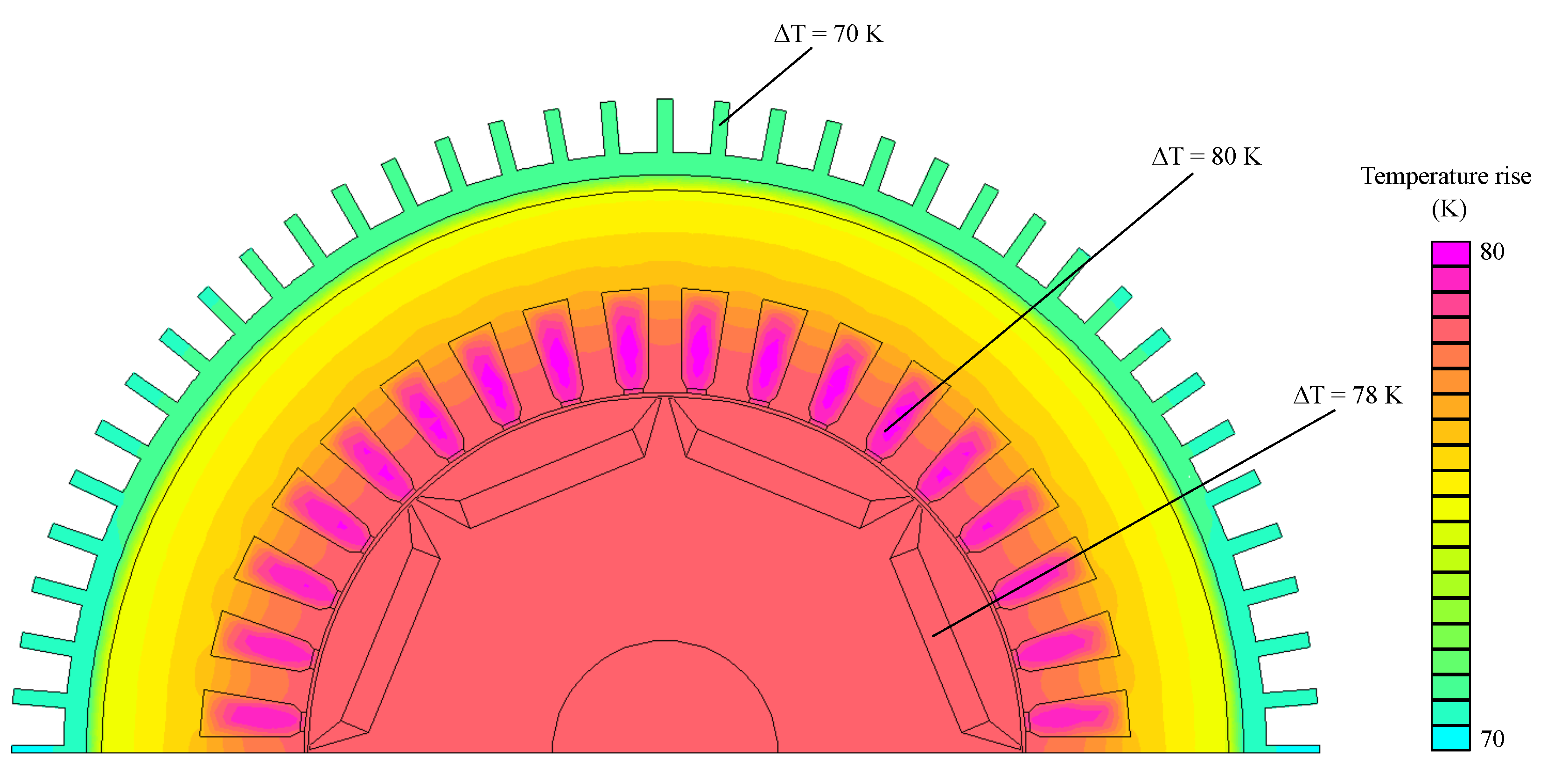
Figure 31 shows the thermal simulation result. The temperature increase varies from 70 $\mathrm{K}$ to 80 $\mathrm{K}$. The stator winding temperature increase is equal to 80 $\mathrm{K}$, similar to that of the PMs and the whole rotor core.

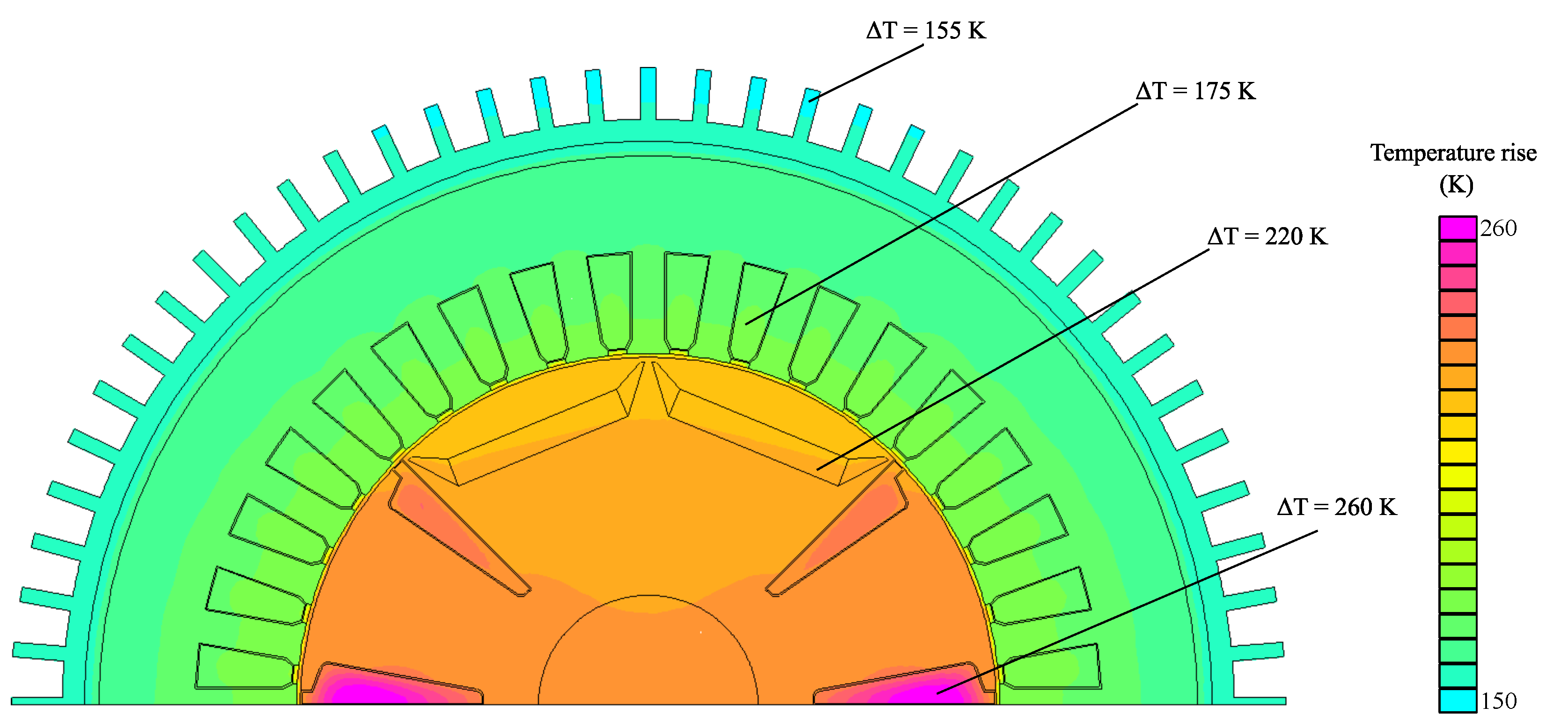
Figure 32 shows the thermal simulation result for the HEPM motor with the same air cooling system as the IPM motor. The temperature increase is too high, leading to the burning of windings insulation and the demagnetization of PMs. It is worth noting that the rotor temperatures are higher than those of the stator. This is due to the low air gap thermal conductivity, which limits heat transfer from the rotor to the stator. Hence, the air cooling system is effective for the stator but does not allow for good rotor heat dissipation.

This thermal simulation proves that the hybrid-excited motor cannot be cooled using the same strategy as an IPM motor. In fact, the rotor windings generate additional heat in the rotor core; this heat is hard to dissipate due to the air gap.

Considering the presence of additional rotor windings, the HEPM motor cooling system has to be improved. Thus, an additional rotor cooling system is adopted that forces oil flow inside the shaft. Figure 33 shows the HEPM motor temperature increases with this improved cooling system. To reach a maximum temperature increase of about 120 $\mathrm{K}$ in the rotor windings, the convective heat transfer coefficient imposed for the inner surface of the shaft is:

$$h=350\mathrm{W}/({\mathrm{m}}^2·\mathrm{K})$$

It is worth noting that the PM temperature increase is sufficiently low to avoid demagnetization (80 $\mathrm{K}$); in addition, the rotor windings are limited to an acceptable temperature increase (120 $\mathrm{K}$).

Table 8. Comparison of the thermal performance of the IPM and HEPM motors with the same stator losses.

	IPM Motor	HEPM Motor	HEPM Motor
Parameter	Stator Water Jacket	Stator Water Jacket	Stator Water Jacket +
			Shaft Oil Cooling
Stator winding $\Delta T$	80 ${}^{\circ }\mathrm{C}$	175 ${}^{\circ }\mathrm{C}$	80 ${}^{\circ }\mathrm{C}$
PMs $\Delta T$	78 ${}^{\circ }\mathrm{C}$	220 ${}^{\circ }\mathrm{C}$	80 ${}^{\circ }\mathrm{C}$
Rotor winding $\Delta T$	/	260 ${}^{\circ }\mathrm{C}$	120 ${}^{\circ }\mathrm{C}$
Rated speed ${\omega }_B$	1000 $\mathrm{r}/\min$	1010 $\mathrm{r}/\min$	1010 $\mathrm{r}/\min$
MTPA torque $\tau$	4.3 $\mathrm{N}\mathrm{m}$	4.4 $\mathrm{N}\mathrm{m}$	4.4 $\mathrm{N}\mathrm{m}$
Efficiency $\eta$	89 %	76 %	76 %
Joule losses $P_J$	520 $\mathrm{W}$	141.5 $\mathrm{W}$	141.5 $\mathrm{W}$
Iron losses $P_{fe}$	3.5 $\mathrm{W}$	8 $\mathrm{W}$	8 $\mathrm{W}$
Output power $P_{out}$	460 $\mathrm{W}$	470 $\mathrm{W}$	470 $\mathrm{W}$
Power factor $PF$	0.93	0.97	0.97

compares the thermal performance of the IPM and HEPM motors when considering simulations carried out with the same losses, i.e., the same heat generated (by the stator winding). The IPM and HEPM motors perform similarly, with different efficiencies, as described in Section 6.2. Temperature increases are comparable only when the improved cooling system is adopted for the HEPM motor.

7.4. Comparison with the IPM Motor: Water Cooling System

In order to improve the motor performance, a water cooling system is adopted, as represented in the model in Figure 34. The thermal conductivity values for all regions of the motor are reported in Table 6; the estimated value of the heat generated by the stator winding is selected on the basis of the temperature increase of the stator copper winding. The cooling system is modelled by imposing a convective heat transfer coefficient along the pipes of the water jacket equal to:

$$h=500\mathrm{W}/({\mathrm{m}}^2·\mathrm{K})$$

Figure 35 shows the thermal simulation result. The stator copper winding temperature increase is equal to 107 $\mathrm{K}$, which is the target temperature rise considering a class H insulation and with a maximum water temperature of 40 ${}^{\circ }\mathrm{C}$. It is worth noting that the temperature increase for the external case is low (23 $\mathrm{K}$) and that the increase for the PMs is sufficiently low to avoid demagnetization (93 $\mathrm{K}$).

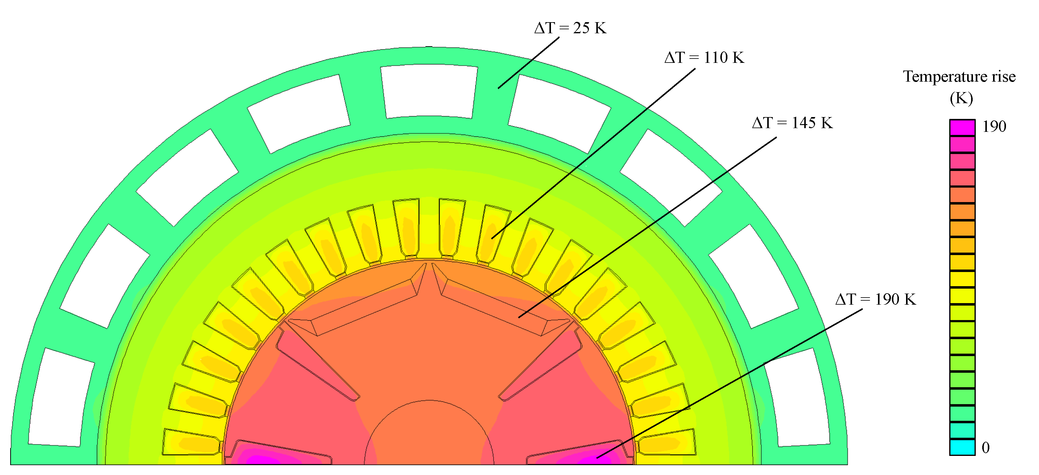
The thermal simulation proves again that the hybrid-excited motor cannot be cooled with the same strategy as an IPM motor, even though water cooling is more effective than the forced-air system adopted in the simulation described in Section 7.3. The water cooling system is more effective in the stator; the temperatures reached are similar to those observed for the IPM motor, as shown in the thermal simulation result in Figure 36. In contrast, the rotor temperatures are higher than in the IPM motor because the rotor is thermally isolated with respect to the stator. In addition, PM temperature increases can cause demagnetization (more than 140 $\mathrm{K}$), and the rotor winding maximum temperature increase reaches 190 $\mathrm{K}$.

Considering the presence of additional rotor windings, the HEPM motor cooling system has to be improved. Thus, another thermal simulation is carried out that also includes a rotor cooling system. Figure 37 shows the HEPM motor temperature increase when the rotor is cooled by oil flowing inside the shaft. To reach a maximum temperature increase of about 120 $\mathrm{K}$ in the rotor windings, the convective heat transfer coefficient is equal to $h=350\mathrm{W}/({\mathrm{m}}^2·\mathrm{K})$.

8. Conclusions

The hybrid-excitation motor is a new type of synchronous machine that includes both permanent magnets and excitation coils in the rotor.

This special type of machine requires a special manufacturing procedure. First, an additional winding has to be wrapped in the rotor. Then, a slip ring and brushes are needed to supply the excitation current. Concerning the stator winding, the two-inverter power supply system is suitable for high-power applications and allows for a redundant power source. Both inverters are designed to supply half the total required power.

Despite all the additional components, such a motor is characterized by a requirement for less magnetic material than traditional IPM motors. Designs that allow for a reduction in the need for rare-earth materials are currently a trend due to the high cost and poor availability of such materials.

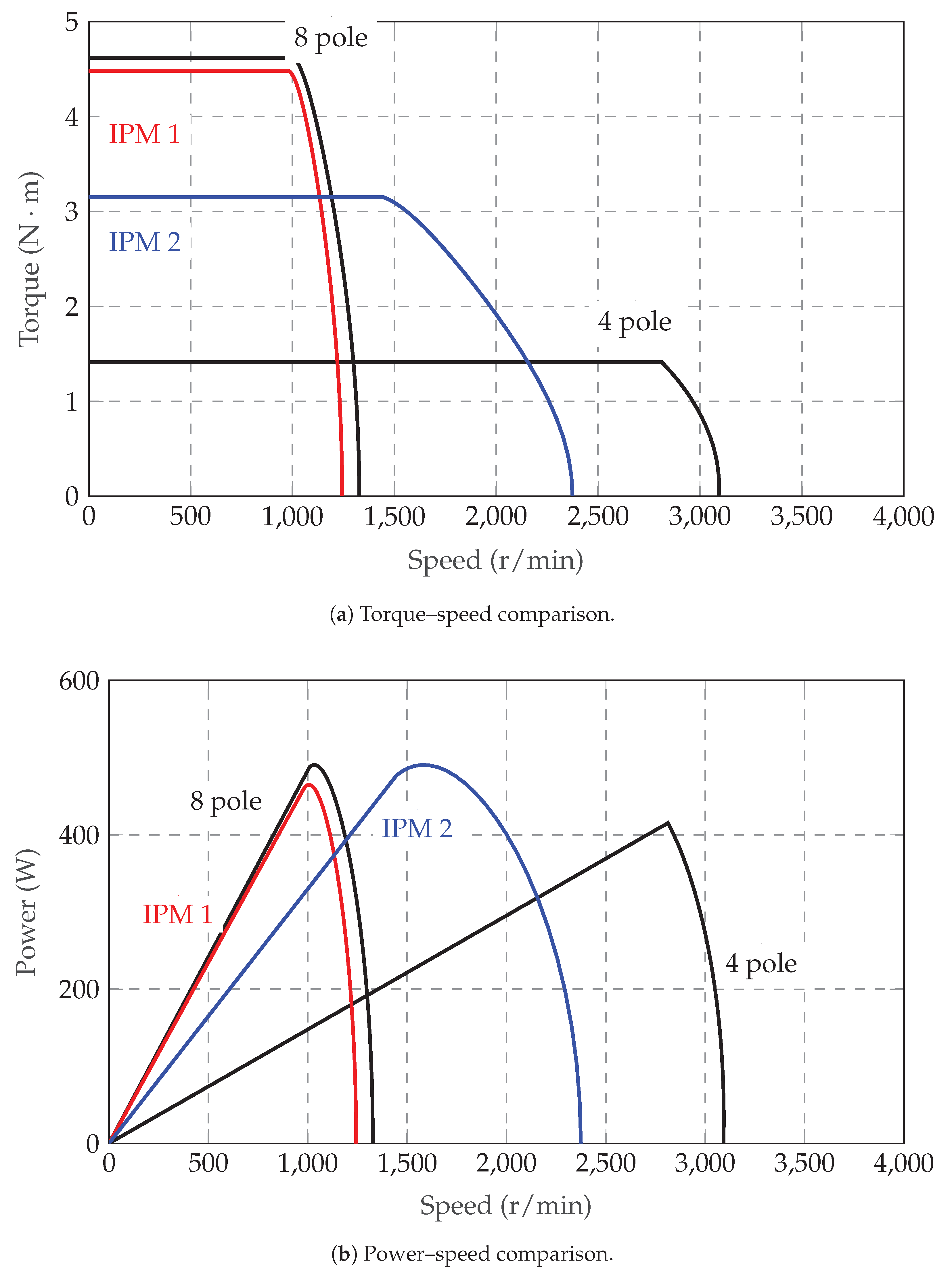
The HEPM motor with a change in polarity exhibits several advantages. Firstly, the reduced need for magnetic material is useful. In addition, other advantages are its high torque at low speeds, which is achieved by means of the eight-pole configuration, and its extension of the operating speed range, which is achieved by means of the four-pole configuration. It is also possible to modulate the flux to improve the power factor of the HE-IPM machine.

The main drawback underlined in this study is the high torque ripple. However, it is shown herein that proper strategies exist to greatly reduce it.

In addition to the electromagnetic and mechanical performance of the dual-polarity HEPM motor, its thermal behaviour is also analyzed in this work, and a possible cooling system is suggested. Comparison with a conventional IPM motor shows the need for improved heat transfer in the rotor due to the additional losses associated with the excitation coils.