Multi-Objective Parallel Machine Scheduling with Eligibility Constraints for the Kitting of Metal Structural Parts

Abstract

This paper studied a class of coupling problems of material assignment, part nesting, kit delivery and parallel machine scheduling. The aim of this paper was to solve the scheduling problem of metal structural part processing and welding assembly with eligibility constraints. A two-stage mixed-integer programming model was constructed. The eligibility constraints took into account the material type of parts and nesting. The objectives were to minimize the makespan, maximize material utilization and minimize the kit delivery metrics (kitting time and numbers of earliness and tardiness of kits). A hierarchical optimization approach was proposed. The scheduling model was solved by using the Gurobi solver in the first stage, and the results were used to constrain the second stage. The second stage of the scheduling model was solved using an improved multi-objective genetic algorithm. Due to the strong coupling relationships among the sorting of parts, the sorting of each profile and the sorting of each material, a hybrid encoding and decoding mode was designed for part sorting with eligibility constraints. Finally, the proposed scheduling approach was applied to actual production cases. The data showed that when the number of components exceeded 300 (the number of parts was about 1500), the material utilization reached 95%. Choosing a suitable number of machines, machine utilization reached 90%. The results demonstrated the effectiveness of the proposed scheduling model and algorithm.

1. Introduction

In the context of Industry 4.0, mass customization is developing rapidly, and customers can choose customized products with different configurations. Mass customization is a modern manufacturing mode that combines mass production with customization [1]. Mass customization can help balance the contradiction between order differentiation and manufacturing costs [2] and enables greater flexibility in manufacturing systems [3]. The key to achieving mass customization and rapid response is providing diverse product configurations to meet customer requirements and shortening the order delivery time [4]. It is an important way to attract customers and improve the competitiveness of manufacturing enterprises. However, it often adds complexity to the production scheduling process. Production scheduling is the core of modern manufacturing, and it aims at balancing customer requirements and manufacturing resources, as well as improving quality, increasing efficiency and reducing costs and consumption. Metal structural parts are widely used in aerospace products, ships, automobiles, transmission towers and other equipment. Generally, their production process includes part nesting, cutting processing and welding assembly. Due to the differentiation of orders, there are many types of metal structural parts and small batches, resulting in machine load imbalance, low material utilization, poor kitting and a backlog of work-in-progress in the production process.

The production process of metal structural parts could be regarded as a kind of parallel machine scheduling problem (PMSP). The classical PMSP assumes that there are n jobs, and each job must be processed by one of m parallel machines. The objectives of the PMSP are to minimize the makespan, the tardiness, etc. However, in the actual production process, part nesting makes the metal structural parts not independent. In addition, this is necessary for the close connection between machining and welding assembly. The absence of any one part leads to the retention of all the parts belonging to the same kit or component, and subsequent follow-ups cannot be carried out during assembly welding. Due to the variety of orders and the fluctuation in the price of metal materials, it is required that suitable scheduling must comprehensively consider the above factors to improve the machining and assembly efficiency of the metal structural parts and reduce the waste of materials. Therefore, eligibility constraints need to be considered, i.e., the material-type constraints of each structural part and the nesting constraints. Part nesting is necessary to optimize material utilization. When welding assembly is performed, it is necessary to ensure that all the parts of the same component or product are completed as close to the same time as possible, a process called kitting. Compared with the classical PMSP, this makes problem modeling and solution more complicated and puts forward higher requirements for the comprehensive performance of the scheduling approach.

Since McNaughton studied the PMSP for the first time [5], research on models and algorithms for the PMSP has achieved rich theoretical results [6,7]. Due to the wide range of practical applications, many researchers have focused on the PMSP in practical workshops [8,9,10]. Workshop scheduling needs to comprehensively consider the cooperation and combination of multiple production links, such as machining and assembly, making the scheduling problem more complex. Meng et al. analyzed a metal-cutting plant, considered processing times, setup times, pickup times, different delivery times and machine eligibility constraints, and addressed a bi-objective cutting parallel machine scheduling problem aiming to minimize the total makespan and the total tardiness [11]. Zhang et al. researched the integrated scheduling problem of production and delivery on parallel batch processing machines with non-identical capacities in different locations in cloud manufacturing and assumed the job release time, batch sizes, processing times and delivery times. A mixed-integer programming (MIP) model was presented to solve this problem, and the objective was to minimize the total service completion time [12]. Hatami et al. first described the distributed parallel machine and assembly scheduling problem (DPMASP) with eligibility constraints, aiming to optimize the scheduling of two manufacturing stages, namely, the production stage and the assembly stage. The production stage consisted of a set of identical factories with a set of unrelated parallel machines in one factory. In the assembly stage, the assembly machine was assigned to assemble all products. The proposed eligibility constraints indicated conditions whereby a job could only be assigned to an eligible factory. Minimizing the makespan of the products in the assembly stage was considered as the objective. The scheduling model was solved using CPLEX and Gurobi solver [13]. Amallynda et al. discussed an expansion of the DPMASP to a new parallel machine scenario and presented new meta-heuristics for scheduling problems. A set of products was manufactured through the assembly of several parts, each fabricated in the factories during the production stage. A product could be assembled in the assembly stage only after all the jobs in the production stage were completed. The objectives were to minimize the mean flow time and the number of tardy jobs [14]. The above studies addressed the PMSP of production and assembly or delivery with different optimization objectives. However, the scheduling objectives were mostly limited to part-level metrics; the focus was only on the point in time when the last job was finished, ignoring the actual duration of the jobs within the same component. The kit delivery efficiency was often overlooked, that is, the difference in the completion time of multiple parts of the same component was not considered. It has to be noted that the longer it takes to perform kitting, the more the work-in-process stock increases. For the case of kit delivery, Hsu et al. researched the customer order scheduling (COS) problem, where each order consisted of the set of jobs that had to be shipped as one batch at the same time. A new dispatching rule was proposed for COS in job shop scheduling, in order to reduce the total time it took to complete all jobs within the same order [15]. Chen et al. studied a synchronized scheduling problem of production and shipment with the objective to ensure that all products belonging to the same order were simultaneously completed (at least as close as possible). The proposed scheduling method was applied to a two-stage assembly flow shop scheduling [16]. Hu et al. developed a two-stage framework for the lot sizing and scheduling of the production activities at a kitting facility aiming to solve a kitting-specific production planning problem in a manufacturing setting [17]. According to the research background of this paper, it is also necessary to perform metal structural part nesting to improve the utilization rate of materials, which is a more realistic and complex PMSP. The part nesting problem [18,19], in general, has received increasing attention from researchers as an independent optimization problem [20,21]. However, the coupling problem of part nesting and parallel machine scheduling has rarely been considered. Some researchers studied the scheduling problem of cutting plates with parallel machines and solved it using branch and bound heuristic algorithms [22,23]. The above studies from the literature provide a basis for this paper, but there are few research studies on PMSP that simultaneously consider material assignment, material utilization and kit delivery.

In the production process of metal structural products, the complexity of the scheduling problem is determined by the differences in the ordered-product configuration and the resource constraints, making the scheduling problem a typical multi-objective optimization problem [24]. Various multi-objective optimization methods are reported in the existing literature, and we here summarize them [25,26]. (1) The weighted approach: The decision maker assigns different weights based on the importance of each objective. Multiple objectives are merged into a single-objective problem. (2) The hierarchical approach: The objectives are sorted based on their importance. Then, hierarchical solving is performed, and the optimal solution obtained in the previous level is used in the next level as a constraint. (3) The posterior approach: It aims to obtain a set of non-dominated solutions (also known as Pareto solutions). The decision maker selects an eligible optimal solution from this set of solutions. (4) The interactive approach: The decision maker expresses their preferred target value for each objective in the solution process. The overall computing mode extracts a feasible trade-off solution based on the objective equation and the decision maker’s preference. Many scholars have combined the posterior approach with meta-heuristic algorithms to solve multi-objective optimization problems. Meta-heuristic algorithms characterized by simple structure, flexibility, gradient-free information, easy implementation and a strong capability of circumventing local constraints can achieve a global optimum [27]. Currently, multi-objective meta-heuristics include particle swarm optimization [28], the immune genetic algorithm [29], the bat algorithm [30], etc. Deb K. proposed a fast non-dominated sorting genetic algorithm with elite strategy (NSGA-II) [31], which is widely used to solve multi-objective workshop scheduling problems because of its less computing time and good solution quality. Chen et al. applied the non-dominated sorting genetic algorithm to the design of non-compact flow shop scheduling and successfully solved the multi-objective optimization problem considering process connections [32]. Wu et al. designed a flexible job shop scheduling problem (FJSP) model with energy considerations in line with the production field. They invented an adaptive population non-dominated sorting genetic algorithm to solve the scheduling problem. The results showed that the proposed algorithm was efficient and powerful when dealing with the multi-objective FJSP that included energy consumption [33]. Regarding multi-objective PMSP, Zheng et al. investigated the PMSP of matching orders and factories; the objectives included minimizing the total tardiness and the extra quality of service costs, using NSGA-II to efficiently solve large-scale instances [34]. Although the designed algorithm considers the eligibility constraint relationship between orders and machines of a factory, orders are independent and non-decomposable minimum job units, which cannot solve scenarios containing kitting requirements. Liu et al. studied a complex product assembly line scheduling problem considering multi-skilled worker assignment and parallel team scheduling and took the maximum completion time and the imbalance degree of team workload as the optimization objectives. The improved strategies were proposed on the basis of NSGA-II, and a hybrid coding method considered worker assignment and task order [35]. They focused the completion time due to the worker assignment scheme but did not consider the matching relationship between workers and jobs. Therefore, the proposed approaches were difficult to be applied to the optimization problem containing the coupled material assignment and the job scheduling studied in this paper. Bandyopadhyay et al. addressed a PMSP with three objectives by improved NSGA-II. Experimental results showed that the proposed algorithm also works effectively [36]. However, this algorithm was only applied to the classical PMSP scheduling problem and could not solve the scheduling problem constrained by the material assignment and the part nesting. Therefore, current research results on multi-objective optimization algorithms applied to the production scheduling did not yet have an effective algorithm to solve the multi-objective optimization problem of production scheduling in metal structural parts for kitting delivery considering both the material assignment and the part nesting constraints, as proposed in this paper.

Due to the particularity of the production process of metal structural parts, there is still a lack of effective scheduling models and algorithms to address such complex scheduling problems. Therefore, this paper studied a multi-objective scheduling problem of the kit delivery of metal structural parts with eligibility constraints. The scheduling process was divided into two stages to solve material assignment and part nesting, as well as kit delivery for welding assembly. Aiming at solving the two-stage scheduling problem, a mixed-integer programming scheduling model with eligibility constraints was established, and a hierarchical multi-objective optimization approach was designed. Briefly, the first stage of the scheduling model was solved using Gurobi, and the results of the first stage were used to constrain the second stage. The second stage of the scheduling model was solved using an improved multi-objective genetic algorithm. Furthermore, according to the scheduling characteristics of the metal structural parts, a hybrid encoding–decoding mode with eligibility constraints was designed. Finally, the validity of the model and algorithm was verified using the production scheduling data of the metal structural parts of bus frames.

The remainder of this article is arranged as follows: In Section 2, we describe the scheduling problem and propose a mixed-integer programming model. The design of an improved multi-objective genetic algorithm to solve the corresponding scheduling model is presented in Section 3. In Section 4, we conduct a numerical study. Finally, we summarize the contributions of this paper and suggest possible directions for future research in Section 5.

2. Problem Description

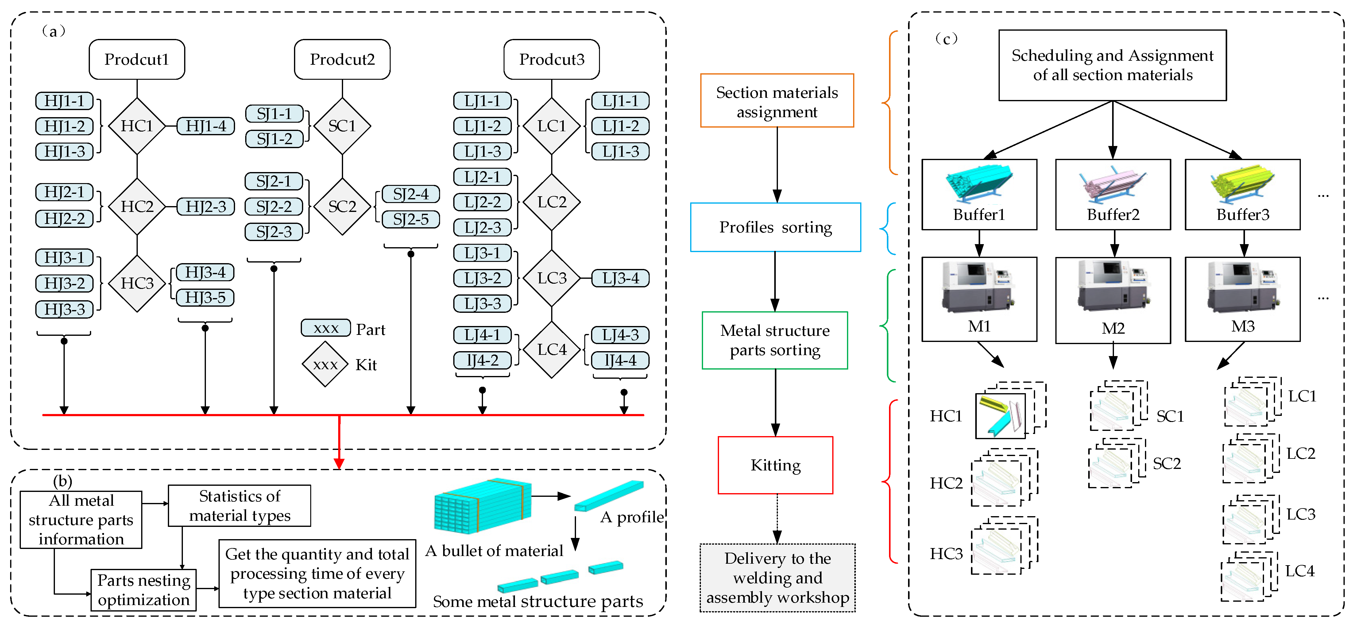
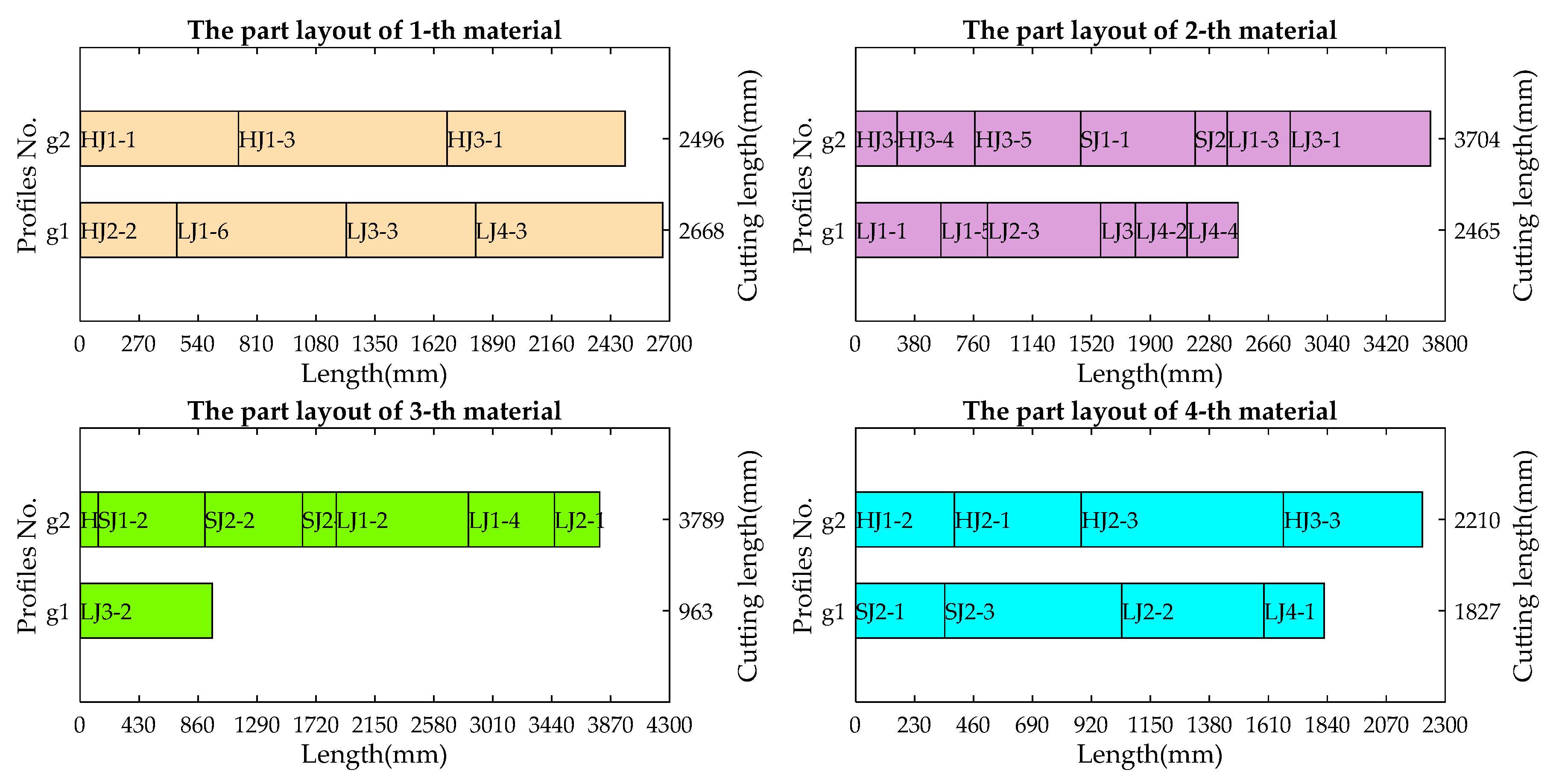
A typical product structure of metal structural parts is shown in Figure 1a. It can generally include multiple levels: parts, kits or components, and products. Welding is performed at each level to form sub-assemblies or assemblies and finally form products. Customized product configurations lead to the difference in the sub-assemblies at all the levels of the product and part processing. A machining workshop produces metal structural parts for multiple ordered products. Various types of materials are used in production. The type of a bundle of material corresponds to a cross-sectional shape and size. A bundle of material includes multiple identical profiles (the profile is a straight bar with a certain cross-sectional shape and size). All metal structural parts are cut from profiles one by one, and different parts could need to share the same material or even belong to the same profile due to part nesting. Therefore, the material type of the parts in the product and part nesting impose eligibility constraints on production scheduling. Before production, the material types of all parts are selected, and part nesting is performed to obtain the number of single profiles for each material, as shown in Figure 1b. The processing time of a single profile and the total processing time of each material are obtained based on the known processing time of the part and the results of part nesting. The production process is divided into four steps, as shown in Figure 1c: (1) each material is sequentially allocated to buffers according to its total processing time and sequence. (2) Each profile in the buffer enters the machine in sequence according to profile sorting. (3) The single profile is cut into parts in sequence according to part sorting. (4) After the parts belonging to the same kit or product undergo kitting, they are delivered to the workshop.

2.1. Notation

According to the problem description, the mathematical symbols are as follows:

Parameters:

$i$	Index of machines: $i\in M$;
$r$	Index of orders: $r\in O$;
$k$	Index of kits (or components): $k\in C_r$;
$j$	Index of parts: $j\in J$;
$h$	Index of material type: $h\in P$;
$g$	Index of profiles that belong to material $h:$$g\in P_h$;
$M$	Set of machines: $M=\{1,2,\cdots {,N}_M\}$;
$O$	Set of orders: $O=\{1,2,\cdots {,N}_O\}$;
$C_r$	Set of kits (or components) that belong to order $r:$ $C_r=\{1,2,\cdots {,N}_{C_r}\}$;
$J$	Set of parts: $J=\{1,2,\cdots {,N}_J\}$;
$P$	Set of material types: $P=\{1,2,\cdots {,N}_P\}$;
$P_h$	Set of profiles of material $h:P_h=\{1,2,\cdots {,N}_{P_h}\}$.

Input variables:

$t_j$	Processing time of part $j$;
$L_j$	Length of part $j$;
$L_h$	Length of material $h$;
$T_h$	Processing time of material $h$;
$T_{hg}$	Processing time of the $g$-th profile of material $h$;
$t_{hgj}$	Processing time of part $j$, which belongs to $g$-th profile, in material $h$;
$H$	Assumed to be a big number.

Decision variables:

$S_h$	Starting time of material $h$ in a machine;
$S_{hg}$	Starting time of $g$-th profile of material $h$;
$S_{hgj}$	Starting time of part $j$, which belongs to the $g$-th profile, in material $h$;
${SC}_{kj}$	Starting time of part $j$, which belongs to kit $k$;
${EC}_{kj}$	Completion time of part $j$, which belongs to kit $k$;
${SW}_k$	Starting time of kit delivery window of kit $k$;
${EW}_k$	Completion time of kit delivery window of kit $k$;
${\phi }_{hj}$	Equals 1 if material type of part $j$ is $h$ and 0 otherwise;
$x_{ih}$	Equals 1 if material h is processed by machine i and 0 otherwise;
${\psi }_{hgj}$	Equals 1 if part j belongs to the g-th profile of material h and 0 otherwise;
${\delta }_{kj}$	Equals 1 if part j belongs to kit k;
${\varphi }_{ij}$	Equals 1 if part j is processed by machine i and 0 otherwise;
$y_{{ihh}^{\prime }}$	Equals 1 if material h is adjacently processed before h’ by machine i and 0 otherwise;
$z_{{ihgg}^{\prime }}$	Equals 1 if the g-th profile, which belongs to material h, is adjacently processed before the g’-th one by machine i and 0 otherwise;
$w_{{ihgg}^{\prime }}$	Equals 1 if part j, which belongs to the g-th profile of material h, is adjacently processed before j’ by machine i and 0 otherwise.

2.2. Formulation

Based on the above analysis, the researched scheduling problem of manufacturing metal structural parts in this paper is detailed below.

$N_P$ types of material ($P=\{1,2,\cdots {,N}_P\}$) are to be processed by $N_M$ identical parallel machines ($M=\{1,2,\cdots {,N}_M\}$). These materials are cut into $N_J$ parts ($J=\{1,2,\cdots {,N}_J\}$) according to $N_O$ customized orders ($O=\{1,2,\cdots {,N}_O\}$). Each material h is distributed to a machine i; the processing sequence of each profile g is determined, and each part j is assigned to a profile, so that all the parts that belong to one kit can undergo kitting and be delivered as closely to each other as possible. On the basis of satisfying the related constraints, multiple scheduling objectives are optimized. These objectives include the minimization of the makespan, the minimization of the material utilization ratio and objectives related to kitting.

The relative assumptions made are listed as follows:

(1)

Excluding the transport time of material and profiles;

(2)

Each material is only transported once, and its quantity can meet the cutting requirements of all parts using the material;

(3)

After each profile is processed, the handling time of off-cut is not counted;

(4)

The cutting edge width does not count;

(5)

The processing time of all parts is known and determined;

(6)

Each part can only be processed by one machine at most once;

(7)

The processing capacity of each machine is the same;

(8)

Each machine can only process at most one part at a time;

(9)

Preemption is not allowed; that is, any started operation cannot be stopped before completion;

(10)

All parts and machines are available at the beginning; machine failures and blocks are not considered.

2.3. Scheduling Model

In this section, an extended parallel machine scheduling model is established based on multi-objective optimization. The scheduling problem is separated into two stages. The first stage is to schedule all materials onto a set of parallel production machines M. Meanwhile, part nesting is carried out to determine the part set belonging to the same profile. In the second stage, all parts are scheduled and sorted according to the eligibility constraints to obtain the optimal processing sequence of materials, profiles and parts.

In actual production, the makespan and material utilization are given priority, as they directly affect the cost of the enterprise. Then, they need to meet the requirements of kitting to guarantee order delivery. Therefore, the optimization objectives corresponding to two-stage scheduling have priority. The optimization objectives in the first stage have higher priority than those in the second stage. We propose a hierarchical optimization approach. The results of the first stage are used to constrain the second stage. Hence, it is necessary to first achieve the objectives related to the makespan and part nesting and lastly optimize the objectives related to kitting.

Based on the notation defined, we propose the mathematical model in the next sections.

2.3.1. Material Assignment

The purpose of material assignment is to minimize the makespan. This is related to the number of machines and the processing time of each material. The mathematical model of material assignment is as shown below.

$$f_1=\min \left({{\displaystyle \sum }}_{h=1}^{N_p}{T}_h{x}_{ih}\right)$$

(1)

s.t.,

$${{\displaystyle \sum }}_{i=1}^{N_M}{x}_{ih}=1(h=1,2,\cdots {,N}_P)$$

(2)

$${{\displaystyle \sum }}_{h=1}^{N_P}{x}_{ih}\ge 1(i=1,2,\cdots {,N}_M)$$

(3)

$$T_h={{\displaystyle \sum }}_{j=1}^{N_J}{t}_j{\phi }_{hj}(h=1,2,\cdots {,N}_P)$$

(4)

$$x_{ih}{,\phi }_{hj}\in \{1,0\}(\forall i\in M,\forall h\in P,\forall j\in J)$$

(5)

In the formulation, objective (1) is to minimize the maximum makespan of machines M in the first stage. Constraint (2) imposes that each material h is only processed by one machine and can only be processed once. Constraint (3) enforces that at least one material is processed on one machine. Equation (4) calculates the total processing time of material h. Constraint (5) specifies that decision variables $x_{ih}$ and ${\phi }_{hj}$ are binary.

2.3.2. Part Nesting

The material utilization is expressed as a quantity. Here, only the influence of the part length on the nesting was considered, which was a one-dimensional nesting optimization problem. Hence, to optimize the quantity of each material, the mathematical model of material h is as shown below.

$$f_2^h=\min ({{\displaystyle \sum }}_{g=1}^{N_{G_h}}\min (1,{{\displaystyle \sum }}_{j=1}^{N_J}{\psi }_{hgj}\left)\right)$$

(6)

s.t.,

$${{\displaystyle \sum }}_{g=1}^{N_{G_h}}{\psi }_{hgj}=1(\forall j\in J)$$

(7)

$${{\displaystyle \sum }}_{j=1}^{N_J}{\psi }_{hgj}{L}_j\le L_h(g=1,2,\cdots {,N}_{G_h})$$

(8)

$${\psi }_{hgj}\in \{1,0\}(\forall g\in G_h,\forall j\in J)$$

(9)

In the optimization model, objective (6) accounts for the minimization of the total quantity of material h required in the first stage. Constraint (7) imposes that each part j is only assigned to one profile g that belongs to material h and can only be assigned once. Constraint (8) imposes that the total length of parts distributed on material h cannot exceed the length of material h. Constraint (9) defines that decision variable ${\psi }_{hgj}$ is binary.

Formulas (1)–(9) above are the optimization objectives and constraints relative to the first stage. We carry out the distribution of each material and the part layout and obtain the optimal scheme. Then, we establish a mathematical model of optimization objectives related to kitting.

2.3.3. Optimization of Kitting

The second stage optimizes three evaluation indicators at the same time: minimizing the maximum kit completion time ($f_3^1$), minimizing the number of earliness kits ($f_3^2$) and minimizing the number of tardiness kits ($f_3^3$).

(1) Minimizing the maximum kit completion time: The completion time of kit k is the difference between the completion time of the last part of the kit and the starting time of the first part.

$$f_3^1=\min \left(\max \right({SC}_k-{EC}_k\left)\right)$$

(10)

$${SC}_k{=\min (S}_{hgj}{\delta }_{kj}{),EC}_k{=\max \left(\right(S}_{hgj}{+t}_j{)\delta }_{kj})$$

(11)

(2) Minimizing the number of earliness kits: Earliness kits are components whose last part’s completion time is shorter than the starting time of the kit’s delivery window. The number of earliness kits is the sum of the number of components completed ahead of schedule.

$$f_3^2=\min ({{\displaystyle \sum }}_{k=1}^{\mathrm{Cr}}{\max (0,\mathrm{sign}(SW}_k{-SC}_k\left)\right))$$

(12)

(3) Minimizing the number of tardiness kits: Tardiness kits are components whose last part’s completion time is longer than the completion time of the kit’s delivery window. The number of tardiness kits is the sum of the number of all delayed components.

$$f_3^3=\min ({{\displaystyle \sum }}_{k=1}^{\mathrm{Cr}}{\max (0,\mathrm{sign}(EC}_k{-EW}_k\left)\right))$$

(13)

s.t.,

$${{\displaystyle \sum }}_{i=1}^{N_M}{\varphi }_{ij}=1$$

(14)

$$1\le {{\displaystyle \sum }}_{j=1}^{N_J}{\varphi }_{ij}\le N_J(\forall i\in M)$$

(15)

$${{\displaystyle \sum }}_{h^{\prime }}^{N_p}{y}_{{ihh}^{\prime }}\le x_{\mathrm{ih}} (h=0,1,2,\cdots {,N}_p;h\ne h^{\prime })$$

(16)

$${{\displaystyle \sum }}_{h=0}^{N_p}{y}_{{ihh}^{\prime }}{=x}_{{ih}^{\prime }}(h\ne h^{\prime };\forall h^{\prime }\in P)$$

(17)

$${{\displaystyle \sum }}_{g^{\prime }=1}^{N_h}{z}_{{ihgg}^{\prime }}\le 1(g=0,1,2,\cdots {,N}_h;g\ne g^{\prime })$$

(18)

$${{\displaystyle \sum }}_{g=0}^{N_h}{z}_{{ihgg}^{\prime }}=1(g\ne g^{\prime },\forall g^{\prime }\in G_h)$$

(19)

$${{\displaystyle \sum }}_{j^{\prime }=1}^{N_J}{w}_{{ihgjj}^{\prime }}\le {\psi }_{\mathrm{hgj}}(j=0,1,2,\cdots {,N}_J;j\ne j^{\prime })$$

(20)

$${{\displaystyle \sum }}_{j=0}^{N_J}{w}_{{ihgjj}^{\prime }}{=\psi }_{{hgj}^{\prime }}(j\ne j^{\prime },\forall j^{\prime }\in J)$$

(21)

$$S_{hgj}{+t}_j\le S_{{hgj}^{\prime }}{+H(1-w}_{{ihgjj}^{\prime }})$$

(22)

$$S_{hg}{=S}_h+{{\displaystyle \sum }}_{g^{\prime }=1}^{g-1}{T}_{{hg}^{\prime }}$$

(23)

$$S_{hgj}{=S}_{hg}+{{\displaystyle \sum }}_{j^{\prime }=1}^{j-1}{T}_{{hgj}^{\prime }}$$

(24)

$$S_{hgj}\ge 0$$

(25)

$$T_{hg}={{\displaystyle \sum }}_{j=1}^{N_J}{t}_j{\psi }_{hgj}$$

(26)

$$S_{h(g+1)} - S_{hg} {-T}_{hg}\ge 0$$

(27)

$${\varphi }_{ij}{,y}_{{ihh}^{\prime }}{,z}_{{ihgg}^{\prime }}{,w}_{{igjj}^{\prime }}\in \{1,0\}$$

(28)

Constraint (14) indicates that each part can only be processed by one machine and can only be processed once. Constraint (15) imposes that each machine needs to process parts. Constraints (16) and (17) indicate that material h is adjacently processed before h’ by machine i. Constraints (18) and (19) denote that profile g belongs to material h and is adjacently processed before g’ by machine i. Constraints (20) and (21) indicate that two parts on the g-th profile of material h are processed one after the other by a machine. Constraint (22) indicates that one machine can only process one part at a time. Constraint (23) is used to calculate the start of the processing time of each material. Constraint (24) is used to calculate the start of the processing time of each part. Constraint (25) indicates that every part is processed. Constraints (26) and (27) indicate that all processing is non-pre-emptive and that processing cannot be interrupted once it starts. Constraint (28) specifies that the decision variables, including ${\varphi }_{ij}$, $y_{{ihh}^{\prime }}$, $z_{{ihgg}^{\prime }}$ and $w_{{ihgjj}^{\prime }}$, are binary.

3. Algorithm Design

The scheduling model consists of two stages: material assignment and part nesting constitute the first stage, and profile sorting and part processing sorting form the second stage. The two stages include three optimization models. From the perspective of the scale and computational complexity of the three optimization models, the first model is smaller than the second one, and the second one is smaller than the third one. Hence, we proposed a hierarchical optimization approach. Taking into account the accuracy and efficiency of the solution, model 1 and model 2 are solved with an accurate method that uses Gurobi as the solver in the first stage. Gurobi can solve many types of problems, including mixed-integer programming, and is the best and fastest linear programming/quadratic programming solver in the world today because of its wide range of problem types and high solution efficiency. At the same time, Gurobi can be easily integrated into third-party platforms such as MATLAB, Python or Net, and is more capable of handling a wide range in complex scientific research and applications, so Gurobi was chosen as the first-stage optimization solver. According to the solution results of the first stage, the number of profiles belonging to each material, the index of all profiles of each material and the part index of a profile can be obtained, and there is a fixed subordination relationship among them. The subordination relationships are eligibility constraints. The results of the first stage were used for eligibility constraints in the second stage. Model 3 belongs to the second stage, is a multi-objective optimization model, and the solution scale is large, so we proposed an improved multi-objective meta-heuristics algorithm based on the NSGA-II. Due to eligibility constraints, there are strong coupling relationships among the sorting of parts, the sorting of each profile and the sorting of each material. In order to express these sorting relationships, part-based coding is designed; in order to improve the problem of insufficient crossover due to too-long chromosomes, a segmented crossover method is designed. In order to improve the iterative quality of the population, the non-dominated sorting method is improved, and the elite retention strategy is used to improve the iterative quality of the population. The flow chart of the improved NSGA-II algorithm is shown in Figure 2.

3.1. Coding

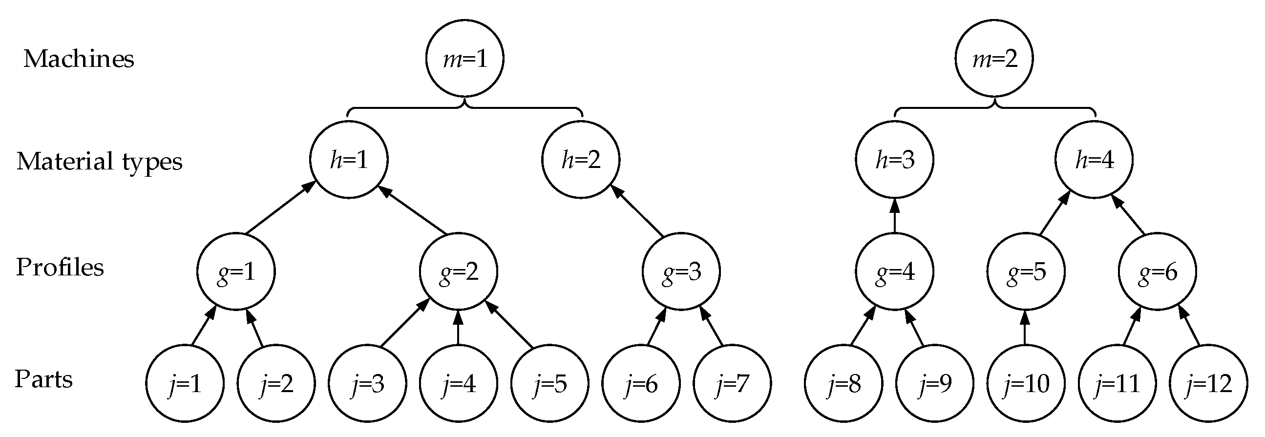
This paper designs an integer coding method based on parts that can effectively express the sorting of materials and their assignment to each machine, the order of each material among the materials and the sorting of parts and their assignment to each profile. According to the optimization results of the model in the first stage, the subordination relationships among parts, profiles, materials and machines can be obtained. This kind of affiliation can be expressed with a tree diagram, as shown in Figure 3.

First, the initial reference code is designed; this is an integer sequence $[1,2,\cdots {,N}_J]$, where N_J is the sum of the number of all parts, that is, the length of the chromosome. In the iterative process, the reference codes are reordered according to different chromosome sequences to form a feasible job code. A feasible encoding is [649251110121783]. Since all the permutations of the chromosome are merely the reordering of the original reference code, the number and type of certain elements in the reference code are not changed, nor are new elements formed. Therefore, this coding method does not generate illegal chromosomes. This coding method avoids reducing the algorithm search efficiency due to the identification of illegal chromosomes.

3.2. Decoding

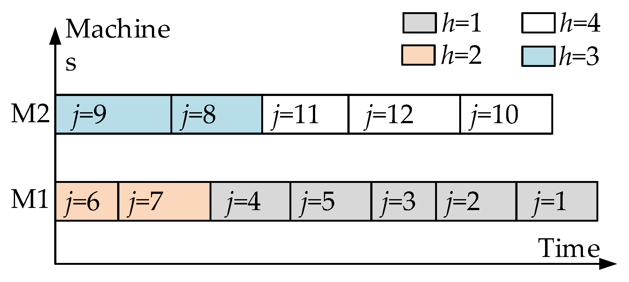
The genetic-locus value in the designed chromosome represents the part number, and the parts are sorted according to the sequence of the genetic loci. The other parts on the profile are indexed according to the part number on the genetic locus to form the processing sequence of the parts on the profile. The other profiles of the material category are indexed according to the number of profiles to form the processing sequence of the profile. The other materials on the machine are indexed according to the number of materials to form the processing sequence of materials. The decoding process is shown in Figure 4. According to the above method, the sequencing of all the genetic loci is completed to form a sequencing scheme.

Combining the processing time of parts, the processing time of each profile and the processing time of each material, a feasible scheduling plan is finally formed. After decoding according to the chromosome generated above, Gantt charts are formed for material assignment scheduling and profile cutting scheduling. Moreover, the Gantt chart of part sorting is shown in Figure 5, assuming that the first kit contains parts 1, 2, 10 and 11, the second one contains parts 3, 5, 6 and 9 and the third one contains parts 4, 7, 8 and 12. We can obtain the Gantt chart of kitting according to the Gantt chart of part sorting, as shown in Figure 6, and calculate the objective function related to the complete kit.

3.3. Fast Non-Dominated Sorting

In a multi-objective optimization problem, in order to compare the pros and cons of two individuals, two measurement indicators—the non-dominated ranking level and the crowding distance—are commonly used. If none of the goals of individual p are worse than those of individual q and at least one goal of individual p is better than those of individual q, then individual p dominates individual q. First, all individuals are ranked according to non-dominated relationships. Obviously, the individuals at the first front end are dominant, and the individuals at the second front end are dominated by the first front-end individuals. Individuals are assigned to different front ends through sorting, and for individuals at the same front end, pros and cons can be determined by comparing the crowding distance until all individuals are sorted.

The evaluation of individual fitness and selection is performed using two methods: fast non-dominated sorting and crowding distance. Each individual in the population is assigned a non-dominated rank through rapid non-dominated sorting. For the population of pop individuals, it is assumed that $n_i$ individuals are dominated by the i-th individual and that the individuals dominating others form set $s_i$. The process of rapid non-dominated sorting is described below.

Step 1: Compare the fitness values of the individuals (fitness equals objectives $f_3^1$, $f_3^2$ and $f_3^3$ ); count the number of non-dominated individuals q ($n_i=0,i\in \left\{1,2,\cdots ,q\right\}$); set these individuals to level 1 ($i_{rank}=1$).

Step 2: Determine the $s_k$ ($k\in \left\{1,2,\cdots ,q\right\}$) of each individual on level 1; judge whether the $n_{t-1}$ of each individual t in $s_k$ equals 0; set the individuals with $n_{k-1}$= 0 to level 2.

Step 3: Repeat Step 2 until all individuals are set to the corresponding rank. Then, the individuals on the same level are subjected to a fitness comparison based on the crowding distance.

The crowding distance of each individual is calculated as described below.

Step 1: Find the non-dominated individuals of the same front end and place them in a matrix W.

Step 2: Based on the c-th objective function, arrange matrix W in descending order, where c = 1.

Step 3: Let the crowding distance between the first and last individuals in matrix W be infinite.

Step 4: Calculate the crowding distance of all individuals in matrix W. The calculation formula is shown below.

$$d\left(f\right)=\frac{d(f+1)-d(f-1)}{d\left(\max \right)-d\left(\min \right)}$$

where d(max) represents the maximum value of the c-th objective function; d(min) represents the minimum value of the c-th objective function; and d(f + 1) and d(f − 1) represent the c-th objective function value of the (f − 1)-th individual and the (f + 1)-th individual after sorting, respectively.

Step 5: c = c + 1, $c\le T$; obtain the crowding distance under each objective function.

Step 6: Add the crowding distance under each objective function to obtain the individual’s final crowding distance. The greater the value of the crowding distance, the smaller the degree of individual crowding, and the better the diversity of the population.

3.4. Selection

In order to obtain better cross-offspring, a tournament selection strategy of two participating individuals is adopted. The size of the mating pool (pool = pop/2) is set; two different participating individuals, preferentially the participating individuals with the highest Pareto levels, are randomly selected to enter the parent population. When two individuals have the same Pareto level, the individual with a larger crowding distance is preferred to enter the parent population. When two contestants have the same Pareto level and the same crowding distance, the first contestant is selected. This process continues until the parent population of the pool size is selected.

3.5. Crossover/Mutation

Due to the large number of metal structural parts in the production workshop and the long chromosome length during encoding, the traditional cross-mutation method cannot obtain good results, so this paper proposes the segmented cross-mutation method.

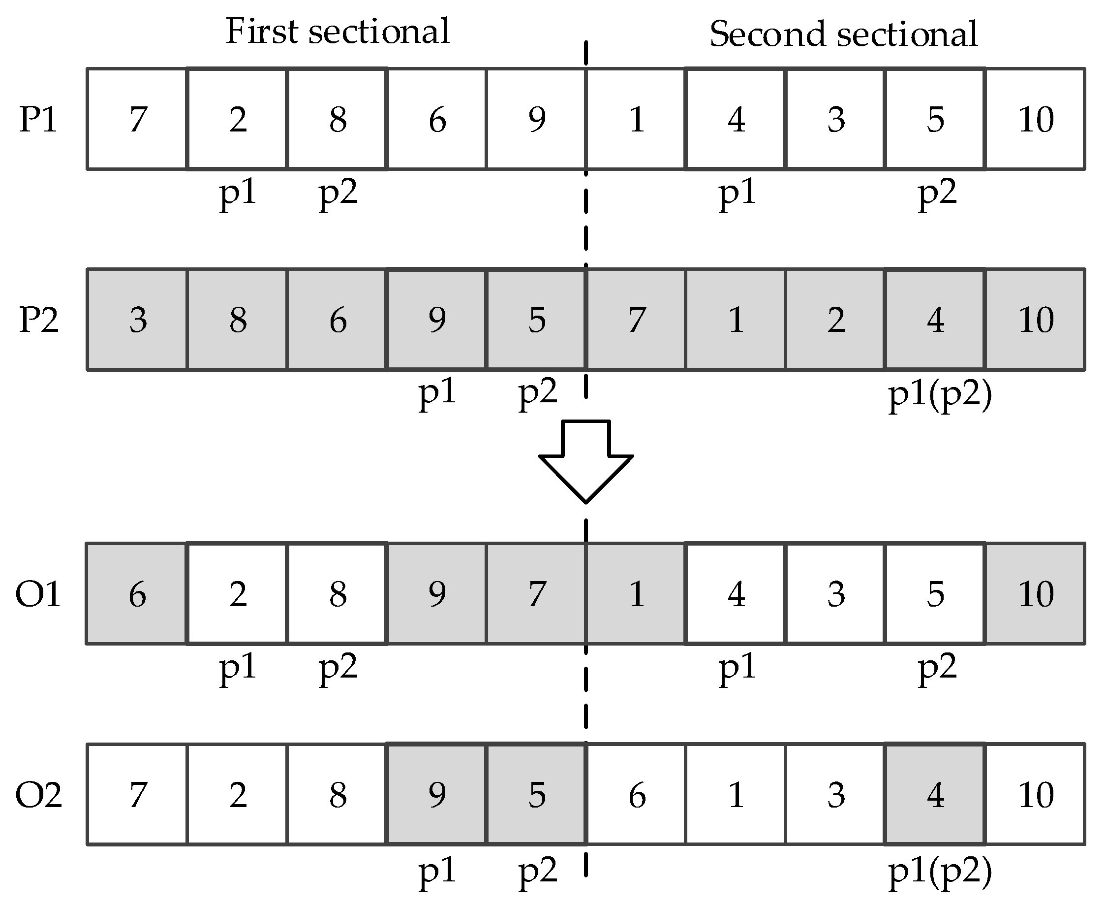
The specific crossover process of segment crossover is as follows: First, parent chromosomes P1 and P2 are segmented, the length of the segment is set to h and the chromosome is divided into x segments. Then, two genetic loci, p1 and p2, in each chromosome of the parent are randomly selected. The chromosome between loci p1 and p2 of P1 is inherited by offspring O1. Finally, the genes in P2 that are different from O1 are inherited by O1, and offspring O2 is obtained in the same way. The schematic diagram of the cross-section algorithm is shown in Figure 7.

The mutation method and crossover method in this paper use the same principle. First, the chromosomes are segmented; then, two gene positions, p1 and p2, are randomly selected in each chromosome of the parent; finally, the values of the two gene positions are exchanged. At the beginning of evolution, a larger crossover probability should be selected. This search process is conducive to maintaining the diversity of the population. In the next stage, a careful search is required to prevent the optimal solution from being destroyed and accelerate the convergence rate, and a smaller crossover probability should be selected. The adaptive crossover probability used in this article is shown below.

$$p_c{=p}_c-\frac{gen}{maxgen}{\times (p}_c-p_{cmin})$$

where p_c is the crossover probability; gen is the current number of iterations; maxgen is the maximum number of iterations; and p_cmin is the minimum value of the crossover probability.

3.6. Elite Retention Strategy

The offspring population whose population size is pop after crossover and mutation and the parent population whose population size is pooled to form a population whose size is pop + pool, and the non-dominated sorting of the combined population is performed. The Pareto level and crowding distance of each individual in the merged population are calculated, and the first pop individuals are kept as the new population obtained after iteration.

4. Computational Results

In this section, we provide the results we obtained studying a simplified real-life instance of a bus manufacturing company in China to illustrate the proposed scheduling model and the proposed algorithm. Two sets of contrasting experiments with randomly generated instances were also conducted, aiming to further evaluate the performance of the proposed algorithm. The algorithm was coded in MATLAB R2016b, and the experiments were run on an Intel Core (TM) i5-3470 3.20 GHz processor with 6.00 GB of memory in the Windows 7 operating system.

4.1. Simplified Illustrative Real Case Study

The scheduling model and the proposed algorithm were applied to customized bus orders from a bus manufacturing company. Due to the large size of the custom order, we simplified the order, aiming to verify the feasibility of the model and algorithm. In this simplified real case, the company received orders for customized buses, as shown in Figure 1a; the simplified numbers of components and parts were lower than the actual number. There were three customized bus models, product 1 (H223), product 2 (S745) and product 3 (L645). Each bus had a customized frame, which was welded together starting from some kits. The first frame consisted of three kits, the second had two kits and the third consisted of four kits. Each component consisted of a variety of metal structural parts, which were machined by machines. We used three machine tools to complete those customized tasks.

Figure 8 shows some of the metal structural parts. The complex structure, including the inclined planes, camber grooves and holes, had to be processed by a machine. The details of the corresponding input data are available in

Table 1. Order data of simplified real case.

Order (Bus Model)	Component Code	Part Code	The Length of Part (m)	Processing Time (s)	Material Data (Section/Length)
Order1 (H223)	O1-HC1	HJ1-1	0.725	13.2	Rec: 40 × 30 × 2/2.7 m
		HJ1-2	0.385	9.4	Rec: 100 × 40 × 3/2.3 m
		HJ1-3	0.955	16.2	Rec: 40 × 30 × 2/2.7 m
		HJ1-4	0.131	7.8	Rec: 40 × 40 × 2.5/4.3 m
	O1-HC2	HJ2-1	0.495	15.3	Rec: 100 × 40 × 3/2.3 m
		HJ2-2	0.443	7.8	Rec: 40 × 30 × 2/2.7 m
		HJ2-3	0.789	10.5	Rec: 100 × 40 × 3/2.3 m
	O1-HC3	HJ3-1	0.816	14.4	Rec: 40 × 30 × 2/2.7 m
		HJ3-2	0.268	16.7	Rec: 40 × 30 × 2/3.8 m
		HJ3-3	0.541	6.2	Rec: 100 × 40 × 3/2.3 m
		HJ3-4	0.501	18.9	Rec: 40 × 30 × 2/3.8 m
		HJ3-5	0.682	16.6	Rec: 40 × 30 × 2/3.8 m
Order2 (S745)	O2-SC1	SJ1-1	0.738	12.3	Rec: 40 × 30 × 2/3.8 m
		SJ1-2	0.779	11.5	Rec: 40 × 40 × 2.5/4.3 m
	O2-SC2	SJ2-1	0.348	11.7	Rec: 100 × 40 × 3/2.3 m
		SJ2-2	0.712	9.6	Rec: 40 × 40 × 2.5/4.3 m
		SJ2-3	0.69	12.6	Rec: 100 × 40 × 3/2.3 m
		SJ2-4	0.246	12.7	Rec: 40 × 40 × 2.5/4.3 m
		SJ2-5	0.207	17.3	Rec: 40 × 30 × 2/3.8 m
Order3 (L645)	O3-LC1	LJ1-1	0.549	16.9	Rec: 40 × 30 × 2/3.8 m
		LJ1-2	0.964	14.7	Rec: 40 × 40 × 2.5/4.3 m
		LJ1-3	0.406	10.7	Rec: 40 × 30 × 2/3.8 m
		LJ1-4	0.627	17.2	Rec: 40 × 40 × 2.5/4.3 m
		LJ1-5	0.301	13	Rec: 40 × 30 × 2/3.8 m
		LJ1-6	0.776	10.3	Rec: 40 × 30 × 2/2.7 m
	O3-LC2	LJ2-1	0.33	19.1	Rec: 40 × 40 × 2.5/4.3 m
		LJ2-2	0.555	18.1	Rec: 100 × 40 × 3/2.3 m
		LJ2-3	0.729	13.3	Rec: 40 × 30 × 2/3.8 m
	O3-LC3	LJ3-1	0.902	14.3	Rec: 40 × 30 × 2/3.8 m
		LJ3-2	0.963	13.8	Rec: 40 × 40 × 2.5/4.3 m
		LJ3-3	0.592	8.1	Rec: 40 × 30 × 2/2.7 m
		LJ3-4	0.225	9.5	Rec: 40 × 30 × 2/3.8 m
	O3-LC4	LJ4-1	0.234	12.1	Rec: 100 × 40 × 3/2.3 m
		LJ4-2	0.332	8.5	Rec: 40 × 30 × 2/3.8 m
		LJ4-3	0.857	17.7	Rec: 40 × 30 × 2/2.7 m
		LJ4-4	0.329	7.9	Rec: 40 × 30 × 2/3.8 m

. As the part code and component code were long, they were reported as simplified codes. The data table contains 9 components, 36 parts and 4 materials, as well as the length and processing time of each part.

Due to the priority of the optimization objectives in the first stage being higher than that in the second stage, firstly, the scheduling scheme of the first stage was optimized. Through the analysis of the mathematical model, we found that the computational scale and complexity of the first stage were much smaller than those of the second stage. Therefore, in the first stage, we used the exact method to solve the problem, and the chosen solver was Gurobi.

First, according to the order information data, the parts belonging to the same material were clustered, and the total processing time of each kind of material was obtained. The first material (L1 = 2.7 m) included seven parts, that is, HJ1-1, HJ1-3, HJ2-2, HJ3-1, LJ1-6, LJ3-3 and LJ4-3. By adding up the processing time of these parts, the total processing time of this material was calculated to be 87.7 s. Similarly, the total processing time of the second material (L2 = 3.8 m) was 175.9 s, and this material consisted of 13 parts. Moreover, the total processing times of the third (L3 = 4.3 m) and fourth (L2 = 2.3 m) materials were 106.4 s and 95.9 s, respectively.

Next, we distributed the four materials to three parallel machines. According to the principle of processing resource balance, all the kinds of materials were evenly allocated to the machines. Formulas (1)–(5) were solved with Gurobi, and the optimal result of material assignment was obtained. The scheduling Gantt chart of material distribution is shown in Figure 9. The optimal makespan was 183.6 s. The time reported in the scheduling scheme included only the part processing time, excluding other non-processing times, such as material handling, as stated in the model assumption.

Finally, we completed the part nesting with the objective of maximizing the material utilization. Using Gurobi to solve Formulas (6)–(9), we generated the result of the optimal part cutting layout, and the corresponding Gantt chart is shown in Figure 10. Two-piece profiles were used for each material, and the parts to be machined were displayed on each profile. The optimization results tried to satisfy the maximum utilization ratio of each profile, unless the parts were not enough to fill the whole profile. We calculated the utilization rate of each profile according to the Gantt chart. The average utilization rate of materials was 80.2%.

We could infer that the optimization results of the first stage could be further improved with the increase in the number of parts, that is, the larger the scale of the scheduling is, the more obvious it is. On the basis of the scheduling scheme in the first stage, we optimized the scheduling in the second stage and used the improved multi-objective algorithm to solve Formulas (10)–(28). We set the appropriate algorithm parameters of improved NSGA-II. Through optimization, we obtained the iterative convergence curve, as shown in Figure 11. The iterative curve showed that the completion time of kits, the number of kits obtained in advance and the number of delayed kits were significantly reduced. Finally, we converged to the optimal solution or near-optimal solution. The minimum completion time of kits was 131.2 s. None of the kits were completed in advance, and there were two kits that were delayed.

The part scheduling Gantt chart is shown in Figure 12, and the minimized makespan of the machine was 106.4, corresponding to machine M2. Taking machine M2 as an example, parts LJ3-2, LJ1-2, LJ1-4, SJ2-4, LJ2-1, HJ1-4, SJ1-2 and SJ2-2 were continuously processed. Combined with the results of material distribution and part layout, that is, Figure 9 and Figure 10, we could infer that the first part (LJ3-2) belonged to the first profile (g1) of the third material and that the latter six parts belonged to the second profile (g2).

The kit scheduling Gantt chart is shown in Figure 13. It can be seen from the Gantt chart that the kit completion time distribution was between 115.3 and 183.6 s. The red boxes indicate the delivery time windows in this chart. It can be seen from the figure that no kits were completed ahead of schedule and that kits C1 and C3 were delayed. The rest of the kits were completed within the due-date windows.

4.2. Randomly Generated Instance Studies

In order to further validate the effectiveness of the proposed approach for solving large-scale cases, the application validation of large-scale cases was required. Therefore, a large number of simulation cases in different scales were constructed and studied with reference to characteristics of the real case data. In these tests, we utilized the method of generating random instances designed by Olivier Holthaus [37]. There were two sets of randomly generated examples to evaluate the performance of the proposed algorithm. The input variables, including the number of parts, the processing time, the lengths of the parts and types of materials, were randomly generated with a uniform distribution. Each instance was studied, and the detailed data are shown in

Table 2. Computational results for small-size instances.

The Number of Components	The Number of Machines	Objectives of Kitting
C	M	$f_3^1$	$f_3^2$	$f_3^3$
20	5	226.3	5	2
	6	130.2	4	4
	8	139.8	3	6
40	5	390.4	25	10
	6	266.5	14	13
	8	276.7	13	13
50	6	439.8	18	22
	8	369.5	14	23
	10	298.7	13	22
60	6	584.5	26	21
	8	468.	26	18
	10	384.5	19	27
80	6	637.8	36	36
	8	567.3	20	43
	10	570.3	23	44

and

Table 3. Computational results for large-size instances.

The Number of Components	The Number of Machines	Objectives of Kitting
C	M	$f_3^1$	$f_3^2$	$f_3^3$
100	10	474.1	52	29
	12	518.6	30	54
	15	459.5	40	48
	18	351.3	38	46
	20	368.4	30	45
200	10	1200.4	91	96
	12	931.1	89	87
	15	717.4	96	74
	18	752	97	67
	20	805.1	70	99
300	10	1948.1	122	160
	12	1503.7	142	134
	15	1489.9	101	164
	18	1165.8	108	157
	20	1009.6	118	156
400	10	2351.3	209	176
	12	1834.9	214	155
	15	1653.9	181	189
	18	1454.7	151	212
	20	1501.7	119	253
500	10	3168.2	231	251
	12	2325.2	273	212
	15	1958.1	243	221
	18	2193.8	116	359
	20	1791.6	201	258

. For the first example, the set of small-size instances, the range of kits was (20, 80). For the second set of large-size instances, the numbers of kits were set as 100, 200, 300, 400 and 500. The number of parts belonging to the same component was randomly generated from a uniform distribution of (2, 8) pieces. The processing time of each part was randomly generated in the range of (5, 20) s. The length of each part was randomly generated in the range of (0.2, 1) m. The number of types of materials was randomly generated in the ranges of (10, 15) (small sized) and (15, 30) (large sized). The length of each type was randomly generated in the range of (2, 5) m. The material type of each part was randomly selected from the type set. The number of machines in each example is as shown in Table 2 and Table 3.

For each group of kit and machine, 10 random instances were generated; then, the average values of 10 tests were calculated and recorded. When the numbers of kits were set as 300, 400 and 500, the algorithm had to run for a long time to find a feasible solution. Thus, considering the feasibility of the experiment, only five random instances were generated in such a group of tests. All the average values are reported in Table 2 and Table 3.

Similar to the solving process in Section 4.1, we firstly optimized the first stage of each instance. When the kits were less than 200, the scale of Gap of the Gurobi solver was 1 × 10⁻⁴ and MIPGapAbs was 1 × 10⁻⁶. When the kit number was larger than 200, in order to improve the computational efficiency, Gap was 1 × 10⁻² and MIPGapAbs was 1 × 10⁻⁴. The statistical results are shown in Figure 14, and they fully reflect the effect of scale on production costs (that is, machine utilization and material utilization) in the first stage. The machine utilization and the material utilization presented in the experimental results were the optimization results obtained under the conditions of the used example data. The utilization ratio of materials gradually increased with the increase in the calculation scale. The utilization ratio of materials in all examples was more than 70%. When the number of kits was greater than 300, that is, the number of parts was greater than about 1500, the utilization ratio of materials was about 95%. This was due to the increase in the number of parts, making it easier for each profile to be filled and causing less off-cut. The material utilization was related to order size and part size. If the order size increases and the part size is appropriate, the proposed solution may result in the higher material utilization. From the point of view of machine task balance, the machine utilization was more than 60%. Meanwhile, we found that under the condition of the same number of components, for small-size instances (that is, the number of kits was smaller than 100 or the number of parts was smaller than 500), the machine utilization decreased with the increase in the number of machines. However, for large-size instances, the utilization increased at first and then decreased with the increase in the number of machines. Thus, the machine utilization was related to the order size and the number of machines. As shown in Figure 14, when there are 40 components and 5 machines, the machine utilization has reached 99.04%. However, the decision maker needs to consider the machine utilization and the material utilization together and choose a compromise set of optimized results. Through the analysis of the above trend, production managers can reasonably choose the number of machines according to the number of orders, so as to obtain appropriate utilization ratios of machines and materials. For example, if the number of kits was 200 or the number of parts is about 1000, 12 machine tools or 15 machine tools could be selected for processing. The machine utilization and material utilization would be 93.74% and 91.05%, if the number of machines was 12. If the number was 15, their utilization ratios would be 93.72% and 90.66%, respectively.

Secondly, on the basis of the optimization results of each first example, we obtained the results of the second stage. The statistical results of small-size instances and large-size instances are listed in Table 2 and Table 3, respectively. The data showed that the kit completion time and the numbers of earliness and tardiness of kits in each example were reduced. However, we also found that the optimization results were not obvious, especially the number of earliness and tardiness of kits. As the size in the example increased, they accounted for a maximum of nearly 50% of all processed kits. Because optimization was completed on the basis of the first-stage results, each material was scheduled in a single batch, not in batches. As a result, the parts belonging to the same kits were distributed on different profiles or materials, resulting in not being processed closely together, resulting in a longer kit completion time and an unsatisfactory number of components.

Finally, we analyzed the solution time of each example in the two stages. As shown in Figure 15, it was found that with the increase in the size of the instance, the solution time of the first stage was correspondingly prolonged, but compared with that of the second stage, the solution time was significantly reduced. Therefore, from the point of view of solution efficiency, the feasibility of our scheduling model was verified, that is, the exact method was used in the first stage, and the approximate algorithm was used in the second stage. Although the accuracy of the solution was reduced in the second stage, the calculation time was improved, and satisfactory results were obtained at the same time.

5. Conclusions and Prospects

Aiming at the problem of the machining and delivery of metal structural parts with eligibility constraints, this paper proposes a complex multi-objective parallel machine scheduling approach that considers part nesting, material assignment and kit delivery. The proposed scheduling problem is divided into two stages: In the first stage, parts are laid out, and the materials are allocated to the machines. The optimization objectives are to maximize the utilization of materials and minimize the total makespan. The second stage sorts the profiles and parts and assigns them to each machine with the objectives of minimizing the kit delivery metrics (kitting time and the numbers of early and tardy kits). A mixed-integer programming model with eligibility constraints is established, and a hierarchical optimization method is proposed. The scheduling results of the first stage are used as the constraints of the second stage. Gurobi is used to obtain the first-stage optimization results; the multi-objective genetic algorithm is improved for the second-stage scheduling optimization. The algorithm includes encoding, decoding, fast non-dominated sorting and genetic operations, and a design considering eligibility constraints is employed. To verify the model and algorithm, we used the actual production data of a metal structure workshop of bus frames. In order to further verify the scalability of the proposed scheduling method, a larger-scale scheduling optimization was conducted through the derived simulation examples. The data showed that with the increase in the number of components, the utilization rate of materials gradually increased. When the number of components exceeded 300—that is, when the number of parts exceeded about 1500—the material utilization rate reached 95%. By selecting the appropriate number of machines, the machine utilization rate reached 90%. The results verified the effectiveness of the scheduling model and algorithm proposed in this paper.

In the future, we aim to focus on extending the method proposed in this paper to more complex scheduling problems, continuing to add some practical constraints not considered in this paper, such as transit time, setup time, uncorrelated parallel machines, batch setup, integrating geometrical shape constrained for part nesting, etc., to formulate a new mathematical model for the scheduling problem of metal structural parts. Dynamic events of machine failures and order changes should also be considered. In addition, the multi-objective genetic algorithm should continue to be improved for scheduling problems, and the performance of the algorithm should be further improved by incorporating a new genetic operation mechanism.