A Novel Dynamic Cooperative Traffic Control Algorithm for the Reduction of Traffic Delay

Abstract

One of the most serious and worsening problems in much of the world is traffic congestion, which represents an undoubted menace to the quality of urban life, including wasting of time, and environmental pollution. Therefore, this study proposes a new dynamic cooperative traffic control algorithm based on Vehicle-to-Infrastructure connections to solve this problem. The proposed model contains three parts. First of all, when each vehicle enters the communication zone, it sends its estimated range of arrival time to the control center in the intersection; then the optimal passing sequence is calculated in the control center by dynamically grouping the compatible trajectories with the respect of the related safety constraints; finally, each vehicle optimizes its appropriate speed profile based on the given optimal time and speed to enter the intersection, which is sent by the control center. Several simulation cases are executed for different traffic volumes, whose results prove that vehicles under the proposed algorithm can pass the intersection with less travel time compared with traditional traffic control methods and other algorithms. Therefore, the proposed method can reduce the time delay and improve traffic efficiency.

1. Introduction

Every year, people lose lots of time due to traffic congestion in cities [1]. The intersection is one of the places where traffic jams occur frequently, because the total number of vehicles increases significantly and it is more and more expensive to extend the existing road. Therefore, many researchers attempt to find a more advanced traffic control strategy in the intersection to improve traffic efficiency and to reduce the time delay. The Intelligent Transportation System (ITS) services with the technical development of the wireless connection offer one of the possible solutions. The ITS makes it possible that the intersection can exchange information with the vehicles in real time by using vehicle-to-infrastructure (V2I) communication. As a result, the traffic control can be modeled in numerous novel ways to reduce the time delay. Next, several related traffic control models are presented.

For the first model [2,3,4], the authors assume that all the vehicles have to stop before the intersection as fast as possible due to the safety constraints and wait for the right-of-way. The control center receives the information from the vehicles by the V2I and optimizes the passing order for all the vehicles before the intersection to minimize the evacuation time. At last, the right-of-way is distributed to each vehicle respectively. The shortcoming of this model is that all the vehicles have to stop before the intersection, which wastes lots of time.

For the second model [5,6,7,8,9,10], when the vehicle enters the communication zone, it receives the schedule via V2I from the signalized intersection with fixed time control. Then the vehicle adjusts its speed profile to avoid needless deceleration before the intersection. The weakness of this model is that the traffic is under fixed time control and based on the parameters of phase and green period. As a result, it is possible that the green time is given to the lane without any traffic demand, but some vehicles wait on other lanes with the red light, which leads to the waste of green time.

Therefore, comparing with the existing intersection control approaches with V2I communication, the scientific contribution of this work focuses on the combination of above V2I model types to achieve better performance, as follows:

• When the vehicles enter the communication zone, they send their arrival time ranges to the intersection, instead of the stop time;
• Then the control center optimizes the passing sequence by dynamically grouping the lanes, rather than the fixed time control method;
• At last, the vehicles plan their speed profiles to meet the given sequence.

The proposed method in this paper is based on the following assumptions:

• all the vehicles run with the maximal speed before entering the communication zone,
• this model does not consider pedestrians,
• all vehicles are autonomous,
• there is no time delay in the V2I connection.

The paper is organized as follows: Section 1 introduces different traffic control models for the intelligent transportation system; Section 2 describes the framework of an isolated intersection, objective under the safety constraints, and the cooperative structure between the intersection and vehicles; Section 3 presents the optimization of the passing sequence with heuristic algorithm; and Section 4 shows the comparison of simulation results. Section 5 concludes the proposed novel Dynamic Cooperative Traffic Control algorithm (DCTC) and gives some research points for the future.

2. An Isolated Intersection Model

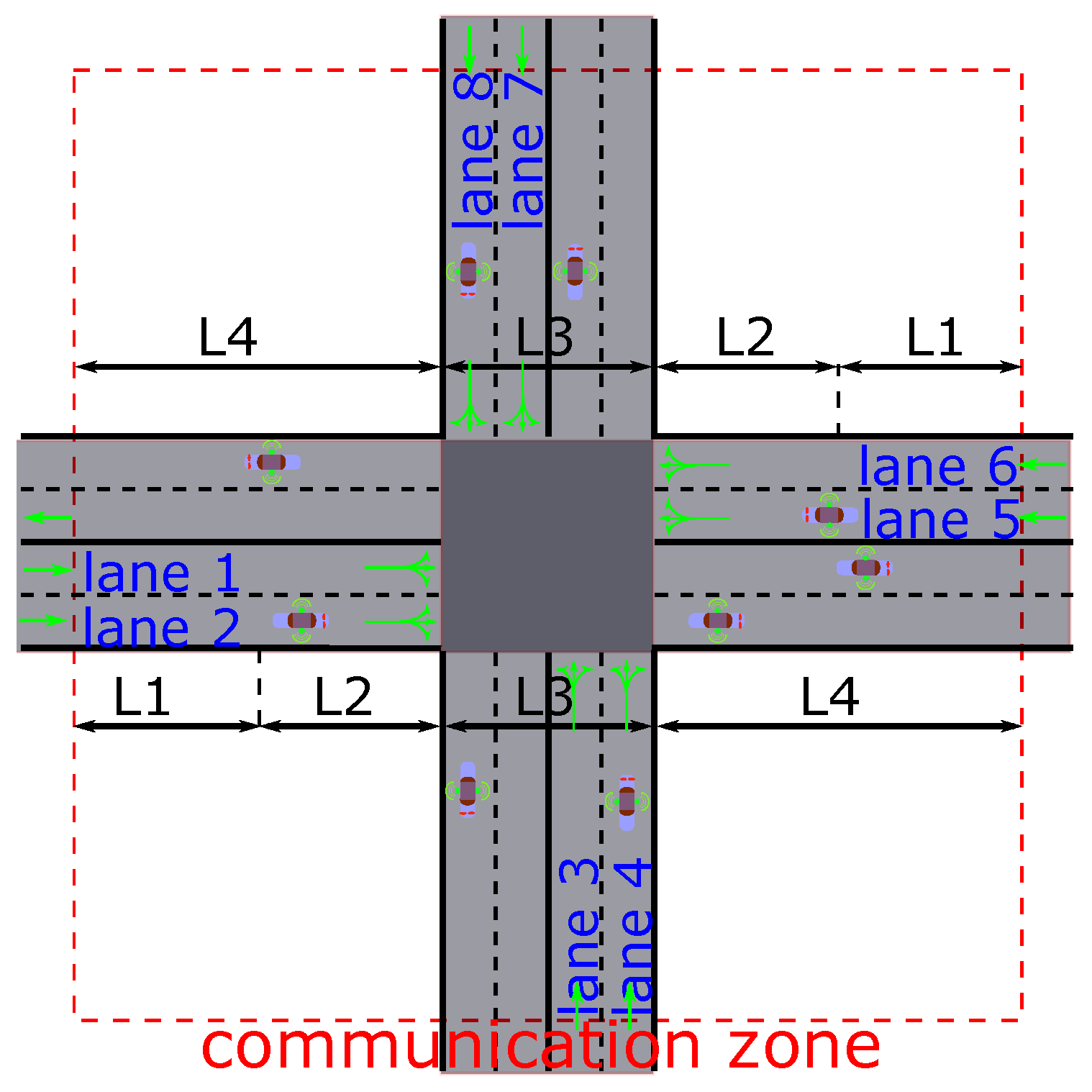
An isolated intersection model without a traffic light is shown in Figure 1 (notations are defined in the

Table 1. Notations definition.

Notations	Definition
$I_{app}$	Index of approach, $I_{app}\in [0,3].$
$I_l$	Index of lane in each approach, $N_l\in [0,1]$.
$I_m$	Index of the vehicle’s operation in the intersection.
l	Index of entrance lane, $l\in [1,8]$.
$N{V}_l$	Total number of new vehicle in the first segment L1 of the lane l.
$N_{SS}$	Total number of swap operator in each swap sequence for the evolution.
$(j,l,p)$	Subscript, the jth vehicle on lane l locates in the pth position in the passing sequence, $j\in [1,N{V}_l]$.
a, f	Superscripts, actual value and the free-flow value, respectively.
s	Sth section in the communication zone, $s\in [1,4]$.
$ETs$	Entrance time to sth section.
$EVs$	Entrance speed to sth section.
$TTs$, $TT$	Travel time in sth section. The travel time in all sections: ${\displaystyle TT=\sum _{s=1}^{4}TTs}$.
$TD$	Time delays for the entire trip.
$HW$	Headway between two successive vehicles on the same lane.
$Ls$	Length of sth section.
$Amax,Dmax$	Maximal acceleration and deceleration for each vehicle.
$Vmax,Vmin$	Maximal and minimal velocity before the intersection.
$VIma{x}_{I_m}$	Maximal allowed speed in passing the intersection according to the vehicle’s operation $I_m$.

), where there are four approaches. Each approach contains two input lanes. Each lane can be used by the vehicle to turn left, turn right, or go straight to pass the intersection. The red dotted square shows the communication zone between the vehicles and the intersection based on the V2I communication. Once the vehicle enters this zone, it can exchange information with the control center. Therefore, each vehicle can be processed respectively and can get the right of way independently. According to the movement of the vehicle, the communication zone is divided into four segments. The first and second parts (L1 and L2) are located before the intersection. The third section L3 is in the intersection. The fourth segment L4 is the remainder of the communication zone.

The objective of this work is to minimize the total time delay, which can be achieved by optimizing vehicles’ passing sequence in the intersection. A sequence means a strict order for the vehicles to pass the intersection. The formulation of the objective is shown with the Equation (1). The time delay for each vehicle is defined as the travel time difference between the real-state and the free-flow state, as the Equation (2) shows. The real-state means that the vehicle should finish the entire trip under the influence of other surrounding vehicles and intersection. The free-flow state signifies that the vehicle can accomplish all the trip with the maximal allowed speed without being disturbed by other objects. Therefore, the smaller the time delay, the faster the vehicle can complete the journey in real traffic conditions.

$$Objective:min{\displaystyle \sum _{l=1}^8\sum _{j=0}^{N{V}_l}T{D}_{(j,l,p)}}$$

(1)

$$T{D}_{(j,l,p)}=T{T}_{(j,l,p)}^a-T{T}_{(j,l,p)}^f$$

(2)

Next, the safety constraints for the above objective are presented. For each vehicle, the constraints come from the risk of collision with other vehicles in the sequence. Therefore, in order to avoid collision, a minimal time interval is imposed between the vehicles from the incompatible trajectories or from the same approach in the sequence, because there is no traffic light in the intersection and the right of way is allocated to each vehicle independently.

A trajectory means a path followed by the vehicle to finish its trip. All the trajectories in the intersection are illustrated in Figure 2. Two trajectories are defined as incompatible streams when they overlap in the intersection, because vehicles from incompatible streams may create collision accidents by passing the intersection at the same time, and vice versa.

Table 2. Conflict points among all the trajectories.

${\mathit{I}}_{\mathit{app}}$			n ($\mathit{n}\in [0,3]$)
	${\mathit{I}}_{\mathit{l}}$		0			1
		${\mathit{I}}_{\mathit{m}}$	0	1	2	0	1	2
$(n+0)mo{d}_4$	0	0
		1				◯
		2				◯	◯
	1	0		◯	◯
		1			◯
		2
$(n+1)mo{d}_4$	0	0	◯	◯		◯
		1	◯	◯	◯	◯	◯
		2
	1	0	◯	◯		◯	◯
		1	◯	◯	◯	◯	◯	◯
		2
$(n+2)mo{d}_4$	0	0		◯	◯	◯	◯
		1	◯			◯
		2	◯			◯
	1	0	◯	◯	◯	◯	◯	◯
		1	◯			◯
		2				◯
$(n+3)mo{d}_4$	0	0	◯	◯		◯	◯
		1	◯	◯		◯	◯
		2		◯			◯
	1	0	◯	◯		◯	◯
		1		◯		◯	◯
		2					◯

summarizes the incompatible points on all the approach n ($n\in [0,3]$), where the red circle ◯ indicates an incompatible relation. A trajectory can be expressed by the notation $Tra=(I_{app},I_l,I_m)$, where $I_m=0,1,2,$ means left turn, right turn, and going straight, respectively. For example, $Tra=(0,0,0)$, means that a vehicle from the lane 0 in the approach 0 will turn left in the intersection, and the notation $Tra◯Tr{a}^{\prime }$ means that the trajectories $Tra$ and $Tr{a}^{\prime }$ are incompatible.

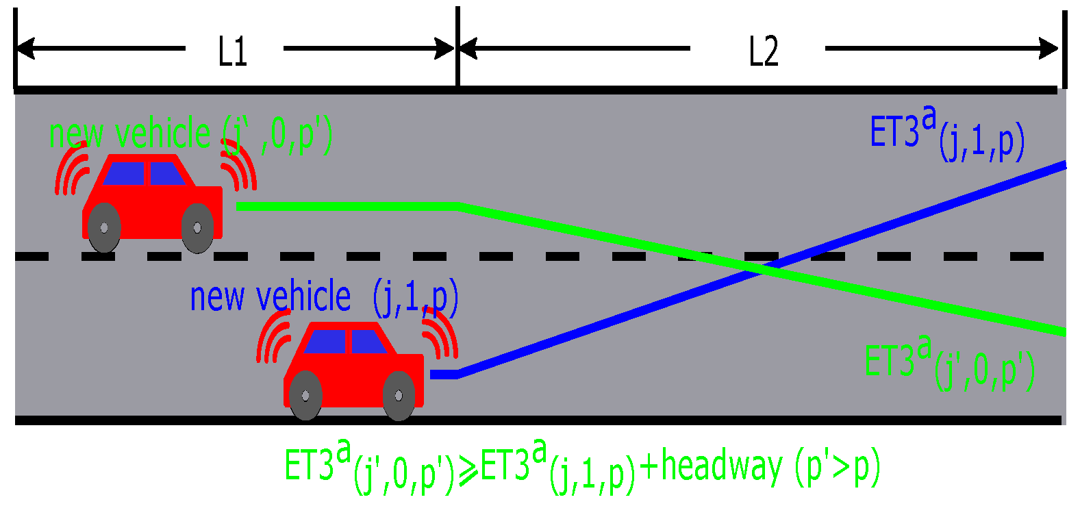
A minimum safety time should be considered for vehicles from incompatible and compatible streams on the sequence segmentation. On the one hand, for the incompatible stream, one vehicle is allowed to pass the intersection only if vehicles from an incompatible stream have passed the intersection completely. On the other hand, for the compatible stream, the safety constraints include two parts. The first part is the headway for the vehicles on the same lane. The second part means the headway for the operation of lane change, as shown in Figure 3. Therefore, the final safety time on the sequence segmentation should be the maximum value of the above three headway, as shown in the Equation (3).

$$\begin{array}{c}\hfill ET{3}_{(j,l,p)}^a=max\left\{\begin{array}{c}ET{3}_{(j,l,p)}^f\hfill \\ max(ET{3}_{(j^{\prime },l^{\prime },p^{\prime })}^a+TT{3}_{(j^{\prime },l^{\prime },p^{\prime })}^a)\hfill & \hfill l^{\prime }\begin{array}{c}\hfill ◯\end{array}l,p^{\prime }<p(l^{\prime }\in [1,8])\\ ET{3}_{(j^{\prime },l^{\prime },p^{\prime })}^a+HW\hfill & \hfill l^{\prime }=l,j=j^{\prime }+1,p^{\prime }<p\\ ET{3}_{(j^{\prime },l^{\prime },p^{\prime })}^a+HW\hfill & \hfill lanechangemode\end{array}\right.\end{array}$$

(3)

The cooperation of the proposed model is reflected by the structure that the control center optimizes the passing sequence based on the arrival information of vehicle and the vehicles plan their speed profiles before the intersection to meet the sequence. Therefore, the communication zone before the intersection is divided into two parts. The first part $L1$ is used by the control center to collect the information from the vehicle in order to optimize the passing sequence. The second part $L2$ is applied for the vehicle to modify the speed profile according to the given sequence from the control center. As a result, only the vehicles in the first part $L1$ from all the approaches are the objects to be optimized in each optimal operation. An optimal operation is defined as one process of optimizing the passing sequence. If some new vehicles enter the communication zone before the end of the previous passing sequence, the intersection control center should launch a new optimal operation without considering the vehicles which have already received the right of way. This rule’s objective is to avoid an emergency braking by the drivers. The following steps summarize the above cooperative processes, which are also illustrated with Figure 4 and Figure 5.

• When the vehicle enters the communication zone, it exchanges information with the control center and is marked as a new vehicle. The vehicle keeps the maximal speed in the $L1$ to wait for the right-of-way;
• Once a new vehicle from any approach arrives at the edge of the $L2$, an optimal operation is activated. The control center optimizes all the new vehicles in the $L1$ zone to get the passing sequence. Then, all the vehicles are marked as old vehicles. Based on the optimal sequence, the control center can calculate the allowed time $ET{3}^a$ of entering the intersection with the speed $EV{3}^a$ for each vehicle (refers to the Section 3.3) and send it to the vehicle;
• In the $L2$, there is at least one speed profile satisfying the given $ET{3}^a$ and $EV{3}^a$, because the control center optimizes the passing sequence based on the vehicle’s arrival time range in the intersection;
• In the $L3$ and $L4$, the vehicle accelerates to the maximal speed with the maximal acceleration and keeps the maximal speed to minimize the travel time.

Problem Complexity Analysis

One of the major difficulties to achieve the cooperative control in real time is the problem complexity, because the optimal control algorithm needs to consider each vehicle individually [2]. The number of all the feasible sequences is given and proved as the following Proposition.

Proposition 1 .

for an intersection of L-lane with dynamic direction combination and lane change operation, the ordered sequences of vehicles is exactly as Equation (4).

$$\begin{array}{c}\hfill \frac{\left({\sum }_{l=1}^{8}N{V}_l\right)!}{{\prod }_{I_{app}=1}^4\left({\sum }_{I_l}^{2}N{V}_{I_l}\right)!}\end{array}$$

(4)

Proof. 

There are $N{V}_i$ new vehicles on the first segment of lane i, and the intersection contains L lanes. The total number of new vehicles is found by Equation (5).

$$\sum _{i=1}^{L}N{V}_i$$

(5)

$$\left(\sum _{l=1}^{8}N{V}_l\right)!$$

(6)

Therefore, mathematically, the total possible sequences is equal to Equation (6). However, all the vehicles from the same approach obey the rule “first in first out”. Therefore, finally, it can be concluded that the total number of all feasible sequences is equal to Equation (4).

It is observed that the problem complexity sharply increases with the number of vehicles. Thus, the exhaustive search algorithm could not always find the optimal solution in a reasonable computation time. Therefore, some valuable theories in combination optimization could be applied to deal with the above complicated problem. The work [11] has successfully used the Branch and Bound algorithm to optimize the traffic control in a simple intersection. Even the above algorithm can be extended easily to control any layout of intersection. However, the computing time will increase significantly, when the geometries of intersection become more complex. Therefore, the traffic control strategy with exact algorithm can not to fulfill the real-time requirement in a large network. That argues for the application of meta-heuristics based algorithm that has very remarkable performance in solving complex NP hard problem with short calculation time. Therefore, in this work, the Artificial Bee Colony (ABC) is applied to solve the problem [12].

3. Proposed Optimization Method

The Artificial Bee Colony algorithm was proposed by Karaboga in 2005 [12]. This section presents the method of applying the ABC to find a near-optimal sequence based on the objective of time delay with reasonable calculation time. The ABC algorithm solves the optimal problem by imitating the bees’ behavior to find the nectar source. Therefore, the ABC can be used to search the optimal solution by treating the passing sequence as the nectar source. In this section, firstly, the method of coding each solution is presented. Then the swap operator process is described, which is applied as the evolution method for the ABC [13]. Next, the fitness function for each solution is shown. At last, the total process for the ABC is summarized.

3.1. Code of Sequence

The method of coding each sequence is based on the vehicle’s approach of entering the communication zone instead of its identity. It is assumed that all the vehicles from the same approach obey the rule of “first-in-first-out”. In other words, vehicle overtaking is forbidden, and all the vehicles from the same approach enter the intersection with the same order of entering the communication zone. If two vehicles from different lanes in the same approach enter the communication zone at the same time, the one from the lane 0 is ranked before the vehicle from the lane 1 (or reverse) in the sequence. The objective of this operation is to transform the code of sequence from the identity of vehicle to its approach. As a result, an illegal solution can be avoided in the operation of evolution and all the new random sequences are always legal. Then, the formulation of coding each source is presented in the Equation (7). For example, the 

Table 3. Example of coding the passing sequence in the intersection.

S	Sequence
	$\mathit{veh}\mathbf{1}$	$\mathit{veh}\mathbf{2}$	$\mathit{veh}\mathbf{3}$
001	1	2	3
010	1	3	2
100	2	3	1

shows all the possibilities of the sequence, when there are only three vehicles in the intersection. The $veh1$ enters the communication zone before the $veh2$ from the same approach 0 and the $veh3$ comes from the approach 1. For instance, the first row in the Table 3 ($S=001$) means the passing sequence ($veh1$, $veh2$, $veh3$) for all the vehicles.

$$\begin{array}{c}\hfill S=\{I_{app},I_{app}^{\prime },\dots \dots \}\end{array}$$

(7)

3.2. Swap Operator Process

Each Swap Operator (SO) includes two steps. Firstly, two numbers of position $(j,h)$ are generated randomly for the sequence. Then, the elements located in these positions exchange their places in the sequence. For example, there is a sequence $S=\{0,1,3,2,3,1,2,0\}$. Then two numbers are generated randomly, for instance $(3,6)$. At last, the new sequence $S^{\prime }$ can be obtained by Equation (8).

$$S^{\prime }=S+SO=\{0,1,3,1,2,0\}+(3,6)=\{0,1,0,1,2,3\}$$

(8)

$$S^{\prime }=S+SS=(((S+S{O}_i)+S{O}_2)+...S{O}_n)$$

(9)

If more than one operation of SO is performed in the evolution, these $SOs$ compose a Swap Sequence $SS$ ($SS=(S{O}_1,S{O}_2,...S{O}_N)$). The new final sequence is achieved by evolving sequentially with each SO in the SS, as shown in the Equation (9).

3.3. Fitness Function

For each sequence, the method of calculating the fitness function (total time delay) based on the safety constraints in the Equation (3) is presented in this section [14]. As shown in the Equation (3), the total time delay is the sum of each vehicle’s time delay. Then the real travel time $T{T}^a$ should be calculated according to the Equation (2). There are two key variables, $ET{3}^a$ and $TT{3}^a$. The variable $ET{3}^a$ depends on the minimal arrival time $ET{3}^f$ and the vehicles before it in the sequence, as presented in the Equation (3). The variable $TT{3}^a$ is mainly decided by the entrance speed in the intersection $EV{3}^a$. Furthermore, the variables $ET{3}^f$ and $TT{3}^a$ depend on the vehicle’s driving strategy before the intersection. Therefore, the different driving strategy leads to diverse performance for the same sequence. For example, papers [2,11,15,16] apply the driving strategy that the $ET{3}^f$ is obtained by the operation for the vehicle to stop before the intersection as fast as possible, and the $EV{3}^a$ always equals to zero. After receiving the right of way, the vehicle passes the intersection with the maximal acceleration to reduce the passing time. As a result, the above two variables are fixed for each vehicle entering the communication zone, because there is not the relationship between them and the sequence. Therefore, it is simple to calculate the above two variables for each vehicle. However, the disadvantages of this driving strategy are very obvious, because all cars have to experience at least one operation of big change of speed around the intersection. Moreover, it takes a lot of time for the vehicles to pass the intersection from the speed zero. Therefore, a novel cooperative strategy is proposed in the paper to improve the performance.

In the proposed strategy, the $ET{3}^f$ is achieved by traveling with the maximal speed for each vehicle until arriving at the intersection, and the maximal value of $EV3$ is found for each vehicle, because the higher the entrance speed, the shorter the passing time $TT{3}^a$. Then the key problem is transformed to find the maximal $EV3$. In fact, the $EV3$ depends on the real arrival time in the intersection $ET{3}^a$, due to the minimal allowed speed $Vmin$ in the road. Therefore, there is a relation between the $TT{3}^a$ and the sequence. In other words, the $TT{3}^a$ should be calculated again in each different sequence. After the optimal sequence is got in the control center, the $ET{3}^a$ and $EV{3}^a$ are sent to each vehicle. At last the vehicle should plan their speed profile to meet the given $ET{3}^a$ and $EV{3}^a$.

Next, the calculations of $EV{3}^a$ and $TT{3}^a$ are presented. For the reason of readability, the formulations of calculation are shown for the case that the length of the $L2$ is sufficiently long for the vehicle to decelerate from $Vmax$ to $Vmin$ with $Dmax$ and accelerate from $Vmin$ to $VImax$ with $Amax$, as shown in the Equation (16). The relation between $EV{3}^a$ and $ET{3}^a$ is shown in

Table 4. Relationship between $ET3$ and the maximal $EV3$.

Segment of $\mathit{ET}{3}^{\mathit{a}}$	Range of $\mathit{EV}3$	Formula of $\mathit{EV}{3}^{\mathit{a}}$
$[ET{3}^f,KP1]$	$VImax$	$VImax$
$(KP1,KP2]$	$[Vmin,VImax)$	Equation (13)
$(KP2,KP3)$	$(0,Vmin]$	Equation (14)
$[KP3,\infty )$	0	0

and Figure 6, the period of $ET{3}^a$ includes three Key Points ($KP=\{KP1,KP2,KP3\}$), which corresponds to the points of inflection $\{VImax,Vmin,0\}$ for the $EV{3}^a$. The formulations of calculating key points $KP1$–$KP3$ are shown in the Equations (10)–(12). For the $TT{3}^a$, vehicle in a different lane with a different travel direction passes through the intersection with different length $L{3}_{I_m}$, which is shown in the Equation (19). At last, the formulations for the variables of $TT3$ and $TT4$ are presented with the Equations (17) and (18) respectively.

$$\begin{array}{}\hfill \mathrm{(10)}& \hfill KP1=& ET2+(V_{min}-V_{max})/D_{max}+(V{I}_{max}-V_{min})/A_{max}+(L2-(V_{min}^2-V_{max}^2)/\left(2D_{max}\right)-(V{I}_{max}^2-V_{min}^2)/\left(2A_{max}\right))/V_{min}\hfill \hfill \mathrm{(11)}& \hfill KP2=& ET2+(V_{min}-V_{max})/D_{max}+(L2-(V_{min}^2-V_{max}^2)/\left(2D_{max}\right))/V_{min}\hfill \hfill \mathrm{(12)}& \hfill KP3=& ET2-V_{max}/D_{max}+(L2+V_{max}^2/\left(2D_{max}\right))/V_{min}\hfill \hfill \mathrm{(13)}& \hfill EV3=& Vmin+\sqrt{Amax({(Vmax-Vmin)}^2/Dmax+2(L2-VminTT2))}\hfill \hfill \mathrm{(14)}& \hfill EV3=& Vmin-\sqrt{{(Vmax-Vmin)}^2+2Dmax(L2-VminTT2))}\hfill \hfill \mathrm{(15)}& \hfill MD=& (VIma{x}^2-EV{3}^2)/\left(2Amax\right)\hfill \hfill \mathrm{(16)}& \hfill L_2\ge & (V_{min}^2-V_{max}^2)/\left(2D_{max}\right)+(V{I}_{max}^2-V_{min}^2)/\left(2A_{max}\right)\hfill \hfill \mathrm{(17)}& \hfill TT3=& \left\{\begin{array}{cc}(VImax-EV3)/Amax+(L{3}_i-(VIma{x}^2-EV{3}^2)/\left(2Amax\right))/Vmax\hfill & \hfill :L{3}_i\ge MD\\ (-EV3+\sqrt{EV{3}^2+2AmaxL{3}_{I_m}})/Amax\hfill & \hfill :L{3}_{I_m}<MD\end{array}\right.\hfill \hfill \mathrm{(18)}& \hfill TT4=& \left\{\begin{array}{cc}L4/V_{max}\hfill & \hfill :L{3}_i\ge MD\\ (V_{max}-EV3-TT3\ast Amax)/Amax+\hfill \\ (L{3}_{I_m}-(Vma{x}^2-{(EV3+TT3*Amax)}^2)/\left(2Amax\right))/Vmax\hfill & \hfill :L{3}_i<MD\end{array}\right.\hfill \hfill \mathrm{(19)}& \hfill L{3}_{I_m}=& \left\{\begin{array}{cc}3\pi L3/8\hfill & \hfill :l=1;I_m=0\\ L3\hfill & \hfill :l=1;I_m=1\\ \pi L3/4\hfill & \hfill :l=1;I_m=2\\ \pi L3/2\hfill & \hfill :l=2;I_m=0\\ L3\hfill & \hfill :l=2;I_m=1\\ \pi L3/8\hfill & \hfill :l=2;I_m=2\end{array}\right.\hfill \end{array}$$

3.4. Artificial Bee Colony Algorithm Process

The whole pseudo-code for the proposed method is shown in Algorithm 1. Step 1 initializes the whole bee colony with the given optimization parameter, such as $limit$, $cycle$, $employed\_bees\_size$$\left(EBS\right)$, $food\_source$, $onlooker\_bees\_size\left(OBS\right)$, $max\_cycle$, etc. The generation of random food source is done in the step 2 for each employed bee. The step 3 shows that the iteration stop criterion is defined by the maximum allowed cycles. In the step 4, each employed bee evolves a new source by a random swap sequence in the Equation (9) based on its old source. Then the fitness value (time delay) is calculated for the new source. If the new source is worse than the old one, the new source is abandoned and the $trail$ adds one, which means the total unimproved cycle for one source. Otherwise, the employed bee replaces the old source by the new one and the $trail$ is sent to zero. The step 5 represents the evolution of onlooker bee, which operates a similar operation with the employed bee except that the evolution is based on the source selected by the roulette wheel from all the food sources. The step 6 shows the evolution of scout bee. When a source’s $trail$ is bigger than the $limit$, a scout is sent to find a new source randomly to replace the old one.

Algorithm 1: ABC algorithm process.

4. Simulation

A series of simulations with different traffic volume scenarios are presented in this section to evaluate the performance of the proposed method. Simulation parameters are presented in the

Table 5. Simulation parameters.

$V_{max}$ (m/s)	$V_{min}$ (m/s)	$A_{max}$ (m/s2)	$D_{max}$ (m/s2)
14	4	2	−2
$L_1$ (m)	$L_2$ (m)	$L_3$ (m)	$L_4$ (m)
100	200	10	300
$T_{sim}$ (s)	$HW$ (s)	$t_{step}$ (s)	$limit$
1800	1	0.1	3
$max\_cycle$	$EBS$	$OBS$	$N_{SS}$
5${\displaystyle \sum _{l=1}^8{N}_l}$	2${\displaystyle \sum _{l=1}^8{N}_l}$	2${\displaystyle \sum _{l=1}^8{N}_l}$	1+${\displaystyle \lfloor (\sum _{l=1}^8{N}_l)/5\rfloor }$
$VIma{x}_0$	$VIma{x}_1$	$VIma{x}_2$
0.8 $Vmax$	$Vmax$	0.6 $Vmax$

. The ABC parameters should depend on the total number of new vehicles from all the input lanes in each optimal operation. Because this total number of new vehicles changes greatly under the traffic volume from 100 (veh/h/l) to 500 (veh/h/l). Therefore, the dynamic parameters for the ABC can improve the simulation performance, compared with the fixed parameters. Such as, if the $max\_cycle$ is defined according to the traffic volume 500 (veh/h/l), it is too high for the traffic volume 100 (veh/h/l), since it takes some unnecessary additional calculation time in the traffic volume 100 (veh/h/l).

The traffic simulation model is microscopic and developed in a personal framework with language C++ and executed on a computer with four 2.6 (GHz) Intel processors. The vehicle behavior is simulated with the Gipps model [17], which can obtain higher accuracy on traffic simulation system compared with other similar models [18]. The newly created traffic volume in the communication zone obeys the Poisson distribution, which represents accurately the actual arrival flow of the vehicles [19,20,21]. An example is illustrated in the Figure 7. It is assumed that all the new vehicles enter the communication zone with the maximal speed $Vmax$.

4.1. Algorithm Performance Comparisons with Exact Algorithm—Branch and Bound

This section compares the proposed method with Branch and Bound (B&B) [11], an exact algorithm, to show the accuracy and efficiency of the new proposed model. Fifty tests are generated for B&B and DCTC under different scenarios. The following three criteria are applied for the comparison.

• Accuracy performance with Relative Percentage Deviation (PRD), which is defined as the percentage difference between the solutions found by DCTC and the exact algorithm B&B.
• Accuracy performance with Optimal Solution Found Percentage (OSFP), which shows the possibility for DCTC to produce the global optimal solution as exact algorithm.
• Efficiency performance with Calculation Time (CT), which presents the calculation time to compute the results with the given algorithm.

The performance comparison results are shown in the

Table 6. Performance comparison between B&B and DCTC.

Traffic Level (vehs/h/l)	PRD			Average OSFP	Calculation Time (s)
	Minimum	Maximum	Average		B&B	DCTC
Low (100)	0%	2.69%	0.21%	95%	0.1105	0.001
Medium (300)	0%	3.58%	0.82%	75%	3.8562	0.004
High (500)	0%	4.98%	2.08%	18%	297.6248	0.011

, which presents that as the scale of problem increases, the average OSFP decreases. The lowest OSFP is 18% in the highest traffic level, because when the traffic level increases, the solution space becomes larger, and the applied ABC method is a heuristic algorithm to find an near optimal solution in a more reasonable time without guaranteeing the global optimal solution as B&B. However, even though the average OSFP decreases with the traffic level, the average PRD always keeps in a relatively low value, for example, the maximal average of PRD is 2.08% in the highest traffic level. This low PRD average proves the accuracy of DCTC, which can find the near optimal solution under different traffic level.

As for the calculation time, the DCTC can always find a high quality solution in less than one second even in the high traffic level, which is much smaller than B&B. Therefore, based on the above comparison, it is proved that the DCTC can consistently have a good performance in various traffic scenarios on the solution quality with much lower computational cost.

4.2. Traffic Control Effectiveness Comparison

This section compares the traffic control effectiveness among DCTC, traditional traffic control strategies and new traffic control system with V2I connection. Therefore, the effectiveness of DCTC is compared with the following three traffic control systems:

• Traditional adaptive control system: a traditional traffic control method which is proven efficient in the current traffic system. Here, the method presented in [22] is applied to show the traffic performance comparison with the famous traditional traffic control system;
• New traffic control system based on V2I connection proposed by Abbas-Turki [2], which optimizes vehicles’ passing sequences in the intersection, under the assumption that all the vehicles should stop before the intersection to wait for the right-of-way.
• New traffic control system proposed in [23], which only optimizes the speed profile based on the given traffic light with fix time control.

In the following, the abbreviations “ADA”, “DISC”, “GLOSA” are used to represent the above systems, respectively. The DCTC represents the control system based on the proposed method. The reason to compare results with methods DISC and GLOSA is that the main idea of this work is a combination of the above two works. Therefore, the comparison can show that the combination of above two methods can achieve better performance with lower time delay than themselves. The performances of all the traffic control systems are evaluated by the following criteria:

• Mean passing time (PT). The average time for vehicles to pass the intersection. This element shows the efficiency to release the conflict zone.
• Average stop time (ST). This item presents how much time is wasted before the intersection to wait for the right-of-way.
• Mean time delay (TD). It is defined as the different between the real travel time and the free flow travel time.
• Mean calculation time (CT). The average computer calculation time for each optimal operation cycle.
• Mean entrance speed (ES), which means the speed to start to enter the intersection. If the vehicle enters the intersection with higher speed, the smaller time is needed to pass the intersection.

Twenty test runs were generated for each method and the average results are compared.

4.2.1. Comparison with Traditional Adaptive Traffic Control Strategy

This subsection compares results with the traditional adaptive traffic control strategy in the

Table 7. Traffic control performance comparison between DCTC and ADA.

Traffic Volume (veh/h/l)	Criteria
	PT (s)		ST (s)		TD (s)		CT (ms)		ES (m/s)
	ADA	DCTC	ADA	DCTC	ADA	DCTC	ADA	DCTC	ADA	DCTC
100	2.45	2.13	13.21	0	21.21	0.009	0	1.1	2.89	11.19
200	2.57	2.15	15.80	0	25.21	0.027	0	2.8	2.66	11.14
300	2.69	2.27	28.95	0	37.96	0.036	0	4.3	2.12	11.18
400	2.77	2.33	41.15	0	52.21	0.049	0	7.7	1.88	11.21
500	2.90	2.35	56.62	0	80.69	0.067	0	10.8	1.58	11.15

. The results show that DCTC outperforms the system ADA by increasing the entrance speed and reducing the time delay, for the following reasons:

• The DCTC can distribute the right-of-way based on each vehicle individually, instead of phase as ADA. As a result, the DCTC can use the right-of-way more effectively than ADA.
• For the DCTC with V2I connection, a vehicle can get the right of way earlier than ADA, as a result, the vehicle can better adjust the speed profile to avoid a useless stop before the intersection.

Therefore, the DCTC can manage the traffic in the intersection better than the traditional adaptive control system.

4.2.2. Performance Comparison with DISC

This subsection compares the simulation results between DISC and DCTC only under the traffic volume 100 (veh/h/l). In each calculation cycle, DISC optimizes all the vehicles inside the whole communication zone before the intersection. As a result, with the increase of traffic volume, the optimal space is too large for DISC to solve. That is the reason to choose traffic volume 100 in this experiment.

In

Table 8. Comparison between DISC and DCTC.

Method	Criteria
	PT (s)	ST (s)	TD (s)	CT (ms)	ES (m/s)
DISC	2.84	1.39	5.26	26.4	0
DCTC	0.82	0	0.0087	1.1	11.19
Ratio (%)	71.13	100	99.83	95.84	100

, the calculation time in the DCTC is smaller than that in DISC, because the DCTC only optimizes the vehicle in the first segment (L1) instead of that in the entire zone (L1+L2) before the intersection. Then the total number of vehicle in each optimal operation is diminished and the complexity of optimization is decreased accordingly. However, the system performance is not reduced, such as, the DCTC can save 99.83% of time delay comparing with the DISC, owing to the following reasons:

• In the DISC, all the vehicles have to arrive at the intersection as fast as possible and stop before it to wait for the right-of-way. As a result, all the vehicles perform sharp deceleration and acceleration near the intersection, which causes a very high time delay. This can be proved by the significant difference between the time delay and stop time. Therefore, this shortcoming is improved in the DCTC by taking into account the arrival time range of the vehicles.
• The DCTC groups dynamically the compatible trajectories based on the real arrival information from the vehicles to minimize the time $ET3$.
• The vehicle can achieve a higher entrance speed in the intersection than that in DISC, because the control center always finds the maximal speed for each vehicle under the given allowed entrance time $ET3$, instead of stopping before the intersection. As a result, the DCTC can save 71.13% of the passing time comparing with the DISC.

Therefore, both methods try to improve the traffic efficiency by optimizing the vehicles’ sequences to pass the intersection without traffic light. However the DCTC can achieve lower time delay than the DISC by more dynamically and cooperatively optimizing the vehicles’ operation before the intersection.

4.2.3. Performance Comparison with GLOSA

Both GLOSA and DCTC attempt to improve the traffic efficiency by adjusting the vehicle’s speed profile before the intersection. The GLOSA is based on the fixed time traffic control strategy. However the DCTC applies a more dynamic and cooperative traffic control structure, whose especial features are shown as the following:

• Each lane can be used by the vehicle to turn left, turn right or going straight under the related securities conditions.
• Each vehicle is treated separately and receives its right-of-way independently.
• The control center optimizes the passing sequence by grouping the compatible trajectories dynamically according to the information sent by the vehicles.

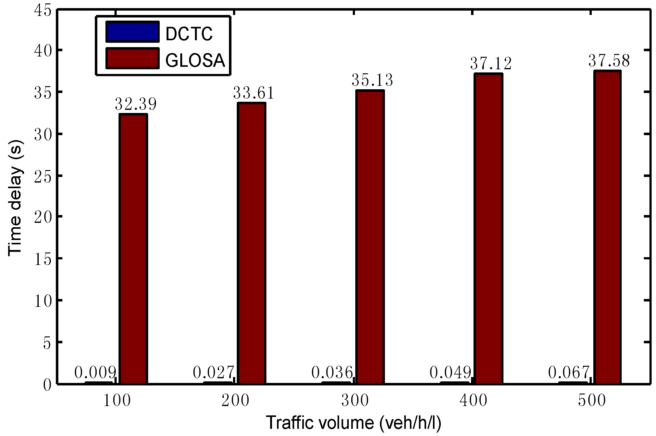
As a result, the DCTC can achieve a better performance than the GLOSA under the traffic volume from 100 (veh/h/l) to 500 (veh/h/l). As shown in Figure 8, the time delay in the DCTC is very low and much smaller than that in the GLOSA, which signifies that all the vehicles can finish their entire trip at a near maximal speed. In the DCTC, all the vehicles can pass the intersection without stopping, which can be reflected by the stop time in Figure 9. Furthermore, the DTCT can make the vehicles pass the intersection with a higher speed than the GLOSA in order to decrease the passing time, as shown in the Figure 10 and Figure 11. Therefore, the traffic efficiency is improved by releasing the intersection resource more quickly. The Figure 12 presents that the calculation time for the DCTC meets the real-time demand in different traffic volume.

5. Conclusions

This paper proposes a new cooperative and dynamic traffic control method for an isolated intersection with two lanes in each approach. With the V2I, the vehicles send their arrival time range to the intersection when they enter the communication zone. Then, in order to achieve the minimal time delay, the control center applies the ABC algorithm to optimize the passing sequence for the vehicles, where the compatible trajectories are combined dynamically. At last, after receiving the right-of-way, each vehicle plans its speed profile to meet the given sequence. The simulation results reveal that the proposed method can achieve lower time delay than other methods and make all the vehicles to finish their trip with a near maximal speed.

This study has potential limitations. For instance, the expected performance in this model is based on the assumption that the intersection only contains fully automatic vehicles with V2I. However, the future traffic stream should generally be mixed, with automatic vehicles, human drivers, and pedestrians, etc. In the future, this method can be extended to control an intersection network, and the priority for some special vehicles should be considered also. Moreover, the performance can be improved further by considering platooning during the passing sequence ordering processing in the case of multiple compatible and incompatible flow transfers [24,25].