Abstract
Hybrid powertrains that combine electric machines and internal-combustion engines offer substantial opportunities to increase the energy efficiency and minimize the exhaust emissions of vehicles and nonroad working machines. Due to the wide range of applications of such powertrains, simulation tools are used to evaluate and compare the energy efficiency of hybrid powertrains for application-specific working cycles in virtual environments. Therefore, the accurate modeling of the powertrain components of a hybrid system is important. This paper presents an agile calculation tool that can generate realistic fuel consumption data of a scalable diesel engine. This method utilizes a simple efficiency model of the combustion and crank train friction model to generate the fuel consumption map in the operating area of a typical diesel engine. The model parameters are calibrated to produce accurate fuel consumption data in the initial phase of system-level simulations. The proposed method is also validated by using three real engine datasets, and the comparison of results is presented.
1. Introduction
Increasingly tightening emission regulations and energy-efficiency demands are key drivers for the electrification of transportation and nonroad mobile machines. Hybrid electrical vehicles (HEV) provide the potential to reduce fuel consumption and consequently diminish CO emissions, since the workload of the machine is distributed between an internal-combustion engine (ICE) and electrical energy storage. HEV powertrain component designs can be studied through the simulation models of different vehicles and mobile machines. In energy-efficiency studies, accurate fuel consumption of the ICE in static loading condition is needed. Therefore, special attention should be paid to the efficiency and specific fuel consumption maps of diesel engine operation to aid in the estimation of fuel consumption in the system’s dynamic simulation [1].
The topology selection and dimensioning of hybrid powertrain components of offroad vehicles, such as agricultural tractors [2,3], different loaders [4], and forest machines [5], is a challenging task. The varying working operational profiles and demands of auxiliary devices of these vehicles make it difficult to evaluate the performance, fuel consumption, and feasibility of different control strategies of the vehicle under design. Simulators that can be used to evaluate and study these characteristics were introduced in previous studies [6]. Such simulation models are capable of simulating standard work cycles, testing powertrain components such as combustion engines, energy storage, and electrical drives, and changing the topology of the vehicle.
In typical combustion engine models, many parameters are determined on the basis of measurements. However, if efficiency maps and specific fuel consumption maps are available, a relatively simple simulation model can be created without relying on measurements. This stationary data can be combined with estimated or measured dynamics to limit the change in torque of the engine model. For initial design purposes, such a model, producing results that are sufficiently accurate to compare topologies, dimensioning selections, or control strategies, is adequate. However, the efficiency and specific consumption maps are often not available to designers. This sets a demand for a simulation method that can produce these maps on the basis of available engine manufacturer data.
General approaches of combustion engine gas exchange system simulation can be categorized as zero- (0D), one- (1D) and three-dimensional (3D) simulations. Contrarily, incylinder simulations are divided into thermodynamic (0D) and fluid dynamic approaches (1D or 3D) [7]. The 1D and 3D models are complex, require several engine-related parameters as input data, and are unsuitable for system-level studies as they are computationally expensive [8]. Simpler engine models were proposed for the development of system-level simulations and engine control units (ECUs). According to [9], such models are classified as 0D, mean-value (MVM), and transfer-function models, the simplest one being the transfer-function model, which can mainly describe the engine’s dynamic torque response. MVMs can be divided into crank-angle-based and non-crank-angle-based. The latter can be further divided into map- or thermodynamics-based approaches.
Map-based MVMs are accurate and fast, and are typically used for ECU development. An engine model with map-based description of the incylinder efficiency and engine crank-train friction was presented in [10]. The model was based on the Willans approximation for dynamic vehicle simulation, and it was developed for engine and exhaust gas aftertreatment simulations. A vehicle model consisting of several submodels, with look-up table-based incylinder combustion and fuel conversion efficiency was presented in [11]. The calibration of parameters using engine test bench data required in this model is a drawback. Typically, generating engine-efficiency maps requires large amounts of experimental data. However, these maps can also be created using complex and computationally expensive engine models, which can map the efficiencies and flow phenomena [12]. Engine fuel consumption and emissions were predicted in [13] using engine maps created by combining actual vehicle emission data with manufacturer-provided engine data.
Seiliger process description-based thermodynamic models were developed in several studies where the real changes of incylinder states were substituted by ideal processes such as constant volume, pressure, or temperature over the engine cycle [9,14,15]. Such simulations can predict pressure and temperature during the engine crank rotation cycle. They are faster compared to crank angle-based simulations, but they are not as accurate. A crank-angle-based model describing the fraction of burned mass of fuel during the combustion by a Wiebe exponent function was presented in [16]. The Wiebe function is an experimental curve used to predict the typical engine fuel energy released in the cylinder during the cycle [7]. If the Wiebe function parameters are correctly determined, this approach can be more accurate than Seiliger-based calculations. An excavator model was developed in [17] for duty-cycle simulations of working machines, where the engine was modeled with 0D quasisteady-flow modeling approach, and calibrated to the real natural aspirated diesel engine at full-load curve. In this approach, the engine’s partial load performance can be predicted using the manufacturer-provided full-load torque of the engine.
A thermodynamic incylinder model was developed using the Wiebe function for energy conversion and Arrhenius correlation for the fuel ignition delay in [18], where the cylinder temperature was depicted in one temperature area to improve the prediction capability. This model was extended to predict emissions by using Zeldovich’s formula in [19] and modified from a single zone incylinder model to a two-zone one in [20]. An engine model for passenger car driving cycle simulations was developed in [21], where the intake air pressure and instant volumetric efficiency were taken from an experimental look-up table, and the fuel injection and heat release rate were modeled using complex nonlinear correlation formulas. Such models are too complex for concept-phase study and require a large amount of experimental data from existing engines. Several papers have presented mathematical methods to improve engine models using neural networks and different kinds of deterministic or stochastic models. These methods achieve fast and more accurate simulation results by improving the fitting of the model parameters. Such methods can also be used to develop black-box models that do not include any physical description. However, such models have limited prediction capability and require a large amount of experimental data [22,23,24].
The reviewed literature encompasses the varied approaches to modeling engine simulation tools. The reviewed methods reflect a prime focus on the development of highly accurate complex engine models. The intensive computational demands and the wide array of required experimental data of specific engines make these models unsuitable for initial design purposes. To conduct energy-efficiency studies on hybrid powertrain concepts, we need generic engine models that enable system-level studies with sufficient accuracy. General-purpose scalable engine models suitable for such purposes are not presented in the reviewed literature.
This study presents an agile calculation tool that can generate realistic diesel engine data for the purpose of developing powertrains for working machines. This method utilizes a simple engine-efficiency model and crank train friction model to generate a realistic engine fuel consumption map in a wide operating area of the engine. The maximal torque curve and its specific fuel consumption as a function of speed are needed as input data. Additionally, basic engine data, such as cylinder dimensions and number, are needed. These data are typically published by the engine manufacturer. The proposed model can be calibrated to produce accurate prediction of the by tuning certain calculation parameters. Consequently, partial load can also be calculated by using the calibrated parameters. The presented calculation tool with calibrated parameters produces an accurate and realistic behavior of fuel consumption and shaft power outputs without using large amounts of experimental data or complex physics-based engine models. The presented method is validated by calculating three different sets of measured engine fuel consumption data. The comparison between calibrated and uncalibrated calculation results is also presented.
2. Engine Power and Specific Fuel Consumption
Engine manufacturers typically provide basic construction data, e.g., number of cylinders, cylinder bore diameter, and stroke as the technical data of the engine. The rated shaft power and maximal torque are normally presented as the performance data of the engine. However, the fuel consumption or efficiency of the engine, especially in partial loads, is not published. Fuel consumption in a wide operation range is needed in different types of hybrid powertrain simulations. The method presented in this study utilizes the full-load torque curve and specific fuel consumption curve , which is published by an engine manufacturer as a function of engine speed in full load, as presented in Figure 1.
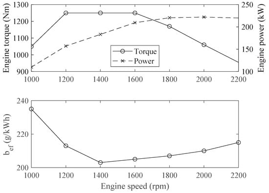
Figure 1.
Example of a typical engine’s full-load power, torque, and specific fuel consumption curves according to engine manufacturer’s brochure [25].
According to [7], the specific fuel consumption () of the engine typically reaches its minimal value when engine speed and load are close to the maximal torque operation point. increases in low loads; thus, the relative part of crank train friction is relatively higher, and losses are increased. At high speed, friction is also increased and decreased; otherwise, combustion efficiency decreases when speed is high. Accordingly, the shapes of maps have similarities in different engines.
The proposed calculation method is based on the model presented in [26]. The original model is a mean-value engine model, and it was initially developed for the control system purposes and software or hardware in loop (SiL/HiL) simulations. The original method includes several submodels for engine subsystems, and some of these are suitable for spark-ignited engines, diesel engines, or both. The original submodels on which this study is based are presented in Table 1. Of those, the ETH friction model for crank train friction, engine speed-related indicated efficiency, and injection timing effect to indicated efficiency, was implemented. These models were also simplified due to limited initial specification of the engine. In this study, the diesel engine parameters presented in [26] were used as the initial parameters of this study, and are shown in Table 5. By this method, the shape of specific fuel consumption map of the diesel engine can be predicted from the full-load data provided by engine manufacturers.This manufacturer’s data should include at minimum 3–5 individual measured data points, which present the engine’s full-load torque and specific fuel consumption in these points, as presented in Figure 1. To improve the original model and increase the prediction accuracy, three input parameters of the model are used to calibrate the calculation.

Table 1.
Original structure of calculation method and submodels in Section 2.5 (Mechanical systems) of [26]. Bolded submodels are used in this study.
The proposed calculation method includes four steps as shown in Figure 2. In the first step, the full torque curve data of the suitable engine were chosen from the literature or the engine manufacturer’s catalog. In the second step, the specific fuel consumption values were calculated by using basic parameters of the chosen engine in the model (Equation (8)). In the third step, these values were compared to the real engine. If the relative differences in the values were above 3%, the model parameters need to be calibrated. After the calculated values are brought within the tolerance limits, the specific fuel consumption at partial load can be calculated using the calibrated model parameters (Equation (8)).
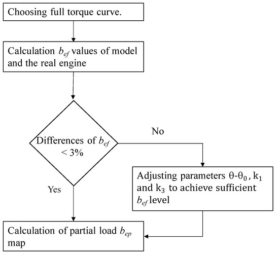
Figure 2.
Calculation procedure structure and parameter calibration.
The indicated efficiency of the engine applies to the conversion of fuel energy into mechanical work up to the piston top. In this model, the submodel named engine speed describes the indicated efficiency of the engine as a function of engine speed (Table 2). To implement the values in Table 2 in the calculation program, the data were fitted to the second-order polynomial curve as a function of engine speed. The fitted polynomial parameters are shown in Equation (1).
where is the indicated efficiency, n is the engine speed, and is the injection timing effect.

Table 2.
Typical indicated efficiency values of diesel engines as a function of speed [26].
The fuel injection timing of the engine strongly affects the indicated efficiency. Although the real engine injection timing is not known and it cannot be implemented in the model, this parameter is needed for the calibration purpose of the model. The effect of the fuel injection timing can be considered according to [26], as follows.
where is the timing coefficient, is the injection timing angle, and is the injection timing that produces maximal brake torque.
The crank train friction model is needed to calculate the net power output of the engine from the indicated power. For this purpose, the ETH friction model was implemented in this method. The ETH friction model was originally presented in [27] and used in [26]. The original ETH friction model includes coefficients for the maximal boost ratio and for engine coolant temperature, which were not implemented in this study. The crank train friction can be set to a sufficient level during the calibration procedure without using these coefficients. The crank train friction of the engine is a function of the crank train dimensions, speed, and engine temperature. It can be presented as a friction mean effective pressure (), as follows.
where S is the stroke of the engine, is the angular velocity of the engine, B is the cylinder bore of the engine, is engine temperature behavior coefficient, and are the coefficients of the crank train geometry of the engine.
Figure 3 shows the calculation program structure and the input parameters needed to calculate the specific fuel consumption at each engine operation point. Using the friction mean effective pressure () calculated from Equation (3), the friction power of the engine () can be expressed as follows:
where is the engine cylinder displacement, n is the engine speed, and is the number of revolutions per power stroke of the engine.
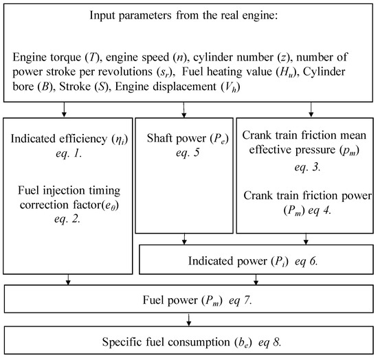
Figure 3.
Calculation program structure and calculation order.
The engine output power () can be calculated from the torque and speed using Equation (5).
where T is the engine torque, and n is the engine speed.
The engine indicated power () can be calculated using Equation (6).
where is the engine shaft power, and is the crank train friction power of the engine.
The fuel input energy in a specific operation point can be determined by calculating the power of fuel energy flow :
where is the indicated power of the engine, and is the indicated efficiency of the engine.
In the final step, the specific fuel consumption () can be calculated as
where is the fuel power, is the shaft power, and is the fuel heating value.
The presented method calculates the specific fuel consumption at a given torque and speed point. The real engine fuel consumption varies widely depending on the different technical solutions and functional parameters of the engine. Some model parameters are used for calibration purposes, as presented in Figure 2. The full-load curve of the engine is the reference level, where specific fuel consumption level is calibrated using certain submodel parameters. Official standards of the engine’s power rating and exhaust emissions set the experimental measuring accuracy of the engine power output and fuel mass flow typically in the range of ±2–3% [28,29]. Thus, the specific fuel consumption calculation tolerances are in the range of 3–5%. An accuracy level of 3% relative differences is the acceptable tolerance of the calibrated values of in this study.
3. Calculation Method Comparison, Calibration, and Validation Using Real Engine Results
To validate the accuracy of the calculation method, results obtained from the model and measurements from three different real engines were compared. The first engine was an AGCO Power 49. Engine performance and specific fuel consumption and were measured in the engine and powertrain laboratory of Turku University of Applied Sciences. The engine performance characteristics over a wide speed and torque range were measured for exhaust emission research. However, the exhaust emission results were not used in this study. The research test runs were produced in a steady-state mode; thus, the engine speed and torque output were constant, while the fuel consumption and produced power were measured over 1 min of average results. This method produces an accurate fuel consumption map at a steady engine load condition. The laboratory instruments used in the measurements are presented in Table 3, and the test bench setup in Figure 4.

Table 3.
Experimental setup and instruments.
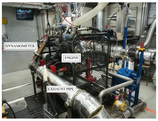
Figure 4.
Experimental setup of AGCO Power 49 engine.
Two other engines’ measurement datasets were presented in the literature. The engine manufacturer, Scania, Södertälje, Sweden, published some of their engine’s fuel consumption in partial load conditions [30]. This Scania engine was chosen as the second engine. The data of the third chosen engine were presented in [31]. The specific fuel consumption was presented as a third-degree polynomial regression model for the Iveco 8460 engine. This regression was based on the experimental measurements. All these engines were turbocharged, 4-stroke diesel engines and equipped with a charge air cooling system. The main features of the compared engines are presented in Table 4.

Table 4.
Main specification of compared engines.
Engines were modelled, and calculation results for the results were compared to the real engine results. For the initial parameter values, which are presented in Table 5, the values of [26] were used. When the calculated differed more than 3% from the real engine values, the calculation parameters were manually calibrated to reach the sufficient correspondence, as indicated by the procedure presented in Figure 2. Partial loads were calculated using the calibrated model parameters. The values of the original parameters and calibrated parameters of each engine are presented in Table 5.

Table 5.
Basic and calibrated parameters of each engine model.
When the AGCO Power 49 engine cylinder geometry (Table 4) and calculation parameters (Table 5) were implemented in the calculation model, differences were between −1.6% and 0.8% at the full-load points. The accuracy of the results was within the decided limits; hence, no parameter calibration was performed. At the next phase, partial load was calculated. In the 50% power curve, the calculated was 5–6% higher than that of the real engine, and in 25% load calculation, it was 6–10% higher than that of the real engine. Figure 5 shows the simulated map of the AGCO engine in load range 25–100%, and the percentage differences between the calculated and real values of .
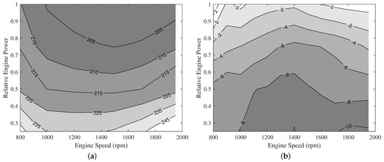
Figure 5.
Results obtained from AGCO Power 49 engine model. (a) Specific fuel consumption (g/kWh) map calculated by the model. (b) Percentage differences between calculated and measured values of .
Next, the calculated and measured results for the Scania engine were compared. The Scania engine’s cylinder geometry, model parameters, and initial values were implemented in the model. Differences between measured and calculated values of at full load are presented in Figure 6. At the speed of 1200 rpm, the calculated value was 1.7% higher than the measured value. However, around the speed of 1550 rpm, the measured value started to surpass the calculated value. Lastly, at the speed of 2100 rpm, the measured value exceeded the calculated value by 7.1%.
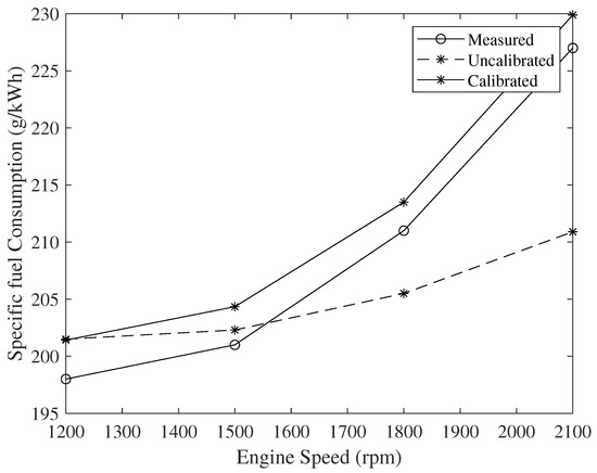
Figure 6.
Calculated compared to Scania DC 09 engine full-load curve.
Since the differences between the measured and calculated results at high speeds exceeded the threshold of 3%, the parameters were calibrated using a trial-and-error method. The fuel injection timing effect parameters were calibrated, such that they could be expressed as a function of engine speed n, as described in Table 5. In addition, parameters and were manually modified from 1.44 to 1.2 and 1.1 × 10 to 1.6 × 10 s/m, respectively. Using this manual trial-and-error-based calibration, the difference between the measured and calculated results at full load was brought down to a range of 1.2–1.7% for the Scania engine, as shown in Figure 6.
Figure 7 shows the calculated and calibrated map of the Scania engine model in the load range of 50–100%, and the percentage difference between the calculated and real values of . Calculation errors were high in the lower power ranges. At 75% load, differences were between −2.5% and 2.1%, and at 50% load, differences were between −9.6% and 1.3%. When focusing on the 50% load region, between 1800 and 2100 rpm, measured value of noticeably increased, and the model could not predict such phenomena. However, the differences between the calculated and real engine values were less than 10% over the studied operation range of the Scania engine.
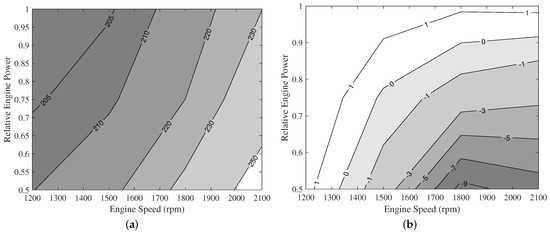
Figure 7.
Results obtained from SCANIA DC 09 engine model. (a) Specific fuel consumption (g/kWh) map calculated by model. (b) Percentage differences between calculated and measured values of .
Figure 8 shows the calibrated and calculated map in the load range of 25–100% for the third studied engine, Iveco 8460. Reference values were obtained from the three-dimensional regression of in [31]. The regression map was based on the experimental measurements. Calculations with the initial parameters produced a significantly lower value than that of the real engine, due to which calibration was performed. Therefore, calculation parameter was increased from 1.1 × 10 to 1.6 × 10 Pa. The injection timing effect was modified to change as a term of engine speed as presented in Table 5. With these changes, differences between the values of the regression and calculation results were reduced to 1% at full load. Figure 8 also shows the percentage difference between the calculated and regression values of for this engine in the load range of 25–100%. The differences were highest at the speed of 2200 rpm, under 50% load with a value of −5.3%. In other high-speed areas, differences were between −2.8% and +0.9%.
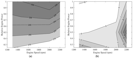
Figure 8.
Results obtained from Iveco 8460 engine model. (a) Specific fuel consumption (g/kWh) map calculated by model. (b) Percentage differences between calculated and measured values of .
Using the presented method, different kinds of engine models can be created, and fuel consumption in the operation area can be calculated with sufficient accuracy for energy-efficiency studies when the full torque curve and its fuel consumption are available. This method is suitable and can be scaled to four stroke diesel engines that are turbocharged and charge-cooled in the power range of approx. 50–500 kW. Engines below 50 kW typically use a simpler fuel injection system, and there are naturally aspirated engines widely used in this power range; thus, the accuracy of this method can be insufficient. Engines above 500 kW typically have a narrow speed range, and the shape of the fuel consumption maps can be of different types. However, the suitable power range covers a wide spectrum of engines for hybrid-powertrain studies. This method is utilized in the study [32], to produce maps of engines in the power range 64–202 kW for the hybrid simulation of mobile machines.
The AGCO and Scania engines are modern and use selective catalytic reduction (SCR) technology for the abatement of NOx emissions. Typically, NOx levels in engine-out can be higher than those in engines without SCR. Thus, fuel consumption can be optimized to a lower level for engines without SCR. The Iveco engine was approximately 10 to 15 years older than the AGCO Power and Scania engines, and not equipped with SCR technology. That is a possible reason behind the higher level of Iveco. The Scania engine also uses exhaust gas recirculation (EGR) for emission reduction. This may have increased the Scania engine’s fuel consumption in high engine speeds when compared to the AGCO Power engine. However, the operation range of the Scania engine was also in a higher speed range than that of the AGCO Power engine.
4. Conclusions
In this paper, a simple calculation method for the specific fuel consumption map of a scalable combustion engine was presented. Results of the calculation method were fitted to the measured data of three different actual engines at full load, which is typically provided by the engine manufacturer. Then, the partial-load fuel consumption was calculated using the calculation method, and results were compared to the real engine curves. Calculation parameters were calibrated by trial and error to produce higher-accuracy results whenever required. For future improvements of this model, a more sophisticated calibration algorithm can be utilized. Differences between the calculated and actual values were below 10% in the engine load range of 25–100% for the studied engines after calibration. The presented method can thus predict the engine power generation capability with sufficient accuracy for the purposes of a concept study of hybrid powertrain simulations. In the future, engine air flow and thermal balance or exhaust temperature estimation methods can be studied. The turbocharged engine dynamic behavior is also a subject of interest.
Author Contributions
Conceptualization, M.L.; methodology, M.L.; software, M.L.; validation, M.L.; formal analysis, M.L.; investigation, M.L.; resources, T.L., J.S.; data curation, M.L.; writing—original draft preparation, M.L., A.T., T.L.; writing—review and editing, G.G., A.T., S.J.; visualization, M.L., S.J.; supervision, T.L., J.S.; project administration, T.L., J.S.; funding acquisition, T.L., J.S., M.L. All authors have read and agreed to the published version of the manuscript.
Funding
The research was funded by Business Finland (Project No. 3007/31/2019 and 5376/31/2018).
Institutional Review Board Statement
Not applicaple.
Informed Consent Statement
Not applicaple.
Data Availability Statement
Not applicable.
Acknowledgments
The authors thanks the engine and powertrain laboratory staff of Turku University of Applied Sciences for the experimental research, and AGCO Power Inc. for the collaboration concerning the experimental engine data.
Conflicts of Interest
The authors declare no conflict of interest.
References
- Sabri, M.; Danapalasingam, K.A.; Rahmat, M.F. A review on hybrid electric vehicles architecture and energy management strategies. Renew. Sustain. Energy Rev. 2016, 53, 1433–1442. [Google Scholar] [CrossRef]
- Jaiswal, S.; Åman, R.; Sopanen, J.; Mikkola, A. Real-time multibody model-based heads-up display unit of a tractor. IEEE Access 2021, 9, 57645–57657. [Google Scholar] [CrossRef]
- Jaiswal, S.; Korkealaakso, P.; Åman, R.; Sopanen, J.; Mikkola, A. Deformable terrain model for the real-Time multibody simulation of a tractor with a hydraulically driven front-loader. IEEE Access 2019, 7, 172694–172708. [Google Scholar] [CrossRef]
- Jaiswal, S.; Islam, M.; Hannola, L.; Sopanen, J.; Mikkola, A. Gamification procedure based on real-Time multibody simulation. Int. Rev. Model. Simul. 2018, 11, 259–266. [Google Scholar]
- Baharudin, M.E.; Rouvinen, A.; Korkealaakso, P.; Mikkola, A. Real-time multibody application for tree harvester truck simulator. Proc. Inst. Mech. Eng. Part K J. Multibody Dyn. 2014, 228, 182–198. [Google Scholar] [CrossRef]
- Nokka, J. Energy Efficiency Analyses of Hybrid Non-Road Mobile Machinery by Real-Time Virtual Prototyping. Ph.D. Thesis, Lappeenranta University of Technology, Lappeenranta, Finland, 2018. [Google Scholar]
- Heywood, J.B. Internal Combustion Engine Fundamentals; McGraw-Hill Education: New York, NY, USA, 2018. [Google Scholar]
- Lee, S.Y.; Andert, J.; Pischinger, S.; Ehrly, M.; Schaub, J.; Koetter, M.; Ayhan, A.S. Scalable Mean Value Modeling for Real-Time Engine Simulations with Improved Consistency and Adaptability; Technical report, SAE Technical Paper; SAE International: Warrendale, PA, USA, 2019. [Google Scholar]
- Theotokatos, G. On the cycle mean value modelling of a large two-stroke marine diesel engine. Proc. Inst. Mech. Eng. Part M J. Eng. Marit. Environ. 2010, 224, 193–205. [Google Scholar] [CrossRef]
- Dahl, J.; Andersson, D. Engine air path management and exhaust condition modeling in Dymola. Int. J. Engine Res. 2014, 15, 993–1008. [Google Scholar] [CrossRef]
- Eriksson, L.; Lindell, T.; Leufven, O.; Thomasson, A. Scalable component-based modeling for optimizing engines with supercharging, E-boost and turbocompound concepts. SAE Int. J. Engines 2012, 5, 579–595. [Google Scholar] [CrossRef]
- Klein, S.; Savelsberg, R.; Xia, F.; Guse, D.; Andert, J.; Blochwitz, T.; Bellanger, C.; Walter, S.; Beringer, S.; Jochheim, J.; et al. Engine in the loop: Closed loop test bench control with real-time simulation. SAE Int. J. Commer. Veh. 2017, 10, 95–105. [Google Scholar] [CrossRef]
- Rosero, F.; Fonseca, N.; López, J.M.; Casanova, J. Real-world fuel efficiency and emissions from an urban diesel bus engine under transient operating conditions. Appl. Energy 2020, 261, 114442. [Google Scholar] [CrossRef]
- Sui, C.; Song, E.; Stapersma, D.; Ding, Y. Mean value modelling of diesel engine combustion based on parameterized finite stage cylinder process. Ocean Eng. 2017, 136, 218–232. [Google Scholar] [CrossRef] [Green Version]
- Murphy, A.; Norman, A.; Pazouki, K.; Trodden, D. Thermodynamic simulation for the investigation of marine Diesel engines. Ocean Eng. 2015, 102, 117–128. [Google Scholar] [CrossRef] [Green Version]
- Giglio, V.; di Gaeta, A. Novel regression models for Wiebe parameters aimed at 0D combustion simulation in spark ignition engines. Energy 2020, 210, 118442. [Google Scholar] [CrossRef]
- Casoli, P.; Gambarotta, A.; Pompini, N.; Riccò, L. Coupling excavator hydraulic system and internal combustion engine models for the real-time simulation. Control Eng. Pract. 2015, 41, 26–37. [Google Scholar] [CrossRef]
- Maroteaux, F.; Saad, C. Diesel engine combustion modeling for hardware in the loop applications: Effects of ignition delay time model. Energy 2013, 57, 641–652. [Google Scholar] [CrossRef]
- Maroteaux, F.; Saad, C.; Aubertin, F. Development and validation of double and single Wiebe function for multi-injection mode Diesel engine combustion modelling for hardware-in-the-loop applications. Energy Convers. Manag. 2015, 105, 630–641. [Google Scholar] [CrossRef]
- Maroteaux, F.; Saad, C. Combined mean value engine model and crank angle resolved in-cylinder modeling with NOx emissions model for real-time Diesel engine simulations at high engine speed. Energy 2015, 88, 515–527. [Google Scholar] [CrossRef]
- Finesso, R.; Spessa, E.; Yang, Y. Development and validation of a real-Time model for the simulation of the heat release rate, in-Cylinder Pressure, and pollutant emissions in diesel engines. SAE Int. J. Engines 2016, 9, 322–341. [Google Scholar] [CrossRef]
- Sujesh, G.; Ramesh, S. Modeling and control of diesel engines: A systematic review. Alex. Eng. J. 2018, 57, 4033–4048. [Google Scholar] [CrossRef]
- Vong, C.M.; Wong, P.K.; Li, Y.P. Prediction of automotive engine power and torque using least squares support vector machines and Bayesian inference. Eng. Appl. Artif. Intell. 2006, 19, 277–287. [Google Scholar] [CrossRef]
- Hao, D.; Zhao, C.; Li, Y.H.G.; Zeng, W.; Li, H. Dynamic indicated torque estimation for turbocharged diesel engines based on back propagation neural network. IFAC-PapersOnLine 2018, 51, 720–725. [Google Scholar] [CrossRef]
- IvecoMotors. Iveco Cursor 78ENT Engine Broschyre. Available online: https://www.tapimer.fi/wp-content/uploads/2016/09/C78ENT-220kW.pdf (accessed on 6 April 2021).
- Guzzella, L.; Onder, C. Introduction to Modeling and Control of Internal Combustion Engine Systems; Springer Science and Business Media: Berlin/Heidelberg, Germany, 2009. [Google Scholar]
- Stöckli, M. Reibleistung von 4-Takt Verbrennungsmotoren; Technical Report, Internal Report of the Laboratory of Internal Combustion Engines; ETH Zürich: Zürich, Switzerland, 1989. [Google Scholar]
- Directive 1999/96/EC. 1999. Available online: https://eur-lex.europa.eu/legal-content/EN/TXT/PDF/?uri=CELEX:31999L0096&from=EN (accessed on 23 August 2021).
- ISO 3046-1:2002. Reciprocating Internal Combustion Engines—Performance—Part 1: Declarations of Power, Fuel and Lubricating Oil Consumptions, and Test Methods—Additional Requirements for Engines for General Use. 2002. Available online: https://www.iso.org/standard/28330.html (accessed on 15 August 2021).
- Scania. Scania DC09 084A 202kW Engine Broschyre. Available online: https://www.scania.com/content/dam/scanianoe/market/master/products-and-services/engines/pdf/specs/industry/DC984A_202kW_SCR.pdf (accessed on 6 April 2021).
- Corredor, L.; Escobar, A.; Portnoy, I.; Vélez, E. Prediction of specific fuel consumption in turbocharged diesel engines under partial load performance. Renew. Energy Power Qual. J. 2012, 1, 1558–1562. [Google Scholar] [CrossRef]
- Tupitsina, A.; Montonen, J.; Alho, J.; Immonen, P.; Lauren, M.; Lindh, P.; Lindh, T. Simulation tool for dimensioning power train of hybrid working machine. Model. Identif. Control 2021, 42, 143–158. [Google Scholar] [CrossRef]
Publisher’s Note: MDPI stays neutral with regard to jurisdictional claims in published maps and institutional affiliations. |
© 2021 by the authors. Licensee MDPI, Basel, Switzerland. This article is an open access article distributed under the terms and conditions of the Creative Commons Attribution (CC BY) license (https://creativecommons.org/licenses/by/4.0/).