Article

Distribution Tableaux, Distribution Models

by
J.-Martín Castro-Manzano
Faculty of Philosophy, UPAEP University, Puebla 72410, Mexico
Axioms 2020, 9(2), 41; https://doi.org/10.3390/axioms9020041
Submission received: 3 December 2019 / Revised: 24 March 2020 / Accepted: 26 March 2020 / Published: 17 April 2020
(This article belongs to the Special Issue Deductive Systems in Traditional and Modern Logic)

Abstract

:
The concept of distribution is a concept within traditional logic that has been fundamental for the syntactic development of Sommers and Englebretsen’s term functor logic, a logic that recovers the term syntax of traditional logic. The issue here, however, is that the semantic counterpart of distribution for this logic is still in the making. Consequently, given this disparity between syntax and semantics, in this contribution we adapt some ideas of term functor logic tableaux to develop models of distribution, thus providing some alternative formal semantics to help close this breach.

1. Introduction

The concept of distribution is a concept within traditional logic that is applied when a term appears under the scope of a universal quantifier. Thus, for example, in the proposition “All men are mortal” we say the term “men” is distributed whereas the term “mortal” is not. In spite of its simplicity, the importance of this concept is far from being overstated, given that it allows us to define rules essential to syllogistic, a term logic at the core of traditional logic; however, specially since the objections raised by Geach [1], distribution—as traditional logic—is seemingly out of favor.
Nevertheless, distribution serves a logical purpose (cf. [2,3,4,5]) that has been fundamental for the syntactic development of Sommers and Englebretsen’s term functor logic, a logic that recovers the term syntax of traditional logic [4,6,7]. The issue here, however, is that the formal semantics counterpart of distribution for this logic is still in the making. Of course, it goes without saying that Sommers and Englebretsen have already provided semantic standards for their logic, but such semantics are philosophical rather than formal, so to speak (cf. [6,8]). Consequently, given this disparity between syntax and semantics, in this contribution we adapt some ideas of term functor logic tableaux [9] to develop models of distribution, thus providing some alternative formal semantics to help close this breach.
In order to reach this goal we proceed in the following way. First we expound some preliminaries about syllogistic, distribution, and term functor logic and its tableaux; then we develop our main contribution by exploring some links between the rules of term functor logic and the concept of the model.

2. Preliminaries

2.1. Syllogistic

Syllogistic is a logic term at the core of traditional logic that deals with inference between categorical propositions. A categorical proposition is a proposition composed by two terms, a quantity, and a quality. The subject and the predicate of a proposition are called terms: the term-schema S denotes the subject term of the proposition and the term-schema P denotes the predicate. The quantity may be either universal (All) or particular (Some), and the quality may be either affirmative (is) or negative (is not). These categorical propositions have a type denoted by a label (either a (universal affirmative, SaP ), e (universal negative, SeP ), i (particular affirmative, SiP ), or o (particular negative, SoP )) that allows us to determine a mood, that is, a sequence of three categorical propositions ordered in such a way that the first two propositions are premises (major and minor) and the last one is a conclusion. A categorical syllogism, then, is a mood with three terms one of which appears in both premises but not in the conclusion. This particular term, usually denoted with the term-schema M , works as a link between the remaining terms and is known as the middle term. According to the position of this middle term, four figures can be set up in order to encode the valid syllogistic moods (Table 1) (for sake of brevity, but without loss of generality, we omit the syllogisms that require existential import).

2.2. Distribution

Now, in order to determine the validity of the previous moods we can invoke the concept of distribution since, as we mentioned before, it allows us to define rules instrumental for showing the validity of such inferences. These rules state (i) that a syllogistic inference is valid if and only if for every term A , if A is distributed in the conclusion, then A is distributed in the premises as well; and (ii) that a syllogistic inference is valid if and only the middle term M is distributed once in the premises. Thus, for instance, the following inference (Table 2) is valid since the term “dogs” is distributed in the conclusion and in the minor premise; and the middle term, “mammals,” is distributed once in the premises (at the major premise).
Previously we claimed that the concept of distribution is applied when a term appears under the scope of a universal quantifier, but the very concept of distribution is far from being clear, given that there are several accounts of it. For example, according to some medieval theories of supposition a term is said to be distributed in a proposition when such a term refers to all that it means, as when a term is under the scope of a universal quantifier. In this sense we can understand, for instance, the notion of Peter of Spain [10], who talks of distribution as multiplicatio termini communis per signum universale facta (i.e., [distribution is] the multiplication of the common term made by a universal sign (translation and emphasis are ours)) or the notion advanced by the Port-Royal tradition [11] that claims that to say that a term is distributed in a proposition is to say that such a term doit être pris universellement (i.e., must be taken universally (translation and emphasis are ours)).
Nevertheless, the notion of distribution developed by Keynes [12]—and well defended by Sommers [3] and Wilson [5], in our opinion—is probably worth mentioning, since this is the one that Geach [1] discusses. Keynes’ idea is that a term is said to be distributed when reference is made to all the items denoted by it; and it is said to be undistributed when they are only referred to partially. More formally, and following [3], we assume that a term A is distributed in a proposition p in the next sense:
  • A is distributed in p if and only if p entails a proposition of the form “every A is
  • A is not distributed in p if and only if A is distributed in the contradictory of p.
Hence for syllogistic we say that, given its quantity and its quality, a categorical proposition distributes its terms if and only if they have a universal quantity or a negative quality: this will be formalized in the next section with the help of term functor logic.

2.3. Term Functor Logic
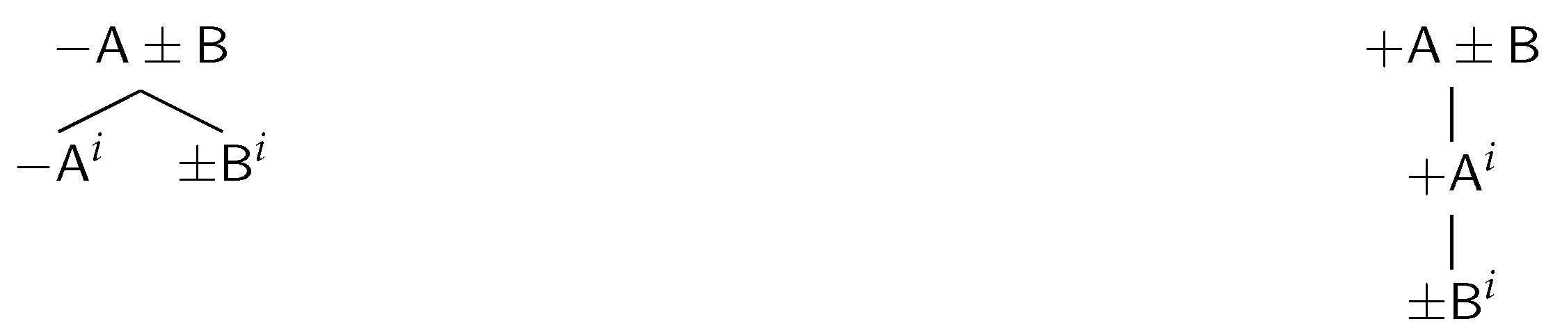
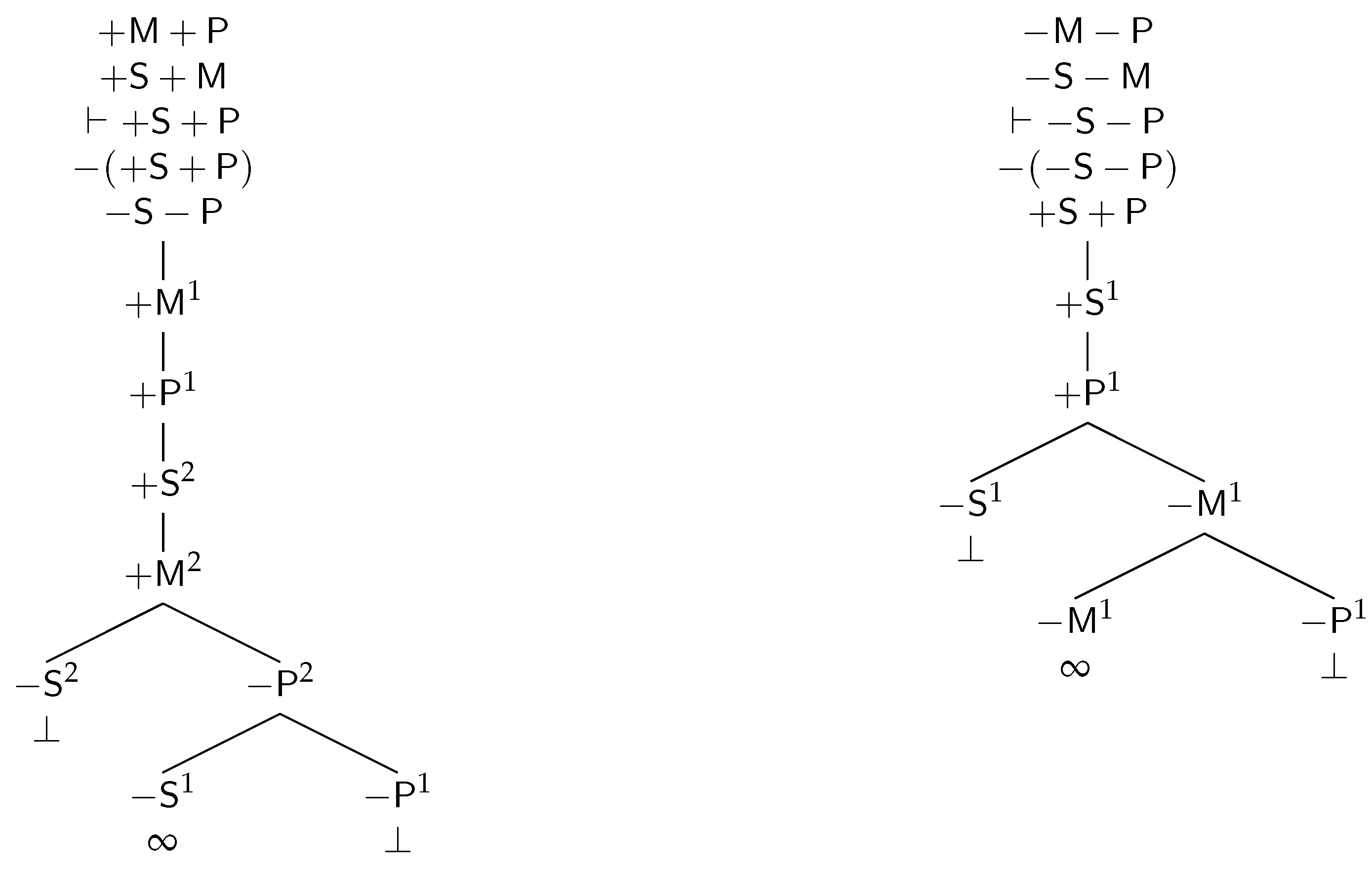
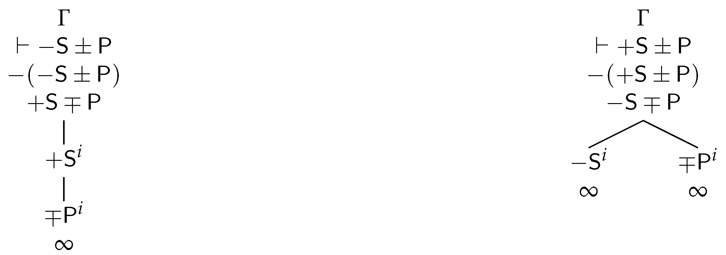
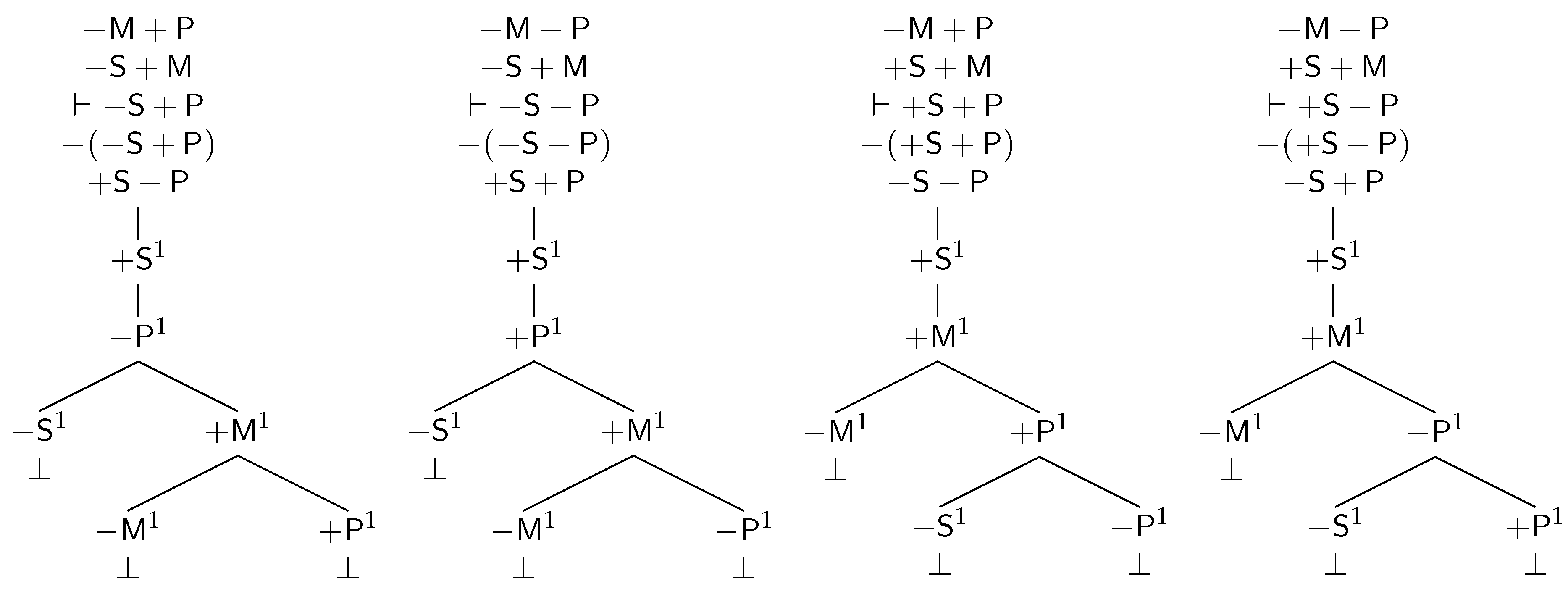
Term Functor Logic (TFL, for short) is a plus-minus algebra [4,6,7,13,14,15] that employs terms rather than first order language elements such as individual variables or quantifiers (cf. [4,16,17,18,19]). According to this algebra—or “logibra”, as Sommers dubbed it—, the four categorical propositions can be represented by the following syntax [6], where “−” indicates that a term is distributed, and “+” that a term is not distributed:
  • SaP : = S + P = S ( P ) = ( P ) S = ( P ) ( + S )
  • SeP : = S P = S ( + P ) = P S = P ( + S )
  • SiP : = + S + P = + S ( P ) = + P + S = + P ( S )
  • SoP : = + S P = + S ( + P ) = + ( P ) + S = + ( P ) ( S )
Given this representation, this plus-minus algebra provides a simple rule for syllogistic inference: a conclusion follows validly from a set of premises if and only if (i) the sum of the premises is algebraically equal to the conclusion and (ii) the number of conclusions with particular quantity (viz., zero or one) is the same as the number of premises with particular quantity ([6] p. 167). This rule is an algebraic rendition of the dictum de omni et nullo (this is the principle that states that everything that is affirmed (or denied) of a whole can be affirmed (or denied) of a part (cf. [4,6,7,14,20]))—hence its name, DON—and can be formally deployed as follows:
Γ ϕ i f f { ( i ) a l g ( Γ ) = a l g ( ϕ ) , a n d ( i i ) | p a r t i c u l a r s ( Γ ) | = | p a r t i c u l a r s ( ϕ ) |
where Γ stands for a (possibly empty) set of premises; ϕ stands for a conclusion; a l g for an algebraic sum; and | p a r t i c u l a r s | for a function that returns the number of particular propositions in a set of terms.
Thus, for instance, if we consider a valid syllogism, say the mood aaa from the first figure (i.e., aaa -1), we can see how the application of DON produces the right conclusion (Table 3).
Indeed, in the previous example we can clearly see how the rule works: (i) if we add up the premises we obtain the algebraic expression ( M + A ) + ( D + M ) = M + A D + M = D + A , so that the sum of the premises is algebraically equal to the conclusion and the conclusion is D + A , rather than + A D , because (ii) the number of conclusions with particular quantity (zero in this case) is the same as the number of premises with particular quantity (zero in this case). Additionally, we must mention that this algebraic approach is not only capable of representing syllogistic, since it can also represent relational, singular, and compound propositions with ease and clarity while preserving its main idea, namely, that inference is a logical procedure between terms [14].

2.4. TFL Tableaux

Now, since alternative proof methods for TFL are still in the making, [9] has developed tableaux for it. So, following [21,22] we say a tableau is an acyclic connected graph determined by nodes and vertices, or more precisely, a labeled directed rooted tree. The node at the top is called the root. The nodes at the bottom are called tips. Any path from the root down a series of vertices is a branch. To test an inference for validity we construct a tableau which begins with a single branch at whose nodes occur the premises and the rejection of the conclusion: this is the initial list. We then apply the rules that allow us to extend the initial list (Scheme 1).
In Scheme 1, from left to right, the first rule is the rule for a ( e ) propositions, and the second rule is the rule for i ( o ) propositions. Notice that, after applying a rule, we introduce some index i { 1 , 2 , 3 , } . For propositions a and e , the index may be any number; for propositions i and o , the index has to be a new number if they do not already have an index. In addition, following TFL tenets, we assume the followings rules of rejection: ( ± A ) = A , ( ± A ± B ) = A B , and ( A A ) = + ( A ) + ( A ) .
As usual, a tableau is complete if and only if every rule that can be applied has been applied. A branch is closed if and only if there are terms of the form ± A i and A i on two of its nodes; otherwise it is open. A closed branch is indicated by writing a ⊥ at the end of it; an open branch is indicated by writing ∞. A tableau is closed if and only if every branch is closed; otherwise it is open. So, again as usual, A is a logical consequence of the set of terms Γ (i.e., Γ A ) if and only if there is a complete closed tableau whose initial list includes the terms of Γ and the rejection of A (i.e., Γ { A } ). Accordingly, up next we provide proofs of the valid syllogistic moods of the first figure (Scheme 2).
To describe the process we follow to unfold each tableaux consider the first one. The first three lines are the premises (major and minor) and the conclusion, and the fourth line is the rejection of the conclusion: all these lines but the conclusion define the initial list. Then the fifth line is the result of applying a rule of rejection to the conclusion. Then the next couple of lines is the result of applying the rule for an i proposition to the fifth line, picking index 1. Then the first split results from applying the rule for an a proposition to the second line (i.e., the minor premise), also picking index 1, since we want the indexes to unify. This split produces two branches, one of which (the leftmost) includes terms + S 1 and S 1 on two of its nodes, and hence is closed; the remaining branch is not closed yet, so we continue with the same process: we split the last available premise (the major one) to obtain, again, a couple of branches, one of which (the leftmost) includes terms M 1 and + M 1 on two of its nodes, and hence is closed; and the other (the rightmost) that contains terms + P 1 and P 1 on two of its nodes, and hence is closed as well.
More precisely, we can state this general procedure as follows (cf. [23]): given a syllogism Γ ϕ , a tableau T for such a syllogism is defined as a tableau constructed by following the next steps: (1) Initiate the tableau for Φ = Γ ϕ (in order to produce the initial list). (2) Let T be a tableau for Φ , let B be a branch of T, and let A be a term in Φ B . Take an arbitrary instance of a tableau rule in Scheme 1 with premise A and n extensions. Obtain the tree T by extending B with n new subtrees whose nodes are the terms in the extensions of the rule instance. Then T is a tableau for Φ (in order to expand the tableaux). (3) Let T be a tableau for Φ , B a branch of T, ± A and A terms in B Φ , and let σ be a substitution from terms to indexes such that σ ± A i = ± A σ i . If ± A i and A i are unifiable with a most general unifier σ , and T is constructed by applying σ to all terms in T, then T is a tableau for Φ (in order to close a tableau). As pointed out in [23], the most general unifiers are used instead of arbitrary substitutions as to avoid infinite or useless expansions.
As expected, this method is reliable in the sense that what can be proven using the inference rules of TFL produces closed complete tableaux, and vice versa (cf. [9]), but for the purposes of this study we need only the following:
Lemma 1.
An application of DON produces a closed complete tableau.
Namely, that when we correctly apply DON to a syllogism we can also produce a closed complete tableau from said syllogism. We will refer to this result later.

3. Distribution Models

Broadly speaking, in modern predicate logic (MPL) we say an interpretation is a function that gives meaning to its symbols. Now, since, on the one hand, TFL avoids some important syntactic features of MPL but, on the other hand, TFL cannot escape the typical notions of syntax and semantics, and since TFL’s formal semantics is not as developed as its philosophical semantics, here we adapt the usual notion of interpretation to build an analogous concept of interpretation for TFL. In short, the idea is that, since TFL tableaux make use of certain numbers, then maybe those numbers have an interpretation role in TFL.
Hence, with the previous background in mind, let us suggest that an interpretation in TFL is a triad J = I , T , v where I = { 1 , 2 , 3 , } is a set of indexes, T = { ± A , ± B , ± C , } is a set of terms, and v is a function that assigns terms a finite set of indexes. To exemplify this notion of interpretation let us consider tableaux for some invalid inferences (Scheme 3) and let us focus on the open branches, since those branches, as usual, induce said interpretations.
So, from left to right, the first tableau corresponds to the invalid inference iii -1 and thus has an open branch. The first five lines define the initial list. The next couple of lines results from applying the rule for an i proposition to the major premise; similarly, the next couple of lines results from applying the same rule but to the minor premise. Then the first split comes from applying the rule for an a proposition to the fifth line; and the second split is the result of the same process.
As we can see, after performing this process we obtain three branches, one of which will not close. This branch defines an interpretation I such that I = { 1 , 2 } (because those are the indexes associated to the open branch); and v ( + S ) = { 2 } , v ( + M ) = { 1 , 2 } , v ( + P ) = { 1 } , and v ( P ) = { 2 } . Consequently, if we add up a subset of the values of this interpretation—say v ( + S ) = { 2 } , v ( + M ) = { 1 } , and v ( + P ) = { 1 } —we obtain the following arithmetic sum of the inference:
As we can observe in Table 4, the arithmetic sum of the premises, which amounts to 5, is not equal to the arithmetic sum of the conclusion, which is equal to 3.
By following a similar process, we find that the second tableau defines the interpretation I such that I = { 1 } , v ( S ) = { i | i I } , say v ( S ) = { 2 } (since v ( + S ) = { 1 } ), v ( M ) = { 1 } , and v ( P ) = { i | i I } , say v ( P ) = { 2 } (since v ( + P ) = { 1 } ). Consequently, if we add up the values of this interpretation we obtain the arithmetic sum shown in Table 5:
As in the previous case, the arithmetic sum of the premises in Table 5, which amounts to 6, is not equal to the arithmetic sum of the conclusion, which is equal to 4.
Since we can see a pattern in these cases we suggest that the next definition is worthy of exploring:
Γ ϕ i f f a r i t ( Γ ) = a r i t ( ϕ ) ,
namely, that ϕ is a consequence of Γ if and only if the arithmetic sum (i.e., a r i t ) of the premises is equal to the arithmetic sum of the conclusion, given an interpretation I . Since this notion would be the semantic counterpart of Γ ϕ , we can imagine that there must be a relation between Γ ϕ and Γ ϕ : let us entertain this relation by exploring the following propositions.
Proposition 1.
If Γ ϕ then Γ ϕ .
Proof. 
For reductio, suppose Γ ϕ but Γ ϕ . If Γ ϕ then ϕ follows from Γ by an application of DON. Then, by Lemma 1, there is a closed complete tableau of Γ ϕ such that for every branch of the tableau there are two terms + A and A whose indexes are equal. Now, if Γ ϕ , then there is an interpretation I that assigns a set of indexes in such a way that at least one arithmetic sum of the premises is not equal to the arithmetic sum of the conclusion, but if this is the case is because there is a branch in the tableau in which there is no pair of opposing terms or there is a pair of opposing terms that do not have equal indexes. In either case, there are no two terms + A and A whose indexes are equal, in which case Γ ϕ would not produce a closed complete tableau, but this contradicts the initial assumption. □
Proposition 2.
If Γ ϕ then Γ ϕ .
Proof. 
Take the contrapositive of the original proposition: if Γ ϕ then Γ ϕ . Now suppose, for reductio, that Γ ϕ but Γ ϕ . If Γ ϕ then there is an open tableaux for Γ ϕ such that there are no two terms + A and A whose indexes are equal. Now, we have to consider four cases in which this situation would occur, two in which there is a pair of opposing terms that do not have equal indexes, and two in which there is no pair of opposing terms.
For the first case consider the first tableau displayed in Scheme 4, from left to right, that induces the intepretation I with I = { i } and v ( + S ) = v ( P ) = { i } , so that v ( S ) = v ( ± P ) = { j | j i } in such a way that a r i t ( ϕ ) = 2 j , but since Γ ϕ , then a r i t ( Γ ) = 2 j as well. However, the only way this can be is if Γ includes something of the form { , S ± P , } or { , S + M , M ± P } , given that the intepretation I would assign v ( S ) = v ( ± P ) = { j } , in which case S Γ and ± P Γ , but that would contradict the assumption that there are no such terms in Γ .
Similarly, for the second case consider the second tableau that induces the intepretation I with I = { i } and v ( S ) = v ( P ) = { i } , so that v ( + S ) = v ( ± P ) = { j | j i } in such a way that a r i t ( ϕ ) = 2 j , but since Γ ϕ , then a r i t ( Γ ) = 2 j . However, the only way this can be is if Γ includes something of the form { , + S ± P , } , given that the intepretation I would assign v ( + S ) = v ( ± P ) = { j } , in which case + S Γ and ± P Γ , but again, that would contradict the assumption that there are no such terms in Γ .
For the remaining cases in which there is no pair of opposing terms consider that any interpretation I would result from an open tableau, in which case there would never be two terms + A and A whose indexes are equal, and that would render a r i t ( Γ ) a r i t ( ϕ ) since there will be an extra index in Γ or an extra index in ϕ . □
As expected, the conjunction of these propositions suggests that Γ ϕ if and only if Γ ϕ , that is to say, that the algebraic proof method of TFL (i.e., TFL’s syntax), namely the algebraic sum, is related to an arithmetic interpretation, namely an arithmetic sum given an interpretation of (un)distributed terms.

4. Conclusions

To better explain what we have tried to accomplish in this contribution let us wrap up what we have done. TFL’s syntax, which recovers the term syntax of syllogistic, relies on the notion of an algebraic sum that depends upon the concept of distribution (hence the use of plus and minus). In turn, the notion of an algebraic sum finds a reliable proxy in TFL tableaux. However, since TFL tableaux induce numerical interpretations, we have noticed that TFL’s semantics may rely on arithmetic, rather than algebraic, sums. The idea is, then, that the syntactic notion of algebraic sum has a correspondent notion of arithmetic sum, but since these sums are dependant upon distribution, rather than truth values, we have called these interpretations distribution models.
We think that this result, albeit simple, is worthy of exploring since it promotes the revision and revival of term logics as tools that might be more interesting and powerful than once they seemed (contra [1,24,25])). Of course, we need to check if these results hold for more general cases, but if our intuitions are correct then we have found a link between the algebraic rules of term functor logic and a natural interpretation or model of TFL in terms of arithmetic sums. We believe, thus, that by assuming the traditional stance of distribution we still can obtain interesting results. We still are, as Sommers once said, friends of distribution.

Funding

This research was funded by an UPAEP Research Grant.

Acknowledgments

We would like to thank the referees for valuable comments and suggestions.

Conflicts of Interest

The author declares no conflict of interest.

References

  1. Geach, P.T. Reference and Generality: An Examination of Some Medieval and Modern Theories; Contemporary Philosophy/Cornell University, Cornell University Press: Ithaca, NY, USA, 1962. [Google Scholar]
  2. Williamson, C. Traditional Logic as a Logic Distribution-values. Log. Et Anal. 1971, 14, 729–746. [Google Scholar]
  3. Sommers, F. Distribution Matters. Mind 1975, LXXXIV, 27–46. [Google Scholar] [CrossRef]
  4. Sommers, F. The Logic of Natural Language; Clarendon Library of Logic and Philosophy, Clarendon Press: New York, NY, USA; Oxford University Press: Oxford, UK, 1982. [Google Scholar]
  5. Wilson, F. The distribution of terms: A defense of the traditional doctrine. Notre Dame J. Form. Log. 1987, 28, 439–454. [Google Scholar] [CrossRef]
  6. Englebretsen, G. Something to Reckon with: The Logic of Terms; Canadian Electronic Library, Books Collection; University of Ottawa Press: Ottawa, ON, Canada, 1996. [Google Scholar]
  7. Sommers, F.; Englebretsen, G. An Invitation to Formal Reasoning: The Logic of Terms; Ashgate: Farnham, UK, 2000. [Google Scholar]
  8. Englebretsen, G. Bare Facts and Naked Truths: A New Correspondence Theory of Truth; Ashgate Pub. Limited: Farnham, UK, 2006. [Google Scholar]
  9. Castro-Manzano, J.M.; Reyes-Cárdenas, P.O. Term Functor Logic Tableaux. South Am. J. Log. 2018, 4, 1–22. [Google Scholar]
  10. de Rijk, L. Peter of Spain (Petrus Hispanus Portugalensis): Tractatus: Called Afterwards Summule Logicales. First Critical ed. from the Manuscripts; van Gorcum & Co.: Assen, The Netherlands, 1972. [Google Scholar]
  11. Arnauld, A.; Nicole, P.; Buroker, J. Antoine Arnauld and Pierre Nicole: Logic Or the Art of Thinking; Cambridge Texts in the History of Philosophy; Cambridge University Press: Cambridge, UK, 1996. [Google Scholar]
  12. Keynes, J. Studies and Exercises in Formal Logic: Including a Generalisation of Logical Processes in Their Application to Complex Inferences; Macmillan: London, UK, 1887. [Google Scholar]
  13. Sommers, F. On a Fregean Dogma. In Problems in the Philosophy of Mathematics; Lakatos, I., Ed.; Studies in Logic and the Foundations of Mathematics; Elsevier: Amsterdam, The Netherlands, 1967; Volume 47, pp. 47–81. [Google Scholar] [CrossRef]
  14. Englebretsen, G. The New Syllogistic; Peter Lang: Bern, Switzerland, 1987. [Google Scholar]
  15. Englebretsen, G.; Sayward, C. Philosophical Logic: An Introduction to Advanced Topics; Bloomsbury Academic: London, UK, 2011. [Google Scholar]
  16. Quine, W.V.O. Predicate Functor Logic. In Proceedings of the Second Scandinavian Logic Symposium; Fenstad, J.E., Ed.; North-Holland: Amsterdam, The Netherlands, 1971. [Google Scholar]
  17. Noah, A. Predicate-functors and the limits of decidability in logic. Notre Dame J. Form. Log. 1980, 21, 701–707. [Google Scholar] [CrossRef]
  18. Kuhn, S.T. An axiomatization of predicate functor logic. Notre Dame J. Form. Log. 1983, 24, 233–241. [Google Scholar] [CrossRef]
  19. Sommers, F. Intelectual Autobiography. In The Old New Logic: Essays on the Philosophy of Fred Sommers; Oderberg, D.S., Ed.; Bradford Book: Cambridge, MA, USA, 2005; pp. 1–24. [Google Scholar]
  20. Bastit, M. Jan Łukasiewicz contre le dictum de omni et de nullo. Philos. Sci. 2011, 15, 55–68. [Google Scholar] [CrossRef]
  21. D’Agostino, M.; Gabbay, D.M.; Hähnle, R.; Posegga, J. Handbook of Tableau Methods; Springer: Berlin/Heidelberg, Germany, 1999. [Google Scholar]
  22. Priest, G. An Introduction to Non-Classical Logic: From If to Is; Cambridge Introductions to Philosophy; Cambridge University Press: Cambridge, UK, 2008. [Google Scholar]
  23. Hähnle, R. Tableaux and Related Methods. In Handbook of Automated Reasoning (in 2 volumes); Robinson, J.A., Voronkov, A., Eds.; Elsevier: Amsterdam, The Netherlands; MIT Press: Cambridge, MA, USA, 2001; pp. 100–178. [Google Scholar] [CrossRef]
  24. Carnap, R. Die alte und die neue Logik. Erkenntnis 1930, 1, 12–26. [Google Scholar] [CrossRef]
  25. Geach, P.T. Logic Matters; University of California Press: Berkeley, CA, USA, 1980. [Google Scholar]
Scheme 1. Term Functor Logic (TFL) tableaux rules.
Axioms 09 00041 sch001
Scheme 2. Moods aaa -1, eae -1, aii -1, and eio -1.
Axioms 09 00041 sch002
Scheme 3. Moods iii -1 and eee -1.
Axioms 09 00041 sch003
Scheme 4. General cases.
Axioms 09 00041 sch004
Table 1. Valid syllogistic moods.
FirstSecondThirdFourth
FigureFigureFigureFigure
aaa eae iai aee
eae aee aii iai
aii eio oao eio
eio aoo eio
Table 2. A valid syllogism: aaa -1.
Proposition
1.All mammals are animals.
2.All dogs are mammals.
All dogs are animals.
Table 3. A valid syllogism: aaa -1.
PropositionTFL
1.All mammals are animals. M + A
2.All dogs are mammals. D + M
All dogs are animals. D + A
Table 4. An interpretation of iii -1.
PropositionArithmetic Sum
1. + M + P 1 + 1 = 2
2. + S + M 2 + 1 = 3
+ S + P 2 + 1 = 3
Table 5. An interpretation of eee -1.
PropositionArithmetic Sum
1. M P 1 + 2 = 3
2. S M 2 + 1 = 3
S P 2 + 2 = 4

