Article

Vague Expert Information/Recommendation in Portfolio Optimization-An Empirical Study

by
Marcin Bartkowiak
* and
Aleksandra Rutkowska
*
Department of Applied Mathematics, Institute of Informatics and Quantitative Economics, Poznan University of Economics and Business, al. Niepodleglosci 10, 61-875 Poznan, Poland
*
Authors to whom correspondence should be addressed.
Axioms 2020, 9(2), 38; https://doi.org/10.3390/axioms9020038
Submission received: 13 February 2020 / Revised: 13 March 2020 / Accepted: 4 April 2020 / Published: 10 April 2020
(This article belongs to the Special Issue Soft Computing in Economics, Finance and Management)

Abstract

:
In a real market, the quantity of information and recommendations is constantly increasing. However, recommendations are often in linguistic form and no one recommendation is based on a single piece of information. Predictions of individuals and their confidence can vary greatly. Thus, a problem arises concerning different (disjointed or partially coherent) vague opinions of various experts or information from multiple sources. In this paper, we introduce extensions of the Black—Litterman model with linguistic expressed views from different experts/many sources. The study focuses on empirical analysis of proposed fuzzy approach results. In the presented modification every expert presents its opinion about particular assets according to intervals, and then an experton for each asset is built. In the portfolio optimization, we use aggregated views presented by interval, which is the mean value of the experton built on particular views. In an empirical study, we built and tested 10,000 portfolios based on recommendation from EquityRT, which was made by 14–49 experts monthly between November 2017 and June 2019 for the 29 biggest companies from the US market and different sectors. The annual average return from portfolios is 9.5–11.8%, depending on the width of the intervals and additional constraints. This approach allows people to formulate intuitive views and view the opinions of a group of experts.

1. Introduction

The quantity of information and recommendations relating to investment is constantly increasing. The services such as SeekingAlpha and StockTwits, where independent analysts and retail investors can contribute and share analysis for free, are rapidly growing. SeekingAlpha now reports more than 3 million users and 9 million unique visits monthly. This represents a significant portion of the US investment market, where more than 50 million households invest in mutual funds or equities. Many professional services, such as Bloomberg or Reuters Thompson, allow access to the predictions of various experts, and investment firms pay their own experts. However, recommendations are often in linguistic form and no one recommendation is based on a single piece of information. Predictions of individuals and their confidence can greatly vary. Thus, a problem arises concerning different (disjointed or partially coherent) vague opinions of various experts or information from multiple sources. In this paper, we introduce extensions of the Black–Litterman model (further BL model) with linguistically expressed views from different experts/many sources.
Black and Litterman [1,2] provide a framework in which they enable investors to combine their unique views regarding the performance of various assets with the market equilibrium by mixing different types of estimates. The Black—Litterman model begins with a neutral equilibrium portfolio for the prior estimate of returns. The model relies on General Equilibrium theory to state that, if the aggregate portfolio is at equilibrium, each sub-portfolio must also be at equilibrium [3,4]. The conditional distribution is based on the investor’s views. The investor’s views are specified as returns to portfolios of assets, and each view has an uncertainty which will impact the overall mixing process. The posterior distribution from Bayes Theorem is the precision weighted average of the prior estimate and the conditional estimate. The model was discussed in greater detail in [5] and [6]. The first paper explains step by step the intuition behind the Black—Litterman model and illustrates it with a wide example of the equity indexes of seven major industrial countries. In the second one [6], the market professionals give wide insights into Modern Portfolio Theory and present how to use the BL model. There are currently a number of models being labeled as Black—Litterman even though they may be very different from the original model created by Black and Litterman. Comprehensive taxonomy and literature surveys were provided in [7,8,9]. The implementation of the Black—Litterman model is conceptually tractable, it hinges on the specification of parameters of uncertainty. In the original approach, both the market prior and the manager’s views are normally distributed. Meucci [10] provided a method to use non-normal views. Giacommeti et al. [11] proposed an approach to computing the neutral portfolio using stable distributions and using alternative risk measures. Beach and Orlov [12] used the GARCH family model, to generate the investors’ views. Bertsimas et al. [13] replaced the original statistical framework with the concept of reverse optimization to expand the scope and applicability of the model.
The performance of Black–Litterman portfolio relies on the views of the investor and the uncertainty of these views; however, the available views are often linguistically expressed or in an imprecise form. By linguistic we mean here in natural language form, using expressions like high or low return rate. Even professionals avoid precise views like 5% return rate, because they are aware of the high level of uncertainty involved. Therefore, a natural step in the development of the model is the introduction of fuzzy logic. Lawrence et al. [14] proposed fuzzy goal programming and assumed that mean portfolio return and beta, the sensitivity of the expected excess asset returns to the expected excess market returns, were fuzzy numbers. They used fuzzy trapezoidal numbers to represent investor views and omit the aspect of consistency in combining prior probabilistic distribution and fuzzy views. Gharakhani and Sadjadi [15] assumed views as fuzzy numbers and mean asset return as well as covariance as fixed estimated parameters. They focused on a fuzzy compromise programming to find a solution of fuzzy return maximization and fuzzy beta minimization. This method was followed by studies, where views were assumed to be fuzzy random numbers [16,17]. Both studies include investor opinion using fuzzy numbers. They define the view as a triangular fuzzy number and show an empirical example on local markets (Polish and Chinese, respectively). In both cases all BL portfolios outperformed the market portfolio and equilibrium portfolios. Returns from the fuzzy BL portfolios exceed the returns from the canonical BL portfolios. However, the results are affected by the expert’s awareness, because opinions and the fuzzification are formulated ex post, so the experts knew which events/information were important for the market. The experton in the fuzzy BL model first was presented by authors during the International Fuzzy Systems Association and the European Society for Fuzzy Logic and Technology [18]. This model was shown on a simple empirical example based on a linguistic assessment of future return rate provided by Financial Engineering Students Interest Groups. To the best of our knowledge, this article is the first empirical study to be carried out on the current recommendations of independent experts published in professional databases.
Summarizing previous research and our understanding of the linguistic concept, let us examine a simple example. Standard BL format view will look as follows: company XYZ will have an absolute excess return of x%, while fuzzy BL format views company XYZ will lose slightly/ significantly. In this paper we proposed methodology concerning how to deal with several linguistic views, so we consider multiple views in the form: expert 1: XYZ will lose slightly, expert 2: The situation will not affect the XYZ valuation, expert 3: The XYZ may lose a value of about x%. To aggregate opinions, we proposed to use expertons. An experton is the generalization of probability when cumulative probabilities are replaced by monotonically decreasing intervals. These intervals are statistically defined by a group of experts. Experton theory was developed by Kaufman [19] and is already applied in many fields. They seem to be particularly widely applicable in economic and other sciences to diagnose the financial conditions of company [20], to model mental workload [21], for use in decision and multi-decision problems [22,23], to predict prices in the agro-food sector [24], for SWOT analysis [25] and to optimize investment [17,26].
As confirmed by numerous studies, the BL model is one of the most profitable and frequently used models by practitioners. Of course, its results depend on the quality of views used in the model. The approach presented in this study fills the gap related to the generation and use of already existing predictions when they are in an imprecise form. The aim of the article is to present a fuzzy approach using experton during the analysis and views formulation step. It also illustrates and presents the possibility of using this model empirically. In this study we continue the approach presented in [17] and focus on empirical tests. The study is based on real data about the biggest companies from the US market and recommendation from EquityRT. The article also distinguishes between empirical tests, since we do not use ex-post views but only recommendations established on a current basis, with no known future.
The paper in the first section includes a brief introduction to expertons. Then we presented step by step the extending the investment portfolio optimization model with linguistic information. The main sections presented the data and the methodology of empirical testing and then the received results. Finally, the conclusion and bibliography are presented.

2. Preliminaries

Consider a group of J experts who evaluate one view for each asset by linguistic term. For each term an interval is defined. To combine all experts’ evaluations into a single one we use experton.
Let   S be a set of objects (in further study set of assets). The group of J experts is requested to express their subjective opinions on each element s S in the form of a confidence interval:
[ a * j ( s ) ,   a j * ( s ) ] [ 0 , 1 ]
where denotes interval inclusion and j is the number denoting an expert.
Suppose we have a set of monotone compatibility levels: 0 < α 1 < α 2 < < α l < 1 .
We consider the statistics for which each possible alternative (opinion) involves the values of both the lower and the upper bound of confidence intervals.
The cumulative distribution F * ( α , s ) (the lower cumulanta) is then given by a * j ( s ) , and F * ( α , s ) (the upper cumulanta) is then given by a j * ( d ) as follows:
F * ( α , s ) = j : a * j ( s ) α i 1   J ,   j = 1 , 2 , , J ,   i = 1 , 2 , , l ,
F * ( α , s ) = j : a j * ( s ) α i 1   J ,   j = 1 , 2 , , J ,   i = 1 , 2 , , l ,
where j : a * j ( s ) α i 1 ( j : a j * ( s ) α i 1 ) counts the number of lower (upper) bounds of confidence intervals for which a * j ( s ) α i ( a j * ( s ) α i ).
Thus, we obtain
s S ,   α [ 0 , 1 ] :   A ˜ = [ F * ( α , s ) , F * ( α , s ) ] .
The above equations assume that each expert has the same knowledge and their opinions are equivalent. In fact, experts can differ in experience, knowledge or skills. In this case, weights should be entered into the model. Let w j be the weight assigned to the   j th expert and 0 w j 1 , j = 1 J w j = 1 .
F * ( α , s ) = j : a * j ( s ) α i 1 · w j   J ,   j = 1 , 2 , , J ,   i = 1 , 2 , , l ,
F * ( α , s ) = j : a j * ( s ) α i 1 · w j   J ,   j = 1 , 2 , , J ,   i = 1 , 2 , , l ,
s S ,   α [ 0 , 1 ] :   A ˜ = [ F * ( α , s ) , F * ( α , s ) ] .
For example, Figure 1 presents the experton based on experts’ recommendation for company J&J made in April 2018.

3. Black–Litterman Model with Linguistic Views

We consider a market of n asset classes whose returns r are normally distributed:
r ~ N ( m , Σ ) .
The covariance Σ is estimated by past return realizations. To specify m , BL acknowledge and address the issue estimation risk: since m cannot be known with certainty, it is modelled as a random variable whose dispersion represents the possible estimation error. In particular, BL states that m is normally distributed:
m ~ N ( π , Σ π ) ,
where π is our estimate of the mean and Σ π is the variance of the unknown mean m about our estimation.
The BL model begins with assumptions that the expected return of security should be consistent with the market equilibrium. The BL model converts these equilibrium market portfolio returns to implied return vector as a function of risk-free return, market capitalization, and covariance with other assets. The model can be used with any utility function, which makes it very flexible. In practice, most practitioners use the Quadratic Utility function and assume a risk-free asset; thus, the equilibrium model simplifies to the Capital Asset Pricing Model (CAPM), for details check [4].
Black and Litterman made the simplifying assumption that the structure of the covariance matrix of the estimate is proportional to the covariance of the returns Σ . The researchers created a parameter τ , as the constant of proportionality: Σ π = τ Σ . The BL model enables the specification of the investors’ views on the estimated mean excess returns. It is required that each view is unique and uncorrelated with the other views. Additionally, it is required that views are fully invested, either the sum of weights in a view is 0 (relative view) or it is 1 (an absolute view). It is not required to have a view on any or all assets. In the presented modification, views are linguistically expressed by many experts. Every view formulated by each expert presented the predicted rate of return m. In the model we use aggregated views presented by interval, which is the mean value of experton built on particular views.
We will represent the investors’ views on assets using the following matrices:
  • P , a k × n matrix of the asset weights within each view.
  • Q ˜ , a k vector of the interval with returns for each asset aggregated view.
  • Ω ˜ , a k × k matrix of the covariance of the views. Ω ˜ is diagonal as the views are required to be independent and uncorrelated. Ω ˜ 1 is known as confidence in the investor’s views. The i -th diagonal element of Ω ˜ is represented as ω i .
Fuzzy views vector Q ˜ is the vector of mean values of the experton created on the views of particular experts. We define the mean value of the experton as an interval μ = [ ϵ * , ϵ * ] , for each asset where
F * ( ϵ * ) = 1 max j a j * min j a * j min j a * j max j a j * F * d m ,
F * ( ϵ * ) = 1 max j a j * min j a * j min j a * j max j a j * F * d m .
The area between the upper and lower bounds of the experton is interpreted as the dispersion of opinions. Thus, the ω i is calculated as
ω i = min j a * j   max j a j * ( F * F * )   d m max j a j * min j a * j   .
The most important feature of the above approach, next to the intuitive calculation, is robustness for extreme values and no loss of information in case of dispersed (volatile) data sets.
Having specified the prior estimate of returns, the scalar τ , fuzzy views vector Q ˜ and the covariance matrix of the error Ω ˜ , all of the inputs are then entered into the Black–Litterman formula, and the new combined return vector E ˜ ( r ) is derived as follows:
E ˜ ( r ) = [ τ Σ 1 + P Ω ˜ 1 P ] 1 [ ( τ Σ ) 1 π + P Ω ˜ 1 Q ˜ ] .
The covariance matrix of join distribution is
M ˜ = [ ( τ Σ ) 1 + P Ω ˜ 1   P ] 1 .
Optimal portfolio weights are computed by solving the optimization problem. This can be a traditional mean-variance approach starting from equilibrium expected returns as well as a maximization of the utility function. We will use the quadratic utility function, as follows:
U ˜ = w T E ˜ δ 2 w T M ˜ w ,
where
  • w —vector of weights invested in each asset,
  • E ˜ —the new combined return vector,
  • M ˜ —new covariance matrix,
  • δ —is the risk aversion coefficient.

4. Empirical Study

The empirical study uses expert recommendations, which are published online. The aim of this study is to test the performance of aggregation of views using expertons. We want to check whether this approach to formulating collective opinion gives an advantage compares to crisp methods.

4.1. Method and Data Collection

In empirical study we use recommendations from EquityRT: Market Analysis and Equity Research Platform, which was made by 14–49 experts monthly between November 2017 and June 2019 (further investment period) for companies from the US market. The number of experts involved in expressing opinions about a company depends on its size, popularity or the industry it comes from. Each company is evaluated in the perspective of the year, but the opinion is updated monthly. We pick 29 of the biggest corporations from different sectors (see Table 1). The tested sample is mainly limited by access to historical recommendations of experts. Although current recommendations are published on many websites, historical recommendations are available only in paid databases and for internal use of companies. Recommendations are not made at every period to all companies listed on the stock exchange. The selection of the largest companies guaranteed that we would have at least a few experts’ opinions in each period. The choice of companies from various industries guaranteed diversity and greater independence of quotations.
Each company was evaluated linguistically, by selecting one of the recommendations from the term-set: sell, underweight, hold, overweight, buy. If a stock is deemed underweight, the analyst is saying they consider the investor should reduce their holding, so that it should “weigh” less. If a stock is recommended to be overweight, the analyst opines that the stock is better value for money than others. For each label used in recommendations, we assign an interval and we conduct the study for three widths of intervals: 5 p.p. (further model labelled as f B L 5 ), 7 p.p. (further model labelled as f B L 7 ) and 10 p.p. (further model labeled as f B L 10 ). The intervals are presented in Table 2.
From the aforementioned set of 29 corporations we choose 10,000 random portfolios consisting of 10 companies. On the one hand, we limit the number of companies to 10 to better control the results of portfolio optimization. At the same time, it is still possible to increase the number of companies included in the portfolio, but this causes a rapid increase in computing resources. On the other hand, testing 10,000 portfolios reduces the impact of a random narrowing of the investment opportunities space on the results. It is worth noting that 10,000 portfolios ensure robustness of results. We carried out part of the research on 20,000 portfolios, and the outcomes obtained did not differ significantly from those obtained for a smaller number of repetitions.
Each portfolio is optimized with respect to data from the year before its construction. We use a 12 month rolling window. We have 20 windows (it is determined by set of experts’ opinions) with approx. 250 observation in each window. Thus, the first window (further pre investment period) starts 1 Eleven 2016 and ends 31 October 2017. The last window covers the period 1 July 2018–30 June 2019. The time horizon of investing is one year and the portfolios are updated as often as the recommendations, i.e., every month.
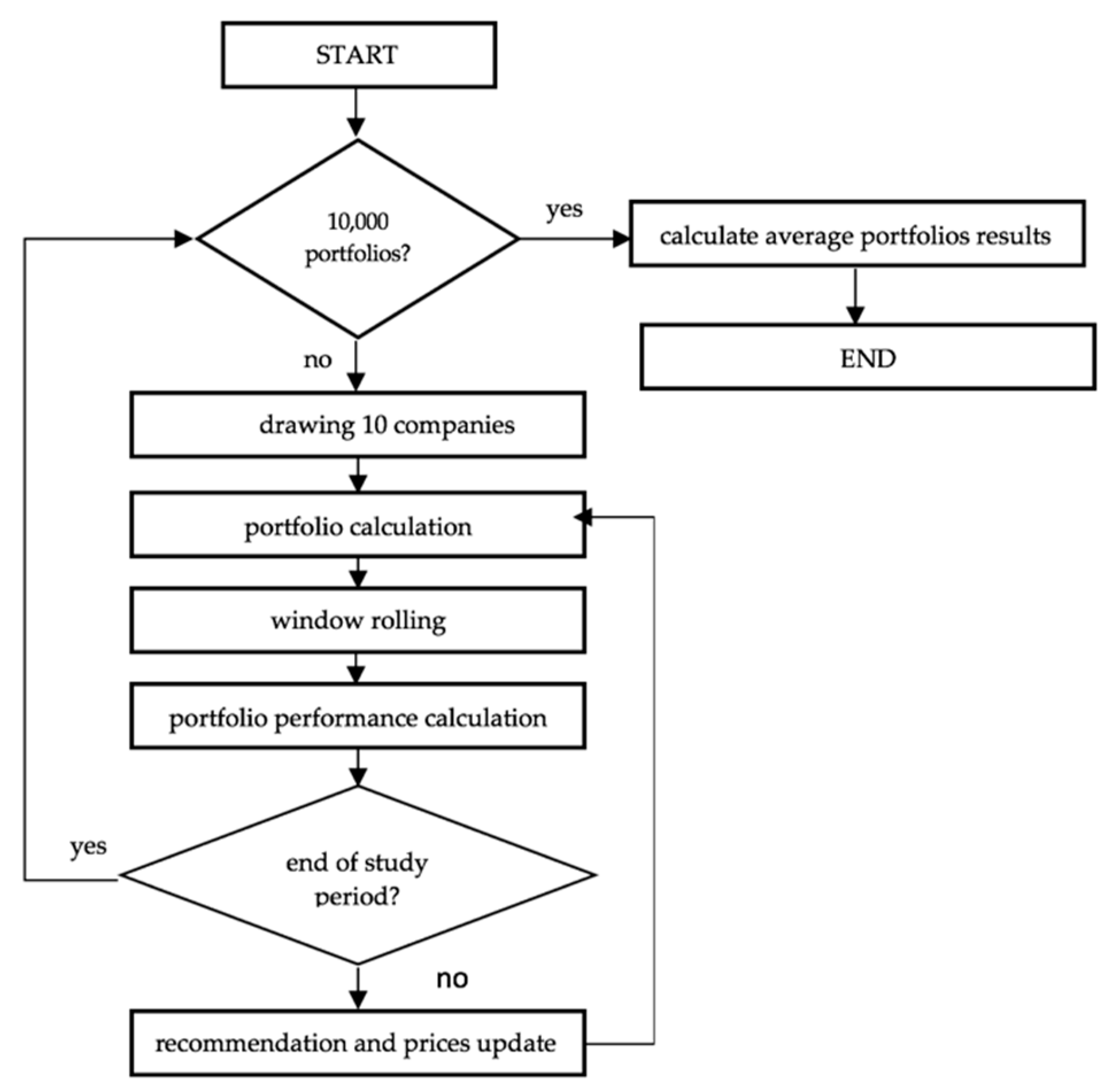
Ultimately, the procedure of this study is presented on Figure 2 and can be described as follows:
  • We draw 10 companies from the set of 29 corporations. It gives 20,030,010 possible combinations.
  • The portfolio is created from drawn companies. Five approach is used:
    • equilibrium model—CAPM (further labelled as M ),
    • standard BL model with aggregate opinions calculated as average weighted by the number of experts (further labeled as B L ),
    • fuzzy BL model with aggregate opinions with interval width 5 p.p. (fBL5),
    • fuzzy BL model with aggregate opinions with interval width 7 p.p. (fBL7),
    • fuzzy BL model with aggregate opinions with interval width 10 p.p. (fBL10).
    For each model, we have to regard 2 kinds of restrictions (with short selling and without short selling). This gives a total of 10 optimization tasks with regards to various models and to various restrictions.
  • We roll the window by 1 month.
  • For the portfolios from step 2 we calculate the rate of return.
  • We repeat steps 3 and 4 until the entire investment period runs.
  • Steps 1–5 are repeated 10,000 times.
  • We average the yields for each type of portfolio for single months
The S&P 500 index, (an American stock market index based on the market capitalizations of 500 large companies having common stock listed on the NYSE, NASDAQ, or the Cboe BZX Exchange) which can be treated as an indicator of trends in financial markets, increased by 22% in the pre-investment period and 14.7% in the investment period (Figure 3). It can be seen that in the first period the volatility is significantly lower than in the second period. Such a distinct period may affect the obtained results.

4.2. Results

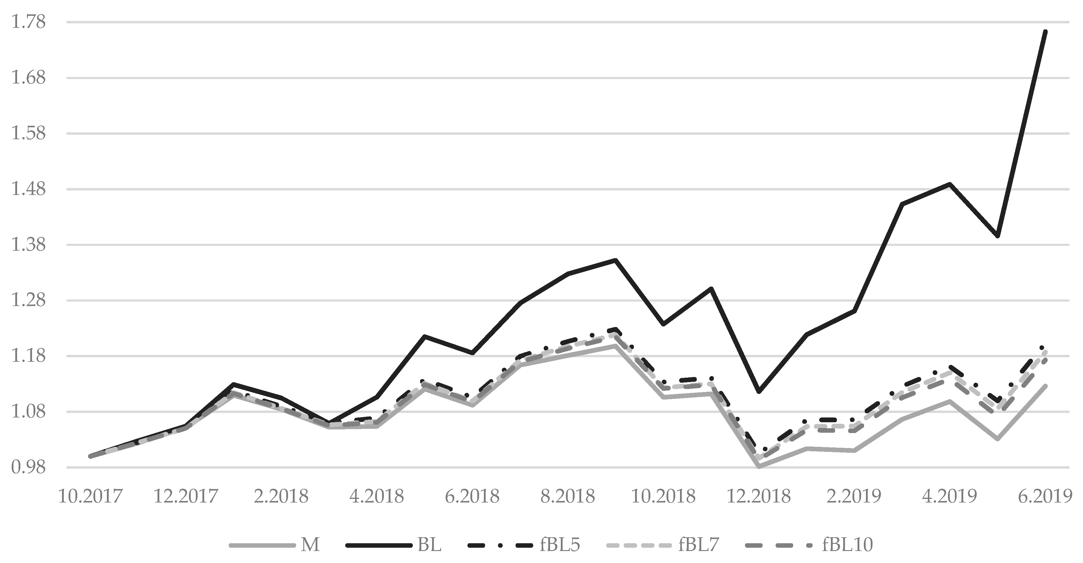
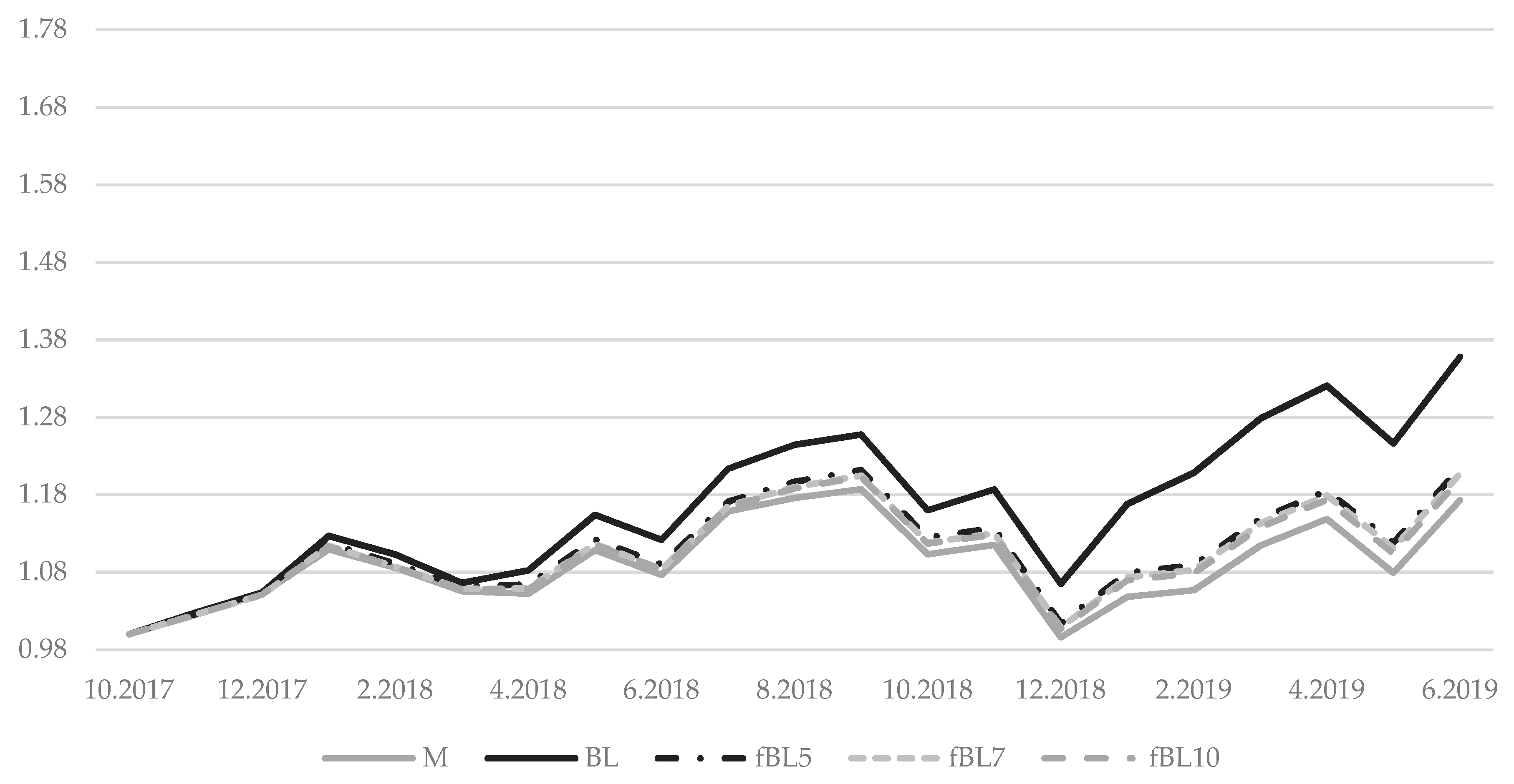
Figure 4 and Figure 5 present investment performance averaged from 10,000 portfolios in the case of investing one dollar for one year in the chosen portfolio and updated monthly according to new recommendations. It is worth noting that all models that allow us to take into account that investors’ views get better results than the equilibrium portfolio (M). As we can easily see, the inclusion of short sale allowed for higher profits in this period for each case of the BL model. This is not surprising, because a short sale allows us to get leverage. The financial leverage allows us to increase the profit, but also losses. However, a model with one or two periods with better performance quickly gains a significant advantage. Figure 4 and Figure 5 show that the intensity of changes in portfolios performance with short sale is greater than for portfolios without short sale. Nevertheless, the best results for both restrictions are achieved by standard BL portfolios. With short sale, BL portfolios’ rate of return is about 55 p.p higher than the next best portfolio. Without short sale this difference is smaller and is equal to 15 p.p. Among the fuzzy optimized portfolios, the best performance was shown to be for those that aggregate reviews with a width of 5 p.p, then those with a width of 7 p.p and 10 p.p, respectively. It is worth bearing in mind that in the case of 5 p.p. the separate intervals only touch but do not overlap. For the remaining two cases, the intervals obtained in the aggregation process have an intersection. None of the models guarantees the construction of a loss-resistant portfolio. For example, in October 2018, all portfolios generate losses. A similar situation takes place in December 2018 and May 2019.
The outstanding performance of the standard BL model with short sales is at the expense of high variability in the composition of the portfolio (Table 3). The monthly reconstruction of the portfolio requires the replacement of almost 250% of the portfolio’s value, while for the fBL models it is less than 50%. It generates costs, and in the case of large investors such replacement may be difficult or impossible. Against this background the fBL models look much better. The situation is different for models without short selling, then the BL model has a slight advantage.
An advantage of fuzzy portfolios compared to those obtained with the classic BL model is also their smaller volatility (Table 4). The performance of individual BL portfolios may differ significantly from the aforementioned average values. In the case of short sale, the risk measured by standard deviation can be up to 3 times higher. In the absence of short sale, the risk is higher by 1/3. The high volatility of BL portfolios performance is confirmed by the percentage of the best and worst portfolios (Table 5). For short sale, these portfolios have the highest percentage of best results, but they are also much more common than fuzzy ones among the worst ones. This advantage disappears for a case without a short sale.

5. Discussion

Our study focused on an empirical test of 10,000 portfolios based on recommendation from EquityRT, which were built using fuzzy modification of the Black–Litterman model. The annual average return from portfolios is 9.5–11.8% depending on the width of the intervals and additional constraints.
As previously mentioned in the literature review, studies with a fuzzy approach to views [16,18] outperform both the market portfolio and the standard BL model (by less than 3 percentage points with standard constraint and no short sells). However, it should be remembered that these studies were conducted on ex-post views. In addition, the results of portfolios built on different markets and periods are not comparable. This type of research is biased by the situation in the market. Methods that work well during prosperity are not necessarily effective when the market is bad. In the study, the BL model with short selling turned out to be the best, but at the same time it is characterized by high volatility, which is a significant flaw in market reality. The question remains whether it is a permanent feature. As mentioned, the research period, with the dominance of prices increases, may affect the results obtained. In rare periods of market decline, BL portfolios have grater losses than fuzzy models, which in turn achieve better performance than portfolios obtained from conventional optimization methods. The study is worth repeating for other periods, i.e., bear and stagnation markets. The following feature is worth noting: with narrowing the range for which expertons are created, the results are close to those obtained from the ordinary BL model.

6. Conclusions

The purpose of this study was to illustrate the method of aggregating the opinions of various experts and demonstrate the possibility of using it for real data and recommendations online. The presented approach lets one formulate intuitive views, and shows the opinions of a group of experts. The conducted experiment shows the usefulness of expertons. Expertons allow us to determine the uncertainty of views through the area under the lower and upper bound, which corresponds well with intuition.
The first advantage of the proposed solution is the ability to use opinions expressed in words, with linguistic values of the large/small type. The second, equally important, advantage is the possibility of easy and intuitive aggregation of opinions of many experts. In the case of greater uncertainty of expert opinions, a wider support of interval should be accepted. As the example shows us, this may result in a lower rate of return but a more stable portfolio. The proposed approach is of great importance for portfolio managers. It can support the decision-making process for selecting assets. However, expert knowledge is still needed, among other things, to determine reliable sources of opinions, the width of the intervals for expertons, or, last but not least, to choose a method to find the equilibrium portfolio.

Author Contributions

Conceptualization, M.B. and A.R.; methodology, M.B. and A.R.; software, M.B. and A.R.; validation, M.B. and A.R.; formal analysis, M.B. and A.R.; investigation, M.B. and A.R.; data curation, M.B. and A.R.; writing—original draft preparation, A.R.; writing—review and editing, M.B.; visualization, M.B. and A.R.; All authors have read and agreed to the published version of the manuscript.

Funding

This research received no external funding.

Conflicts of Interest

The authors declare no conflict of interest.

References

  1. Black, F.; Litterman, R. Asset Allocation: Combining Investor Views with Market Equilibrium; Discussion paper; Goldman, Sachs & Co, 1999. [Google Scholar]
  2. Black, F.; Litterman, R. Global asset allocation with equities, bonds, and currencies. Fixed Income Res. 1999, 2, 218. [Google Scholar]
  3. Goetzmann, W.N.; Brown, S.J.; Gruber, M.J.; Elton, E. Modern Portfolio Theory and Investment Analysis; John Wiley & Sons: Hoboken, NJ, USA, 2014. [Google Scholar]
  4. Levy, H. The Capital Asset Pricing Model in the 21st Century: Analytical, Empirical, and Behavioral Perspectives; Cambridge University Press: Cambridge, MA, USA, 2011. [Google Scholar] [CrossRef]
  5. He, G.; Litterman, R. The intuition behind Black-Litterman model portfolios. SSRN 1999. [Google Scholar] [CrossRef]
  6. Litterman, B. Modern Investment Management: An Equilibrium Approach; John Wiley & Sons: Hoboken, NJ, USA, 2004; Volume 246. [Google Scholar]
  7. Idzorek, T. A step-By-Step guide to the Black-Litterman model: Incorporating user-Specified confidence levels. In Forecasting Expected Returns in the Financial Markets; Satchell, S., Ed.; Academic Press: Cambridge, MA, USA, 2007; pp. 17–38. [Google Scholar]
  8. Satchell, S.; Scowcroft, A. A demystification of the Black–Litterman model: Managing quantitative and traditional portfolio construction. J. Asset Manag. 2000, 1, 138–150. [Google Scholar] [CrossRef]
  9. Walters, J. The Black-Litterman Model in Detail. SSRN 2014. [Google Scholar] [CrossRef]
  10. Meucci, A. Beyond Black-Litterman: Views on non-Normal markets. Risk 2006, 19, 87–92. [Google Scholar] [CrossRef]
  11. Giacometti, R.; Bertocchi, M.; Rachev, S.T.; Fabozzi, F.J. Stable distributions in the Black-Litterman approach to asset allocation. Quant. Financ. 2007, 7, 423–433. [Google Scholar] [CrossRef]
  12. Beach, S.L.; Orlov, A.G. An application of the Black–Litterman model with EGARCH-M-derived views for international portfolio management. Financ. Mark. Portf. Manag. 2007, 21, 147–166. [Google Scholar] [CrossRef]
  13. Bertsimas, D.; Gupta, V.; Paschalidis, I.C. Inverse optimization: A new perspective on the Black-Litterman model. Oper. Res. 2012, 60, 1389–1403. [Google Scholar] [CrossRef]
  14. Lawrence, K.D.; Pai, D.R.; Klimberg, R.K.; Lawrence, S.M. A fuzzy programming approach to financial portfolio model. In Financial Modeling Applications and Data Envelopment Applications; Lawrence, K., Kleinman, G., Eds.; Emerald Group Publishing Limited: Bingley, UK, 2009; pp. 53–59. [Google Scholar] [CrossRef]
  15. Gharakhani, M.; Sadjadi, S. A fuzzy compromise programming approach for the Black-Litterman portfolio selection model. Decis. Sci. Lett. 2013, 2, 11–22. [Google Scholar] [CrossRef]
  16. Bartkowiak, M.; Rutkowska, A. Black-Litterman Model with Multiple Experts’ Linguistic Views. In International Conference on Soft Methods in Probability and Statistics; Ferraro, M.B., Giordani, P., Vantaggi, B., Gagolewski, M., Gil, M.A., Grzegorzewski, P., Hryniewicz, O., Eds.; Springer, Cham: Berlin/Heidelberg, Germany, 2016; pp. 35–43. [Google Scholar] [CrossRef]
  17. Rutkowska, A.; Bartkowiak, M. Experton approach to vague information in portfolio selection problem with many views. In 2019 Conference of the International Fuzzy Systems Association and the European Society for Fuzzy Logic and Technology (EUSFLAT 2019); Atlantis Press: Paris, France, 2019; pp. 142–149. [Google Scholar] [CrossRef] [Green Version]
  18. Fang, Y.; Bo, L.; Zhao, D.; Wang, S. Fuzzy views on Black-Litterman portfolio selection model. J. Syst. Sci. Complex. 2018, 31, 975–987. [Google Scholar] [CrossRef]
  19. Kaufmann, A. Theory of expertons and fuzzy logic. Fuzzy Sets Syst. 1988, 28, 295–304. [Google Scholar] [CrossRef]
  20. Couturier, A.; Fioleau, B. Expertons and management decision-Making criteria interdependence and implications valuation. Fuzzy Econ. Rev. 1996, 1, 31–46. [Google Scholar] [CrossRef]
  21. Nait-Said, R.; Loukia, H. Applying the concept of experton to fuzzy mental workload modeling. Fuzzy Econ. Rev. 2003, 8, 39–63. [Google Scholar] [CrossRef]
  22. Merigó, J.M.; Lafuente, A.M.G.; Barcellos, L. Uncertain induced generalized aggregation operators and its application in the theory of expertons. Fuzzy Econ. Rev. 2010, 15, 25–43. [Google Scholar] [CrossRef]
  23. Merigó, J.M.; Casanovas, M.; Yang, J.B. Group decision making with expertons and uncertain generalized probabilistic weighted aggregation operators. Eur. J. Oper. Res. 2014, 235, 215–224. [Google Scholar] [CrossRef]
  24. Jaile-Benitez, J.M.; Ferrer-Comalat, J.C.; Linares-Mustarós, S. Determining the influence variables in the pork price, based on expert systems. In Scientific Methods for the Treatment of Uncertainty in Social Sciences; Gil-Aluja, J., Terceño-Gómez, A., Ferrer-Comalat, J.C., Merigó-Lindahl, J., Linares-Mustarós, S., Eds.; Springer, Cham: Berlin/Heidelberg, Germany, 2015; pp. 81–92. [Google Scholar] [CrossRef]
  25. Santos Caballero, A.; Gil Lafuente, J. The new Fuzzy SWOT: Empirical application with expertons. ESIC Mark. 2017, 48, 121–141. [Google Scholar] [CrossRef]
  26. Sirbiladze, G.; Khutsishvili, I.; Ghvaberidze, B. Multistage decision-Making fuzzy methodology for optimal investments based on experts’ evaluations. Eur. J. Oper. Res. 2014, 232, 169–177. [Google Scholar] [CrossRef]
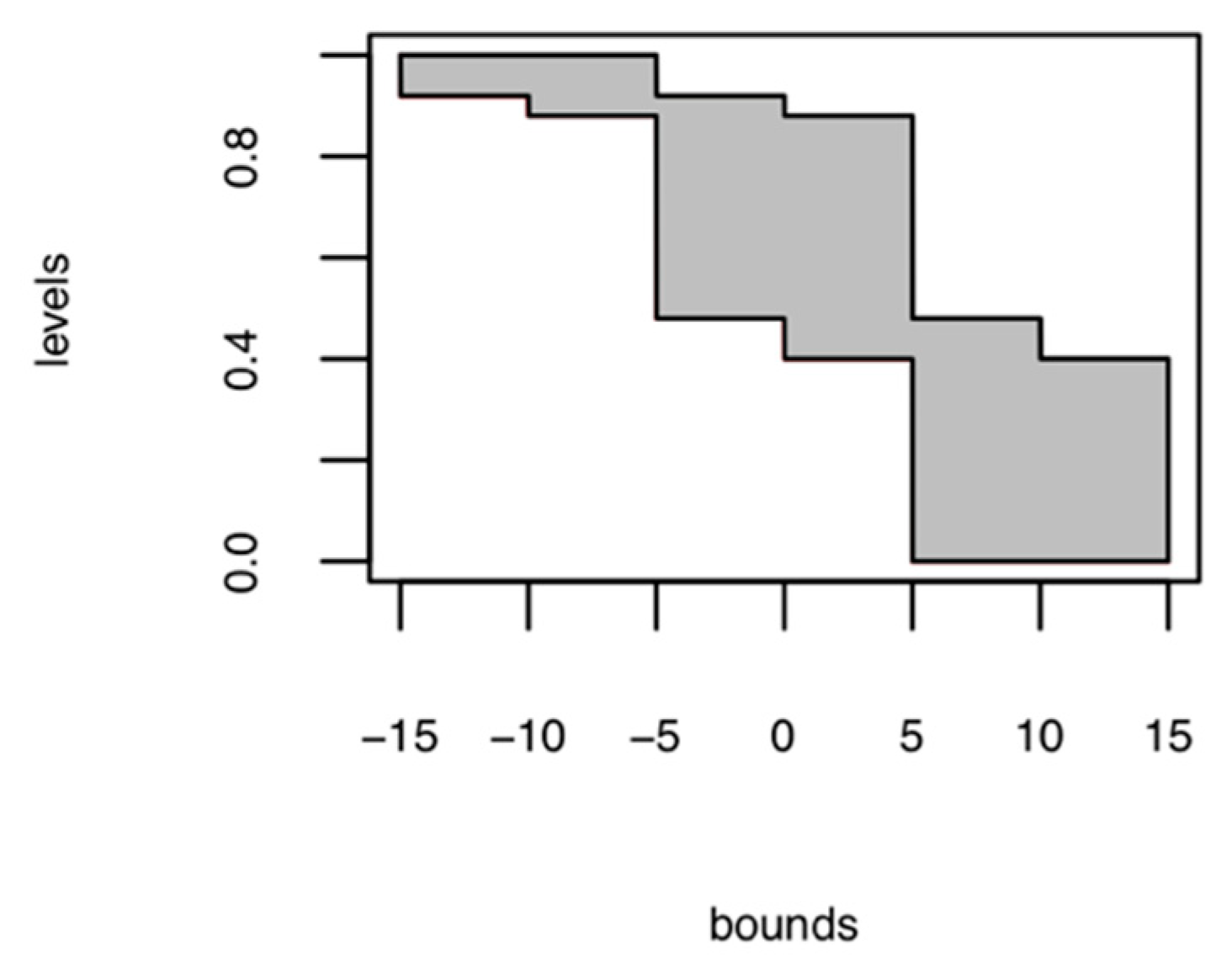
Figure 1. An experton based on experts’ recommendation for company J&J (April 2018).
Axioms 09 00038 g001
Figure 2. The procedure of empirical study.
Axioms 09 00038 g002
Figure 3. The S&P 500 index - value and the volatility (November 2016–June 2019). Volatility is obtained from the GARCH(1,1) model.
Axioms 09 00038 g003
Figure 4. Average investment performance with short sale.
Axioms 09 00038 g004
Figure 5. Average investment performance without short sale.
Axioms 09 00038 g005
Table 1. Companies analyzed in the study.
Sector
FinancialsInformation TechnologyHealth CareConsumer Discretionary
Aflac
Bank of America
Credit Acceptance
JP Morgan
Morgan Stanley
Apple
IBM
Microsoft
Visa
Bristol-Myers
Eli Lilly
Johnson & Johnson
Merck
Pfizer
Amazon
Ford
Gap
General Motors
Tesla
The Home Depot
Nike
Sector
Consumer StaplesIndustrialsEnergyCommunication ServicesMaterials
Archer Daniels
Procter & Gamble
Walmart
Boeing
Lockheed Martin
ExxonAlphabetSouthern Copper
Sector classification is consistent with Global Industry Classification Standard (GICS). This classification structure is maintained by MSCI and S&P Global Market Intelligence.
Table 2. The term-set with associated intervals.
WidthLabels
SellUnderweightHoldOverweightBuy
5 [ 12.5 , 7.5 ] [ 7.5 , 2.5 ] [ 2.5 , 2.5 ] [ 2.5 , 7.5 ] [ 7.5 , 12.5 ]
7 [ 13.5 , 6.5 ] [ 8.5 , 1.5 ] [ 3.5 , 3.5 ] [ 1.5 , 8.5 ] [ 6.5 , 13.5 ]
10 [ 15 , 5 ] [ 10 , 0 ] [ 5 , 5 ] [ 0 , 10 ] [ 5 , 15 ]
The values in brackets are given in percent.
Table 3. Average monthly change in portfolio composition.
with Short Sale
MBLfBL5fBL7fBL10
48.87%244.03%49.22%49.05%48.25%
without Short Sale
MBLfBL5fBL7fBL10
36.97%36.69%39.00%38.87%38.21%
Table 4. Standard deviation of monthly returns.
with Short Sale
MBLfBL5fBL7fBL10
7.74%22.19%8.14%7.93%7.81%
without Short Sale
MBLfBL5fBL7fBL10
6.79%10.72%7.42%7.28%7.15%
Table 5. Percentage of the best and the worst portfolios.
Percentage of the Best PortfoliosPercentage of the Worst Portfolios
with Short Sale
MBLfBL5MBLfBL5
20%58%22%44%31%25%
MBLfBL7MBLfBL7
20%59%21%44%31%24%
MBLfBL10MBLfBL10
21%60%18%44%32%24%
without Short Sale
MBLfBL5MBLfBL5
21%57%23%45%27%29%
MBLfBL7MBLfBL7
20%59%21%45%28%28%
MBLfBL10MBLfBL10
20%60%20%44%29%28%