Global Analysis and the Periodic Character of a Class of Difference Equations

Abstract

In biology, difference equations is often used to understand and describe life phenomenon through mathematical models. So, in this work, we study a new class of difference equations by focusing on the periodicity character, stability (local and global) and boundedness of its solutions. Furthermore, this equation involves a May’s Host Parasitoid Model, as a special case.

1. Introduction

The goal of our paper is to research the dynamics of solutions of equation

$$J_{n+1}=\alpha +\frac{\beta J_n^2}{\left(\gamma +J_n\right)J_{n-1}},n=0,1,\dots ,$$

(1)

where $\alpha ,\beta ,\gamma \in \left[0,\infty \right)$, $\beta \ne 0$ and the initial data $J_{-1},$$J_0\in \left(0,\infty \right)$.

When describing the evolution of any phenomenon as a mathematical model, difference equations often arise, frequently due to the discrete nature of time-evolving variable measurements and detached sciences. Difference equations are used in situations of real life, in various sciences (population models, genetics, psychology, economics, sociology, stochastic time series, combinatorial analysis, queuing problems, number theory, geometry, radiation quanta and electrical networks).

In fact, the nonlinear DEs have the efficiency to make a complicated behavior, regardless of their order. Among the well-known examples, the family $J_{n+1}=y_{\lambda }\left(J_n\right)$, $\lambda >0$, depends on $\eta$, and its conduct changes from a bounded number of periodic solutions to chaos. Due to the many applications of differential equations, there is a growing interest in searching for various aspects in terms of dynamics and behaviors of difference equations (see [1,2,3,4,5,6,7,8,9,10,11,12,13,14,15,16,17,18,19,20,21,22,23,24,25,26,27,28,29,30,31,32,33,34,35,36,37,38,39,40,41,42,43]).

Our focus in this paper is on the study of qualitative behavior of solutions of the nonlinear difference equations. Furthermore, a new equation includes a May’s Host Parasitoid Model, as a special case. Minutely, we discuss the local/global stability, boundedness and periodicity character of the solution. Moreover, by applying our results, we will prove the following cojecture:

Conjecture 1

([24]). Let $\beta >1$. Show that every positive solution of May’s Host Parasitoid Model (Equation (1) with $\alpha =0$ and $\gamma =1$) is bounded.

2. Periodic Solutions with Period $\mathit{p}$

Here, we will study the existence of periodic solutions to the Equation (1).

Theorem 1.

If $\alpha ,\beta ,\gamma \in \left[0,\infty \right)$, then Equation (1) does not have positive period two solutions. Moreover, if $\alpha ,\beta ,\gamma \in \mathbb{R}/\left\{0\right\}$ and

$$\left|\frac{1}{\beta }\left(\alpha +\beta +\gamma \right)\right|>2,$$

then Equation (1) has a period two solutions.

Proof. 

Assume that Equation (1) has a prime period two solution $\dots r,s,r,s,\dots ,\left(r\ne s\right)$. Let $\alpha ,\beta$ and $\gamma$ are nonnegative real number. From (1), we get

$$r=\alpha +\frac{\beta s^2}{\left(\gamma +s\right)r}$$

(2)

and

$$s=\alpha +\frac{\beta r^2}{\left(\gamma +r\right)s}.$$

(3)

Consequently,

$$r-s=\frac{\beta s^2}{\left(\gamma +s\right)r}-\frac{\beta r^2}{\left(\gamma +r\right)s}$$

and so

$$\left(r-s\right)\left(1+\frac{1}{rs}\frac{\beta \left(r^{2}s+\gamma r^2+r{s}^2+\gamma rs+\gamma s^2\right)}{\left(r+\gamma \right)\left(s+\gamma \right)}\right)=0.$$

Since $\alpha ,\beta ,\gamma \in \left[0,\infty \right)$, this means that $r=s$, a contradiction.

On the Other hand, if $\alpha ,\beta$ and $\gamma$ are real numbers. From (2), we get

$$\begin{array}{ccc}\hfill r& =& \alpha +\frac{\beta \frac{s}{r}}{\left(\frac{\gamma }{r}+\frac{s}{r}\right)}\frac{s}{r}\hfill \\ & =& \alpha +\frac{\beta }{t^2}\frac{1}{\left(\frac{\gamma }{r}+\frac{1}{t}\right)},\hfill \end{array}$$

where $t=r/s$. Then,

$$r^2-\left(\alpha +\frac{\beta }{t}-\gamma t\right)r-t\alpha \gamma =0,$$

which gives

$$r=\frac{1}{2t}\left(\beta +t\alpha -t^2\gamma +A\right),$$

(4)

where

$$A=\pm \sqrt{t^4{\gamma }^2+2t^3\alpha \gamma +t^2{\alpha }^2-2t^2\beta \gamma +2t\alpha \beta +{\beta }^2}.$$

Similarly, from (3), we obtain

$$s=\frac{1}{2t}\left(-\gamma +t\alpha +t^2\beta +B\right),$$

(5)

with

$$B=\pm \sqrt{t^2{\alpha }^2+t^4{\beta }^2+{\gamma }^2+2t\alpha \gamma +2t^3\alpha \beta -2t^2\beta \gamma }.$$

By using the fact $r-st=0$, (4) and (5), we find

$$A+C=Bt,$$

(6)

where

$$C=\beta +t\alpha +t\gamma -t^2\alpha -t^2\gamma -t^3\beta .$$

By simple computation, (10) shows that

$$A^4+C^4+t^4{B}^4-2A^2{B}^2{t}^2-2B^2{C}^2{t}^2+2A^2{C}^2-4A^2{C}^2=0.$$

From definitions of $A,$B and C, we have

$$t^3\alpha \gamma {\left(t-1\right)}^2{\left(\beta +t\alpha +t\beta +t\gamma +t^2\beta \right)}^2=0.$$

Since $\alpha \gamma t\ne 0$ and $t\ne 1$, we obtain

$$\frac{\alpha +\beta +\gamma }{\beta }=-\left(\frac{t^2+1}{t}\right).$$

(7)

Now, if $t\in {\mathbb{R}}^{+}$, then the function $H\left(t\right):=\left(1+t^2\right)/t$ attends its minimum value on ${\mathbb{R}}^{+}$ at $t_{+}^{*}=1$ and $H\left(t\right)>{min}_{\tau \in {\mathbb{R}}^{+}}H\left(t\right)=2$. In contrast, if $t\in {\mathbb{R}}^{-}$, then the function H attends its maximum value on ${\mathbb{R}}^{-}$ at $t_{-}^{*}=-1$ and $H\left(t\right)<{max}_{\tau \in {\mathbb{R}}^{-}}H\left(t\right)=-2$. Thus, from (7), we see that

$$\frac{1}{\beta }\left(\alpha +\beta +\gamma \right)<-2\mathrm{if}rs>0$$

or

$$\frac{1}{\beta }\left(\alpha +\beta +\gamma \right)>2\mathrm{if}rs<0.$$

The proof is complete. □

Theorem 2.

If $\alpha =0,$$\beta ,\gamma \in \mathbb{R}/\left\{0\right\}$ and either

$$\frac{\gamma }{\beta }<-3,\mathit{for}{x}_{-1}{x}_0>0,$$

or

$$\frac{\gamma }{\beta }>1,\mathit{for}{x}_{-1}{x}_0<0,$$

then Equation (1) has a period two solutions.

Proof. 

Assume that Equation (1) has a prime period two solution $\dots r,s,r,s,\dots ,\left(r\ne s\right)$. From (1), we get

$$r=\frac{\beta }{\left(\frac{\gamma }{r}+\frac{1}{t}\right)}\frac{1}{t^2},$$

where $t=r/s$. Then

$$r=\frac{\beta }{t}-\gamma t.$$

(8)

Similarly, we obtain

$$s=\beta t-\frac{\gamma }{t}.$$

(9)

By using the fact $r-st=0$, (8) and (9), we find

$$-\beta t^3-\gamma t^2+\gamma t+\beta =0,$$

and so

$$\frac{\gamma }{\beta }=-\frac{1}{t}\left(t^2+t+1\right).$$

Now, if $t\in {\mathbb{R}}^{+}$, then the function $H\left(t\right):=\left(t^2+t+1\right)/t$ attends its minimum value on ${\mathbb{R}}^{+}$ at $t_{+}^{*}=1$ and $H\left(t\right)>{min}_{\tau \in {\mathbb{R}}^{+}}H\left(t\right)=3$. In contrast, if $t\in {\mathbb{R}}^{-}$, then the function H attends its maximum value on ${\mathbb{R}}^{-}$ at $t_{-}^{*}=-1$ and $H\left(t\right)<{max}_{\tau \in {\mathbb{R}}^{-}}H\left(t\right)=-1$. Thus, from (7), we se that

$$\frac{\gamma }{\beta }<-3\mathrm{if}rs>0$$

or

$$\frac{\gamma }{\beta }>1\mathrm{if}rs<0.$$

The proof is complete. □

Theorem 3.

Let p be a positive integer and $p>2$. If every positive solution of Equation (1) is periodic with period p, then $\alpha =0$.

Proof. 

Assume that every positive solution of Equation (1) is periodic with period p. Now, we consider the solution with

$$J_{-1}=1\mathrm{and}{J}_0\in \left(0,\infty \right).$$

Hence, $J_{p-1}=1$ and $J_p=J_0$. From Equation (1), we have

$$\begin{array}{ccc}\hfill J_p& =& \alpha +\frac{\beta J_{p-1}^2}{\left(\gamma +J_{p-1}\right)J_{p-2}}\hfill \\ & =& \alpha +\frac{\beta }{\left(\gamma +1\right)J_{p-2}}=J_0,\hfill \end{array}$$

or

$$\alpha \left(\gamma +1\right)J_{p-2}+\beta =\left(\gamma +1\right)J_0{J}_{p-2}.$$

Assume that $\alpha \ne 0$ and $\beta >0$. If we choose $J_0<\alpha$, then

$$\begin{array}{ccc}\hfill \alpha \left(\gamma +1\right)J_{p-2}+\beta & =& \left(\gamma +1\right)J_0{J}_{p-2}\hfill \\ & <& \alpha \left(\gamma +1\right)J_{p-2}\hfill \end{array}$$

which is impossible and hence $\alpha =0$. The proof of the theorem is complete. □

Remark 1.

Let $\alpha =0$, it is possible that every positive solution of Equation (1) is periodic with period p. As a special case, if $\alpha =\gamma =0$, then we see that every positive solution of equation

$$J_{n+1}=\beta \frac{J_n}{J_{n-1}}$$

is periodic with period six

$$J_{-1},J_0,\beta \frac{J_0}{J_{-1}},{\beta }^2\frac{1}{J_{-1}},{\beta }^2\frac{1}{J_0},\beta \frac{J_{-1}}{J_0},\dots .$$

3. Stability and Boundedness

Let $J_e$ be a point in the domain of the function F. Then, $J_e$ is said to be an equilibrium point of equation $J_{n+1}=F\left(J_n,J_{n-1}\right)$ if $J_e$ is a fixed point of F, i.e., $F\left(J_e,J_e\right)=J_e$. The idea of equilibrium points (states) is focal in the investigation of the dynamics of any physical system. In numerous applications in science, physics, engineering, and so on., it is known that all states (solutions) of a given system tend to its equilibrium state (point). We presently give the formula of an equilibrium point of Equation (1). To find the positive equilibrium points, we let $F\left(J_e,J_e\right)=J_e$, or

$$J_e=\alpha +\frac{\beta J_e^2}{\left(\gamma +J_e\right)J_e}$$

and so

$$J_e^2-\left(\alpha +\beta -\gamma \right)J_e-\alpha \gamma =0.$$

Thus, we have both cases:

Case (1): If $\alpha +\beta =\gamma$, then the only positive equilibrium point is

$$J_e=\sqrt{\alpha \gamma }.$$

Case (2): If $\alpha +\beta \ne \gamma$, then the only positive equilibrium point is

$$J_e=\frac{1}{2}\left(\alpha +\beta -\gamma \right)+\frac{1}{2}\sqrt{{\left(\alpha +\beta -\gamma \right)}^2+4\alpha \gamma }.$$

Also, if $\alpha \gamma =0$, then the only positive equilibrium is

$$J_e=\alpha +\beta -\gamma ,\mathrm{if}\alpha +\beta >\gamma .$$

One of the fundamental objectives in the investigation of a dynamical system is to determine the behavior of its solutions near an equilibrium point. For the basic definitions of stability see [24]. To study the local stability of a positive equilibrium point, we define the function $F:\left(0,\infty \right)\times \left(0,\infty \right)\to \left(0,\infty \right)$ by

$$F\left(u,v\right)=\alpha +\frac{\beta u^2}{\left(\gamma +u\right)v}.$$

(10)

The partial derivatives of function F are

$$\frac{\partial }{\partial u}F\left(u,v\right)=\frac{u}{v}\frac{\beta }{{\left(u+\gamma \right)}^2}\left(u+2\gamma \right)$$

(11)

and

$$\frac{\partial }{\partial v}F\left(u,v\right)=-\frac{u^2}{v^2}\frac{\beta }{u+\gamma }.$$

(12)

The equilibrium point $J_e$ is called a sink or an attracting equilibrium if every eigenvalue of Jacobian matrix of $J_e$ has absolute value less than $one$, see [23]. In the following theorem, by using Theorem 1.1.1 in [24], we study a locally asymptotically stable for positive equilibrium point of (1) when $\alpha ,\beta ,\gamma \in \left[0,\infty \right)$.

Theorem 4.

Let $\alpha \ne 0$. Then the positive equilibrium point of Equation (1) is locally asymptotically stable and sink.

Proof. 

By replacing both u and v with $J_e$ in Equations (11) and (12), we get

$$\frac{\partial }{\partial u}F\left(J_e,J_e\right)=\frac{\beta }{{\left(\gamma +J_e\right)}^2}\left(2\gamma +J_e\right):={\mu }_u$$

(13)

and

$$\frac{\partial }{\partial v}F\left(J_e,J_e\right)=-\frac{\beta }{\gamma +J_e}:={\mu }_v.$$

(14)

Then, the linearized equation associated with (1) about $J_e$ is

$$z_{n+1}-{\mu }_u{z}_n-{\mu }_v{z}_{n-1}=0.$$

Now, we have

$$\begin{array}{ccc}\hfill J_e& =& \frac{1}{2}\left(\alpha +\left(\beta -\gamma \right)\right)+\frac{1}{2}\sqrt{{\left(\alpha +\left(\beta -\gamma \right)\right)}^2+4\alpha \gamma }\hfill \\ & >& \left(\frac{1}{2}+\frac{1}{2}\right)\left(\beta -\gamma \right)\hfill \end{array}$$

and so

$$\frac{\beta }{\gamma +J_e}<1.$$

Moreover, we see that

$$\frac{\beta \gamma }{{\left(\gamma +J_e\right)}^2}<\frac{\gamma }{\gamma +J_e}<1.$$

(15)

From (13)–(15), we obtain

$$\begin{array}{ccc}\hfill \left|{\mu }_u\right|+{\mu }_v& =& \frac{\beta }{{\left(\gamma +J_e\right)}^2}\left(2\gamma +J_e\right)-\frac{\beta }{\gamma +J_e}\hfill \\ & =& \frac{\beta \gamma }{{\left(\gamma +J_e\right)}^2}<1\hfill \end{array}$$

and

$${\mu }_v=-\frac{\beta }{\gamma +J_e}>-1.$$

Hence, we have $\left|{\mu }_u\right|<1-{\mu }_v<2$. Therefore, $J_e$ is locally asymptotically stable and sink. The proof of the theorem is complete. □

Theorem 5.

Let $\alpha =0$ and $\beta >\gamma$. Then the positive equilibrium point of Equation (1) is locally asymptotically stable and sink.

Proof. 

The proof is similar to the proof of Theorem 4 and so we omit it. □

Lemma 1.

If $\alpha >0$, then

$$\alpha <J_n\le \alpha +\beta \left(1+\frac{\beta }{\alpha }\right),$$

(16)

for all $n>0$ and so every solution of Equation (1) is bounded.

Proof. 

Suppose that ${\left\{J_n\right\}}_{n=-1}^{\infty }$ be a solution of (1). It follows from (1) that

$$J_{n+1}=\alpha +\frac{\beta J_n^2}{\left(\gamma +J_n\right)J_{n-1}}>\alpha .$$

Since $\gamma >0,$ we have $J_n<\gamma +J_n$, and thus

$$\begin{array}{ccc}\hfill J_{n+1}& =& \alpha +\frac{\beta J_n^2}{\left(\gamma +J_n\right)J_{n-1}}\hfill \\ & =& \alpha +\beta \frac{J_n}{\left(\gamma +J_n\right)}\frac{J_n}{J_{n-1}}\hfill \end{array}$$

$$\begin{array}{cc}<& \alpha +\beta \frac{J_n}{J_{n-1}}.\hfill \end{array}$$

(17)

Next, we let

$${\varphi }_{n+1}=\alpha +\beta \frac{{\varphi }_n}{{\varphi }_{n-1}}.$$

(18)

From (18), we get ${\varphi }_n>\alpha$ for all $n>1$, and so

$$\begin{array}{ccc}\hfill {\varphi }_{n+1}& =& \alpha +\beta \left(\frac{\alpha }{{\varphi }_{n-1}}+\frac{\beta }{{\varphi }_{n-2}}\right)\hfill \\ & <& \alpha +\beta \left(1+\frac{\beta }{\alpha }\right).\hfill \end{array}$$

Thus, and from (17), we get

$$\alpha <J_n<\alpha +\beta \left(1+\frac{\beta }{\alpha }\right),$$

for all $n>1$. The proof of the lemma is complete. □

Lemma 2.

If $\alpha =0$ and $\beta >\gamma$, then all solution of (1) is bounded.

Proof. 

As in the proof of Lemma 1, (17) holds. If $\alpha =0$, then (17) becomes

$$J_{n+1}<\beta \frac{J_n}{J_{n-1}}.$$

Moreover, every positive solution of equation $y_{n+1}=\beta y_n/y_{n-1}$ is periodic with period six $\{y_{-1},$$y_0,$$\beta y_0/y_{-1},$${\beta }^2/y_{-1},$${\beta }^2/y_0,$$\beta y_{-1}/y_0\}$. Thus,

$$0<J_{n+1}<max\left\{J_{-1},J_0,\beta \frac{J_0}{J_{-1}},{\beta }^2\frac{1}{J_{-1}},{\beta }^2\frac{1}{J_0},\beta \frac{J_{-1}}{J_0}\right\}.$$

The proof of the lemma is complete. □

Theorem 6.

Assume that $\alpha \ne 0$, $\gamma >\beta$ and ${\alpha }^6>2\beta \gamma {\left({\alpha }^2+\alpha \beta +{\beta }^2\right)}^2$. Then (1) has a unique equilibrium $J_e$ and every solution of (1) converges to $J_e$.

Proof. 

Consider the function F defined as (10). From (11) and (12), we have that F is increasing in u and decreasing in v. Now, let $\left(U,L\right)$ be a solution of the system

$$\left\{\begin{array}{c}J=F\left(J,y\right);\\ y=F\left(y,J\right).\end{array}\right.$$

Then, we get

$$U=\alpha +\frac{\beta U^2}{\left(\gamma +U\right)L}$$

and

$$L=\alpha +\frac{\beta L^2}{\left(\gamma +L\right)U}.$$

Hence, we have

$$\begin{array}{ccc}\hfill U-L& =& \frac{\beta U^2}{\left(\gamma +U\right)L}-\frac{\beta L^2}{\left(\gamma +L\right)U}\hfill \\ & =& \left(U-L\right)\frac{\beta \left(L^{2}U+\gamma L^2+L{U}^2+\gamma LU+\gamma U^2\right)}{LU\left(L+\gamma \right)\left(U+\gamma \right)}\hfill \end{array}$$

and

$$\left(U-L\right)\left(1-\frac{\beta \gamma \left(L^2+U^2\right)+\beta \left(L^{2}U+L{U}^2+\gamma LU\right)}{L^2{U}^2+\gamma \left(L^{2}U+L{U}^2+\gamma LU\right)}\right)=0.$$

(19)

From Lemma 1, we have

$$\alpha <L,U<\alpha +\beta \left(1+\frac{\beta }{\alpha }\right).$$

Thus, and from $2\beta \gamma {\left({\alpha }^2+\alpha \beta +{\beta }^2\right)}^2<{\alpha }^6$, we get

$$\begin{array}{ccc}\hfill \beta \gamma \left(L^2+U^2\right)& <& 2\beta \gamma {\left(\alpha +\beta \left(1+\frac{\beta }{\alpha }\right)\right)}^2\hfill \\ & =& \frac{2}{{\alpha }^2}\beta \gamma {\left({\alpha }^2+\alpha \beta +{\beta }^2\right)}^2\hfill \\ & <& {\alpha }^4\hfill \\ & <& L^2{U}^2.\hfill \end{array}$$

Since $\gamma >\beta$, we find

$$\frac{\beta \gamma \left(L^2+U^2\right)+\beta \left(L^{2}U+L{U}^2+\gamma LU\right)}{L^2{U}^2+\gamma \left(L^{2}U+L{U}^2+\gamma LU\right)}<1.$$

(20)

From (19) and (20), we obtain $L=U$. From Theorem 1.4.5 in [24], we have that all solution of (1) converges to $J_e$. The proof of the theorem is complete. □

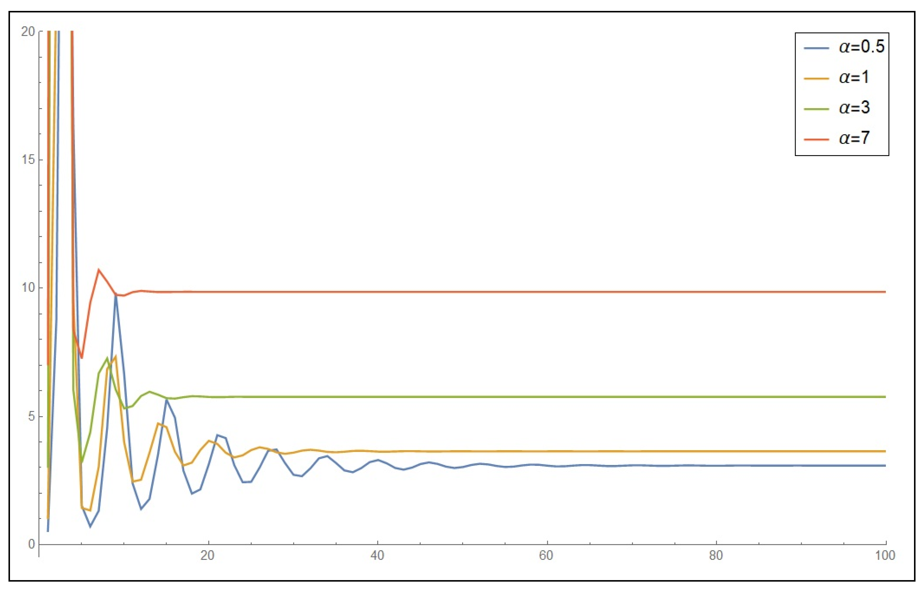
4. Application and Discussion

In Equation (1), if $\alpha =0$ and $\gamma =1$, we get the May’s Host Parasitoid Model

$$J_{n+1}=\frac{\beta J_n^2}{\left(1+J_n\right)J_{n-1}}.$$

(21)

By using Theorems 1 and 5 and Lemma 2, respectively, we get the following corollaries:

Corollary 1.

Model (21) does not have positive period two solutions.

Corollary 2.

Assume that $\beta >1$. The positive equilibrium point of equation $J_e=\left(\beta -1\right)$ of model (21) is locally asymptotically stable and sink.

Corollary 3.

If $\beta >1$, then every solution of model (21) is bounded.

Remark 2.

Note that, Corollaries 1–3 gave some qualitative behaviors of the model (21). Moreover, Corollary 3 confirms the Conjecture 1.

Example 1.

Let the equation

$$J_{n+1}=\alpha +\frac{3J_n^2}{\left(0.5+J_n\right)J_{n-1}}.$$

(22)

Figure 1 shows the dynamics of (22) with $J_{-1}=1.5$ and $J_0=0.1$. Let $N_e$ be the first value of n in which the solution is stable (by approximation ${10}^{-6}$), for example, let $\alpha =1$, we have

n	…	89	90	91	92	…
Jn	…	3.63746	3.63745	3.63745	3.63745	…

So, $N_e=90$. Note that,

α	0.5	1	3	7
Ne	150	90	43	28
Je	3.08114	3.63745	5.76040	9.85514

Remark 3.

Note that, when the value of α increases, stability occurs faster.

References

1. Abdelrahman, M.A.E.; Chatzarakis, G.E.; Li, T.; Moaaz, O. On the difference equation Jn+1 = aJn−l + bJn−k + f(Jn−l, Jn−k). Adv. Differ. Equ. 2018, 431, 2018. [Google Scholar]
2. Agarwal, R.P.; Elsayed, E.M. Periodicity and stability of solutions of higher order rational difference equation. Adv. Stud. Contemp. Math. 2008, 17, 181–201. [Google Scholar]
3. Ahlbrandt, C.D.; Peterson, A.C. Discrete Hamiltonian Systems: Difference Equations, Continued Fractions, and Riccati Equations; Kluwer Academic Publishers: Dordrecht, The Netherlands, 1996. [Google Scholar]
4. Ahmad, S. On the nonautonomous Volterra-Lotka competition equations. Proc. Am. Math. Soc. 1993, 117, 199–204. [Google Scholar] [CrossRef]
5. Allman, E.S.; Rhodes, J.A. Mathematical Models in Biology: An Introduction; Cambridge University Press: Cambridge, UK, 2003. [Google Scholar]
6. Andres, J.; Pennequin, D. Note on Limit-Periodic Solutions of the Difference Equation xt+1 − [h(xt) + λ]x = rt,λ > 1. Axioms 2019, 8, 19. [Google Scholar] [CrossRef]
7. Din, Q.; Elsayed, E.M. Stability analysis of a discrete ecological model. Comput. Ecol. Soft. 2014, 4, 89–103. [Google Scholar]
8. Grove, E.A.; Ladas, G. Periodicities in Nonlinear Difference Equations; Chapman & Hall/CRC: Boca Raton, FL, USA, 2005; Volume 4. [Google Scholar]
9. Elabbasy, E.M.; El-Metwally, H.; Elsayed, E.M. On the difference equation Jn+1 = (aJn−l + bJn−k)/(cJn−l + dJn−k). Acta Math. Vietnam. 2008, 33, 85–94. [Google Scholar]
10. Elabbasy, E.M.; Elsayed, E.M. Dynamics of a rational difference equation. Chin. Ann. Math. Ser. B 2009, 30, 187–198. [Google Scholar] [CrossRef]
11. El-Dessoky, M.M. On the difference equation Jn+1 = aJn−l + bJn−k + cJn−s/(dJn−se). Math. Methods Appl. Sci. 2016, 1, 082579. [Google Scholar]
12. Elettreby, M.F.; El-Metwally, H. On a system of difference equations of an economic model. Discret. Dyn. Nat. Soc. 2013, 2013, 405628. [Google Scholar] [CrossRef]
13. Elsayed, E.M. Dynamics and behavior of a higher order rational difference equation. J. Nonlinear Sci. Appl. 2015, 9, 1463–1474. [Google Scholar] [CrossRef]
14. Elsayed, E.M. New method to obtain periodic solutions of period two and three of a rational difference equation. Nonlinear Dyn. 2015, 79, 241–250. [Google Scholar] [CrossRef]
15. Elsayed, E.M.; Iricanin, B.D. On a max-type and a min-type difference equation. Appl. Math. Comput. 2009, 215, 608–614. [Google Scholar] [CrossRef]
16. Elsayed, E.M.; El-Dessoky, M.M. Dynamics and behavior of a higher order rational recursive sequence. Adv. Differ. Equ. 2012, 69, 2012. [Google Scholar] [CrossRef]
17. Foupouagnigni, M.; Mboutngam, S. On the Polynomial Solution of Divided-Difference Equations of the Hypergeometric Type on Nonuniform Lattices. Axioms 2019, 8, 47. [Google Scholar] [CrossRef]
18. Foupouagnigni, M.; Koepf, W.; Kenfack-Nangho, M.; Mboutngam, S. On Solutions of Holonomic Divided-Difference Equations on Nonuniform Lattices. Axioms 2013, 2, 404–434. [Google Scholar] [CrossRef]
19. Gil, M. Solution Estimates for the Discrete Lyapunov Equation in a Hilbert Space and Applications to Difference Equations. Axioms 2019, 8, 20. [Google Scholar] [CrossRef]
20. Haghighi, A.M.; Mishev, D.P. Difference and Differential Equations with Applications in Queueing Theory; John Wiley & Sons Inc.: Hoboken, NJ, USA, 2013. [Google Scholar]
21. Kalabusic, S.; Kulenovic, M.R.S. On the recursive sequnence Jn+1 = (αJn−1 + βJn−2)/(γJn−1 + δJn−2). J. Differ. Equ. Appl. 2003, 9, 701–720. [Google Scholar]
22. Kelley, W.G.; Peterson, A.C. Difference Equations: An Introduction with Applications, 2nd ed.; Harcour Academic: New York, NY, USA, 2001. [Google Scholar]
23. Kocic, V.L.; Ladas, G. Global Behavior of Nonlinear Difference Equations of Higher Order with Applications; Kluwer Academic Publishers: Dordrecht, The Netherlands, 1993. [Google Scholar]
24. Kulenovic, M.R.S.; Ladas, G. Dynamics of Second Order Rational Difference Equations with Open Problems and Conjectures; Chapman & Hall/CRC Press: Boca Raton, FL, USA, 2001. [Google Scholar]
25. Liu, X. A note on the existence of periodic solutions in discrete predator-prey models. Appl. Math. Model. 2010, 34, 2477–2483. [Google Scholar] [CrossRef]
26. Ma, W.-X. Global behavior of a new rational nonlinear higher-order difference equation. Complexity 2019, 2019, 2048941. [Google Scholar] [CrossRef]
27. Migda, M.; Migda, J. Nonoscillatory Solutions to Second-Order Neutral Difference Equations. Symmetry 2018, 10, 207. [Google Scholar] [CrossRef]
28. Moaaz, O. Comment on new method to obtain periodic solutions of period two and three of a rational difference equation [Nonlinear Dyn 79: 241–250]. Nonlinear Dyn. 2017, 88, 1043–1049. [Google Scholar] [CrossRef]
29. Moaaz, O. Dynamics of difference equation Jn+1 = f(Jn−l, Jn−k). Adv. Differ. Equ. 2018, 447, 2018. [Google Scholar]
30. Moaaz, O.; Chalishajar, D.; Bazighifan, O. Some Qualitative Behavior of Solutions of General Class of Difference Equations. Mathematics 2019, 7, 585. [Google Scholar] [CrossRef]
31. Pogrebkov, A. Hirota Difference Equation and Darboux System: Mutual Symmetry. Symmetry 2019, 11, 436. [Google Scholar] [CrossRef]
32. Stevic, S. On the recursive sequance xn+1 = α + x n 1 p / x n p . J. Appl. Math. Comput. 2005, 18, 229–234. [Google Scholar]
33. Stevic, S.; Kent, C.; Berenaut, S. A note on positive nonoscillatory solutions of the differential equation xn+1 = α + x n 1 p / x n p . J. Diff. Eqs. Appl. 2006, 12, 495–499. [Google Scholar]
34. Stevic, S. On the recursive sequence xn+1 = αn + xn−1/xn. Dynam. Contin. Discret. Impuls. Syst. Ser. A Math. Anal. 2003, 10, 911–917. [Google Scholar]
35. Stevic, S. A note on periodic character of a difference equation. J. Differ. Equ. Appl. 2004, 10, 929–932. [Google Scholar] [CrossRef]
36. Stevic, S. A short proof of the Cushing–Henson conjecture. Discret. Dyn. Nat. Soc. 2006, 4, 37264. [Google Scholar] [CrossRef]
37. Stevic, S. Global stability and asymptotics of some classes of rational difference equations. J. Math. Anal. Appl. 2006, 316, 60–68. [Google Scholar] [CrossRef]
38. Stevic, S. Asymptotics of some classes of higher order difference equations. Discret. Dyn. Nat. Soc. 2007, 2007, 56813. [Google Scholar] [CrossRef]
39. Stevic, S. Asymptotic periodicity of a higher order difference equation. Discret. Dyn. Nat. Soc. 2007, 2007, 13737. [Google Scholar] [CrossRef]
40. Stevic, S. Existence of nontrivial solutions of a rational difference equation. Appl. Math. Lett. 2007, 20, 28–31. [Google Scholar] [CrossRef]
41. Taousser, F.Z.; Defoort, M.; Djemai, M.; Djouadi, S.M.; Tomsovic, K. Stability analysis of a class of switched nonlinear systems using the time scale theory. Nonlinear Anal. Hybrid Syst. 2019, 33, 195–210. [Google Scholar] [CrossRef]
42. Wang, C.; Agarwal, R.P. Almost periodic solution for a new type of neutral impulsive stochastic Lasota–Wazewska timescale model. Appl. Math. Lett. 2017, 70, 58–65. [Google Scholar] [CrossRef]
43. Yang, C. Positive Solutions for a Three-Point Boundary Value Problem of Fractional Q-Difference Equations. Symmetry 2018, 10, 358. [Google Scholar] [CrossRef] [Green Version]
Figure 1. The stable solution of Equation (22) when α = 0.5 , 1 , 3 and 7.
Axioms 08 00131 g001