1. Introduction
In recent years, in the automotive industry, the electric motors market has grown. The attention about the environment and the renewable energy has led to the electrification of road transport [
1,
2,
3]. Nowadays, one of the challenges is the reduction of carbon dioxide emissions [
4]. The use of an electric motor has brought more advantage; motor life is increased because it contains relatively few moving parts. In general, automated controls are easily integrated to operate electric motors providing the versatility of automatic functions [
5]. The main advantage of these machines is their high efficiency due to the absence of field-coil losses. Different types of classification could be done related to the new vehicles that are based on the chosen motor, the design of their permanent magnets, the energy system and source, and the configuration of the power transmission inside the Electric Vehicles in general (EV) [
6,
7]. The vehicle architectures vary every day, and the state of art is fusing on power coming from the classic Internal Combustion Engine (ICE) with the innovative electric thrust. This paper presents the configuration of a mild hybrid electric vehicles (MHEVs). MHEVs are vehicles where propulsion energy is available from more than one type of energy stores, sources, or converters, and at least one of them can deliver electrical energy. The significant features on EVs are the electrical power available, the fuel consumption, the functions performed, and the battery voltage. At the end of the paper, the results will show the difference about fuel consumption between the standard driving cycles. To measure the level of the MHEVs and to give a view of the dynamic performance of the vehicle, the hybridization factor (HF) is used in the simulation, which express the quantity of power provided by the electric part versus the total employed (1), where
is the power of electric motor and
is the power of ICE (Internal Combustion Engine):
The advantages of MHEVs are lower emissions, higher fuel economy, durability, and reliability, but the major issue for these is the integration with ICE components, medium costs, and the dimension of the battery pack. The effects of the control applied, depending on the model accuracy, so the highly non-linearity behavior of the motor must be considered [
8,
9]. Generally, this phenomenon is described and controlled, employing techniques to achieve more precise results. A Model Predictive Control (MPC) leads to higher efficiency when compared to conventional controls [
10,
11].
2. Control Algorithms
A MHEV system is a complex system that is made by different components: motors, battery, converter, gear, and transmission. The electric motor control techniques are the same, even if the attached components are different. There are consolidated control strategies, and the principal used is related to direct torque control (DTC) and vector control (called also field oriented control, FOC) instead of the old scalar control. These methods that are applied to motors are mainly used for speed and torque control. Analysis and comparison of the results show that the two control techniques provide good performances, with a faster dynamic torque in the case of direct torque control and better behavior in the permanent mode for the FOC. At present, high-performance speed and torque control techniques are classified into two main categories: Vector control (VC) and Direct torque control (DTC).
Scalar Control. It is indicated by the term “scalar control”, in that the control device determines either only the amplitude and the frequency of the voltage to be applied to the stator circuit. Scalar control is based on the steady-state model of the motor. The control is due to the magnitude variation of the control variables only and it disregards the coupling effect in the machine (the voltage of a motor can be controlled to control the flux, and frequency or slip can be controlled to control the torque). Motor voltage and the frequency of its phase currents both simultaneously affect and control both magnetic flux and electromagnetic torque of the motor. This method is simple and easy to implement, but the inherent coupling effect (i.e., both torque and flux are functions of voltage or current and frequency) gives a sluggish response, and the system is prone to instability due to a high-order (fifth-order) system effect. As a result, the scalar control technique has poor dynamic performance. The scalar controller is usually used in low-cost and low-performance drives; it is the simplest control and usually is not used with feedback [
12,
13] If the frequency decreases or the voltage increases, the coils can be burned, or saturation can occur in the iron of coils. It is necessary to vary the frequency and the voltage at the same time to avoid these problems. According to the equation of induced voltage, the V/Hz constant control gives constant flux in the stator. It uses a voltage supply of the stator winding of the machine [
14].
Direct torque control. A control technique highly used in the last decade, is Direct Torque Control (DTC) [
15,
16]. Torque and stator and rotor flux are directly controlled. in this method. The main advantages are fast dynamic torque response; high ripple and distortion of steady-state torque, flux, current; average complexity of implementation; and, no need transformation or PWM modulator but the use of hysteresis bands like a regulator. DTC strategies allow for direct control of motor variables through an appropriate selection of the inverter control signals, in order to fulfill the requirements as the electromagnetic torque needs to be increased or decreased. The two primary schemes in this kind of direct control are the traditional switching table and the space vector modulation, like the Direct Self Torque Control (DSTC), which has hexagonal trajectory proposed in [
17]. An interesting DTC strategy is presented on [
18], which is based on the one introduced before with two significant improvements. The first one is aimed at the drive reliability improvement. This has been carried out through the application of appropriate null voltage vectors to achieve the control signal in an attempt to equilibrate the switching frequencies of the inverter and eliminate the common mode voltage (CMV) drawbacks. The second modification is based on the substitution of the two-level hysteresis controller in the torque loop by a three-level one to achieve the application of active voltage vectors corresponding to the three-phase conduction mode during sector-to-sector commutations. The paper offers an interesting novel DTC strategy that is dedicated to the control of brushless DC (BLDC) motor drives. Unlike traditional vector control, DTC does not require coordinate transformation, PI regulators, pulse width modulation (PWM), and position encoders. Hence, DTC is much simpler. Moreover, both DTC and VC provide a good dynamic response, but DTC is less sensitive to the motor parameter variations.
Vector Control. Also called field-oriented control, it provides a current supply. It is identified by the term “vector control”, in that the control block determines the value of the module and the direction of the current vector to be applied to the machine stator or, equivalently, its two components to be applied according to an appropriate reference system. The field-oriented control is based on appropriate selection of the reference axes used by the regulator in such a way that one component of the stator current acts exclusively on the flow, and the other on the torque of the electric machine (Park′s transformation). In this way, the asynchronous machine is regulated as an independent excitation current machine, in which the excitation current and the armature current (rotor) are separately operated. The field-oriented control ensures functional and robust control in the case of transients, and it is based on a mathematical abstraction. With this technique, it is possible to uncouple the field components. Uncoupling establishes two independent and single controlled currents: the flux producing current and the torque producing current and high-performance drive can be realized. Field oriented control is also characterized by low values of the ripples of currents and electromagnetic torque when compared to with the direct torque control.
The authors simulated control solution. In the last years, the authors chose to simulate/emulate a complete vehicle where the electric motor control could be driven by a FOC or DTC. Different techniques are present in literature in order to filter the noise, the road effect, or the vehicle’s dynamic effects (sliding mode, predictive estimation, and adaptive control [
19,
20,
21,
22,
23,
24,
25]). Authors choose to filter the reference given by the driver with a model predictive control scheme.
The experimental results confirm that the high speed of detection provided by this approach allows for a satisfactory transition from pre-fault to post-fault mode of operation, even using this sensitive strategy.
On the simulated vehicle, the Model Predictive Controller (MPC) has been directly applied in the electric motor control unit. The MPC is designed in dimensionless form, as follows:
where
, B, C, and D are the constant state-space matrices;
is a diagonal matrix of input scale factors;
is a diagonal matrix of output;
is the state vector;
is the vector of plant input variables; and,
is the vector of plant output variables. The resulting plant model has the following equivalent form:
where
,
,
, and
are the columns of
.
,
, and
are the columns of
.
is the manipulated variables,
is the measured disturbances, and
is the unmeasured input disturbances.
3. Vehicle′s Architecture and Mathematical Model
MHEVs are growing, given the increasingly restrictive limits. As a result of rising environmental concerns and available resource limitations of oil, it has become imperative on the part of automobile manufacturers to develop alternative fuel vehicles of all the potential solutions, MHEVs have emerged as the most important one. The factors aiding this type of EVs can be attributed to the fact that these generate limited greenhouse gases and pollutants. Another factor is that the government supports these road transformations and encourages the adoption of these technology.
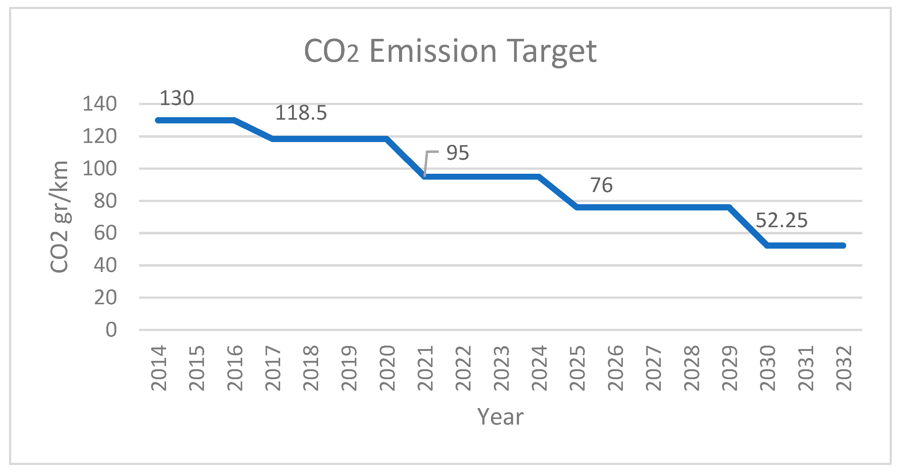
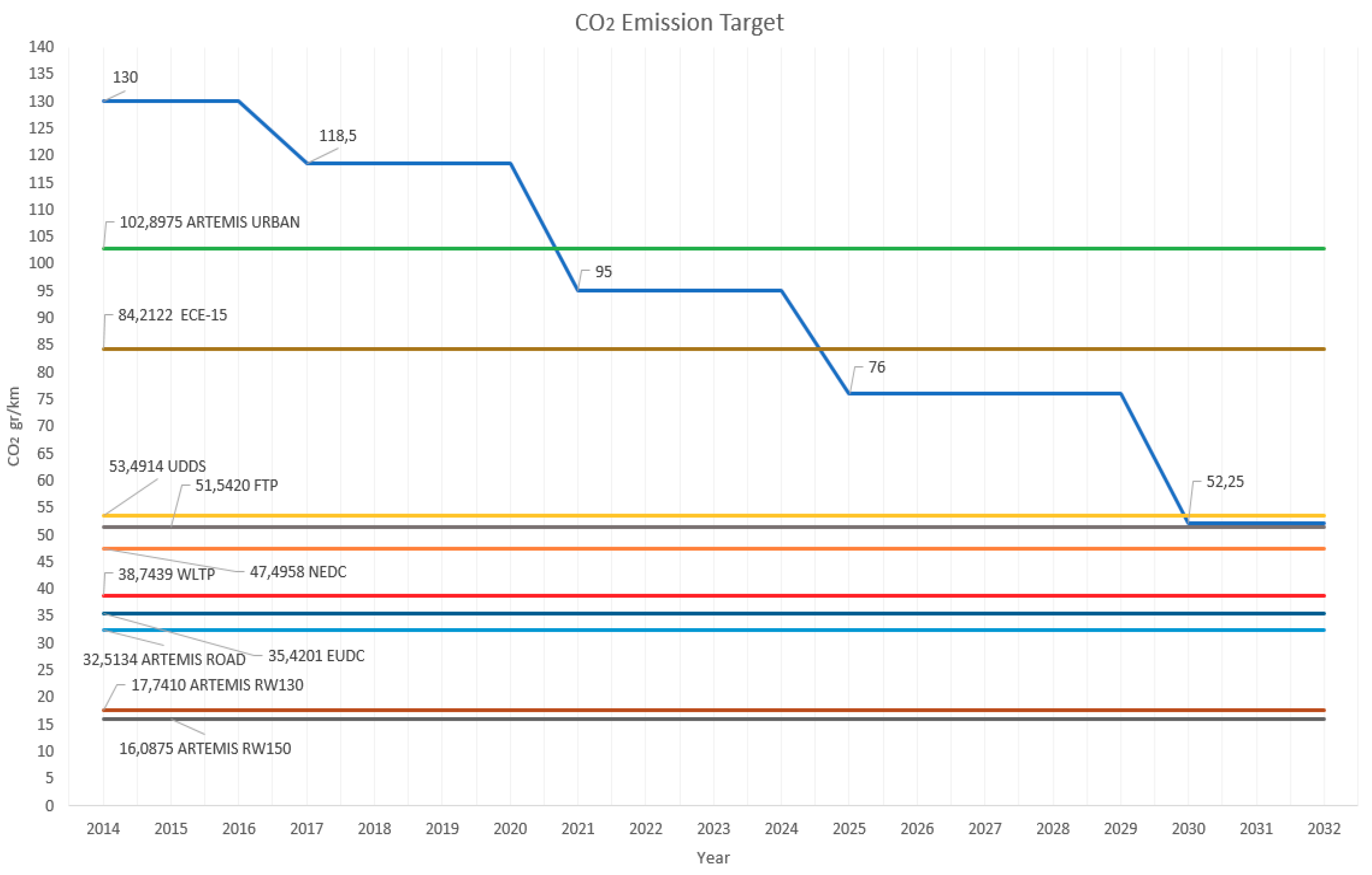
Figure 1 shows the targets′ limits of the emission of carbon dioxide from 2014 to 2030. Regarding the presented legislative limits, different types of electric vehicles are tested in to reduce pollutant and carbon dioxide (CO
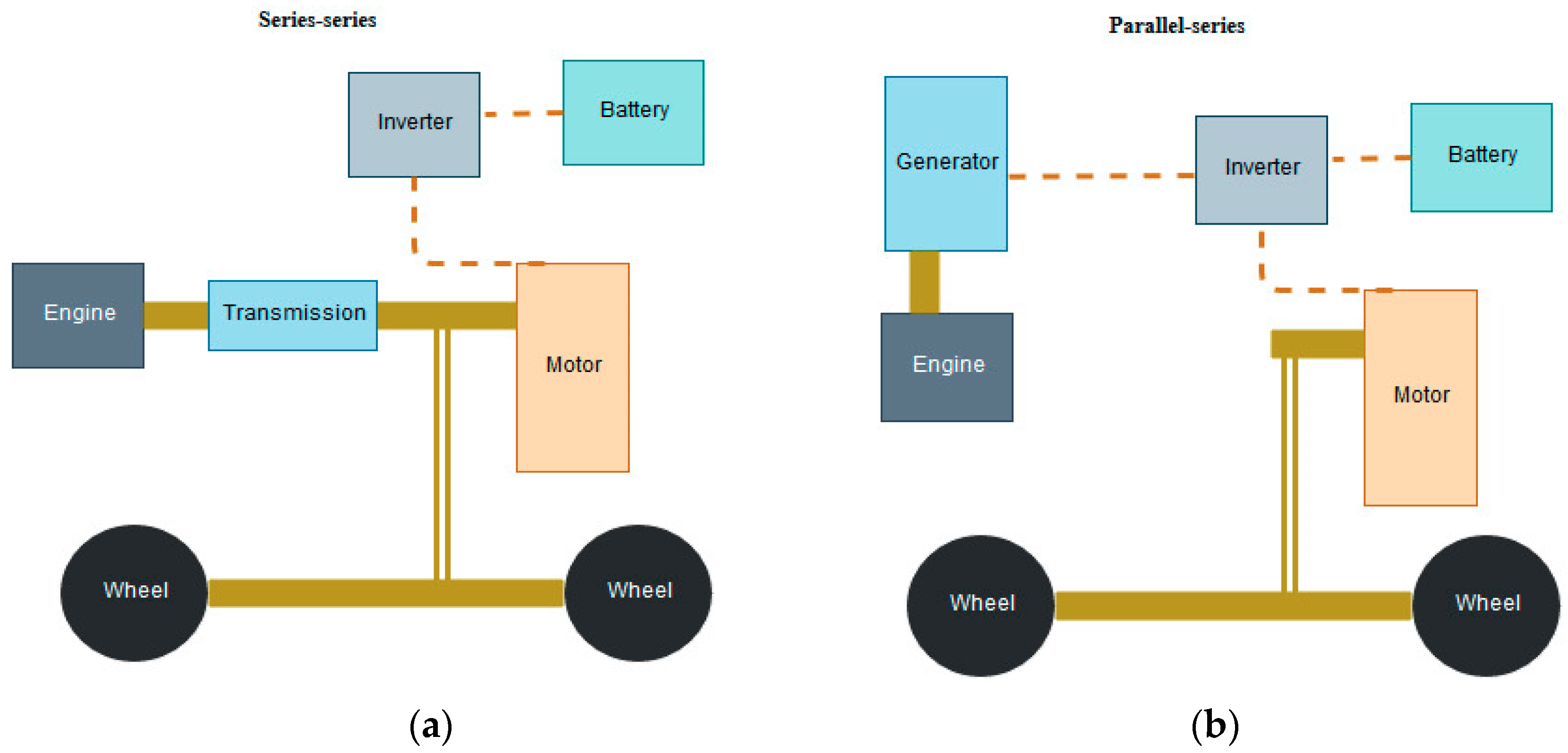
2) emissions. To respect these limits, the MHEVs needs to increase the efficiency and improve the accuracy of the measurements every year. Configurations of an MHEV that are presented by the industrial market are five: P0, P1, P2, P3, P4. Nowadays, the market prefer the configurations P0, P2, and P4. Another arrangement, mostly used in literature, classify the vehicle as series-series or series-parallel.
Figure 2 shows the difference between these classifications. When considering the standard classification of powertrain electrification technology, for the MHEVs, the P2 configuration offers an attractive solution to achieve the reduction of emissions as compared with costs. The optimization present in the vehicle includes E-charging that significantly improves the overall behavior and reduce consumption. In the vehicle study, a full dynamic is implemented that includes a longitudinal dynamic added to a vertical dynamic. The architecture schema is composed of an inverter, an engine, an electric motor, battery, and axle as shown in
Figure 2a,b. Different types of battery and electronic units have been analyzed to study the performance. The investigation of real-world measurements of a 48 V mild-hybrid electric motor with the target powertrain configuration offers impressive results, reducing costs. The real data are used to test electric motor behavior during the driving cycle. Simplifications for several model parameters are considered to reduce complexity, starting from the vehicle model containing the nonlinear system dynamics.
In the simulations of this paper, P2 configuration is presented and used. The transmission control unit, converter, and battery are integrated into the simulation to analyze the behavior of different electronic components and study the characteristics that allow for better performance. The simulation of various electronic units gives essential results for the development of new technologies in the vehicles.
E-Vehicles Model. In the vehicle stability study, two degrees of freedom vehicle model is usually applied. The longitudinal dynamics, wheel, and aerodynamic drags have been included in the vehicle model. According to [
26], the equation that describe the behavior of the vehicle are: the air resistance (6) that increase quadratically with the speed and depends on the shape of the vehicle and the air density; the rolling resistance (7) that depends on the deformation of the tire and the elastic proprieties of the road; the gradient resistance (8) that include the road with a slope; the acceleration resistance (9) is due to the changing of speed. The negative acceleration is the delay. The driving resistance is the sum of these four components (10), and the drive power (11) is the driving resistance multiplied by the speed:
where
is the air resistance;
is the air resistance at the level sea (20 °C) kg/m
3;
dependent on the shape of the vehicle drag coefficient; A is the projected face in (m
2);
is the relative speed of vehicle (m/s);
is the rolling resistance in (N);
is the mass of the vehicle in (kg);
is the mass of the load of the vehicle in (kg); g = 9.81 m/s
2 the gravitational acceleration;
is the rolling resistance coefficient; α is the angle in rad;
is the slope resistance (N);
is the mass factor (>1), which takes into account the moments of inertia of the accelerated, rotating masses in the drive train;
is the acceleration of the vehicle (m/s
2);
is the total driving resistance; and,
is the drive power. The vehicles are different from a set of parameters that is
,
,
. In this case study, the c
w is 0.28, A is 2.20,
is 1.385, and
is zero. A different set that corresponds to different vehicles and the difference from a hatchback and SUV or luxury cars depends on this set.
4. Simulation Results and Discussion
The MathWorks MATLAB/SIMULINK environment is used to verify the proposed vehicle (Equations (6)–(11)).
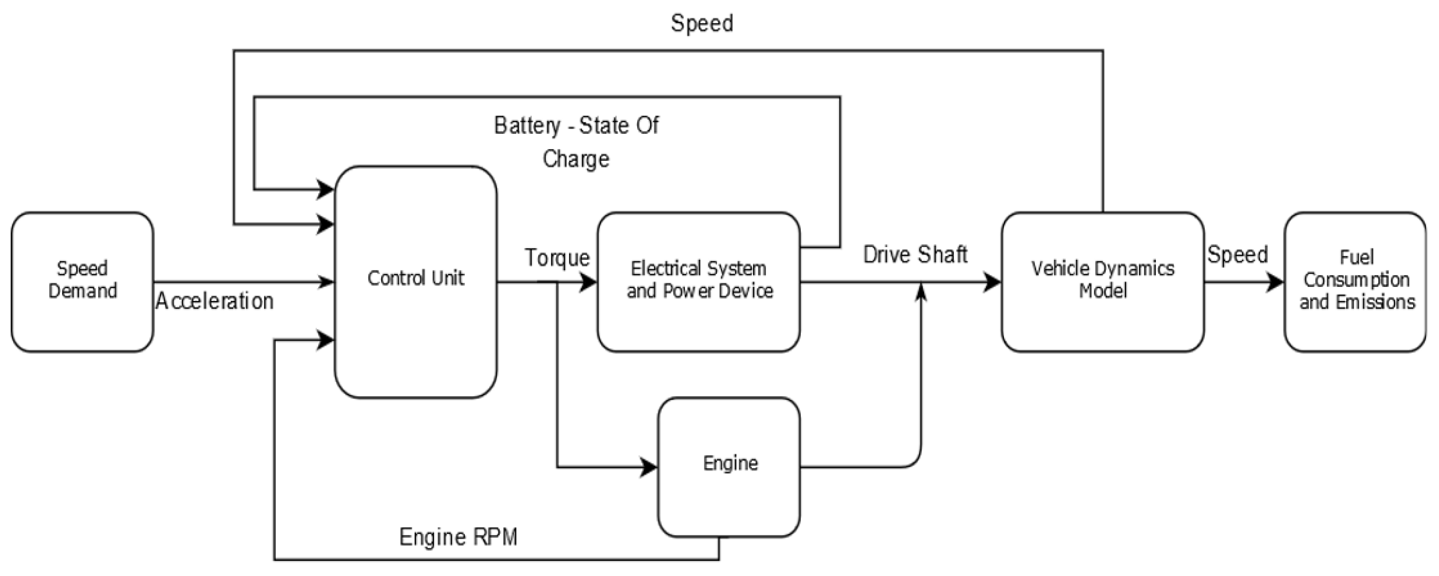
Figure 3 shows the conceptual flowchart of the functional blocks implemented on Matlab/Symulink. The simulated vehicles have been tested on different test runs.
Test runs. The tests for fuel economy are standard procedures and they are different for the country. The automotive fuel consumption is measured on a test car running with a dynamometer system. Every test simulates various driving conditions that are typical for the urban road. Europe, USA, and Australia have developed their urban cycle to determine the fuel consumption and differ in several aspects that affect it.
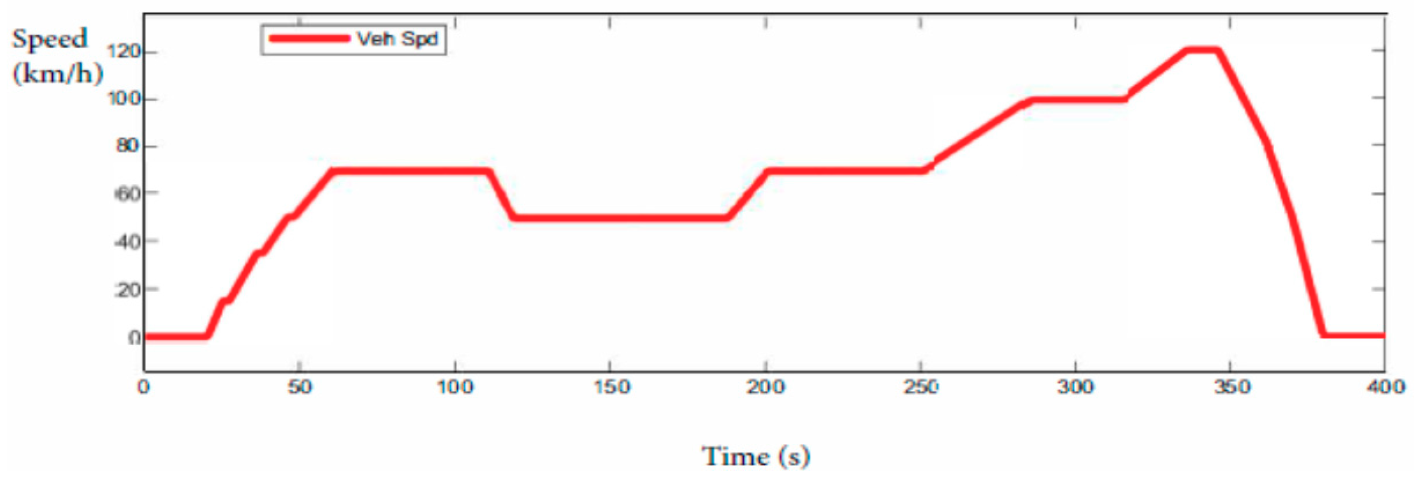
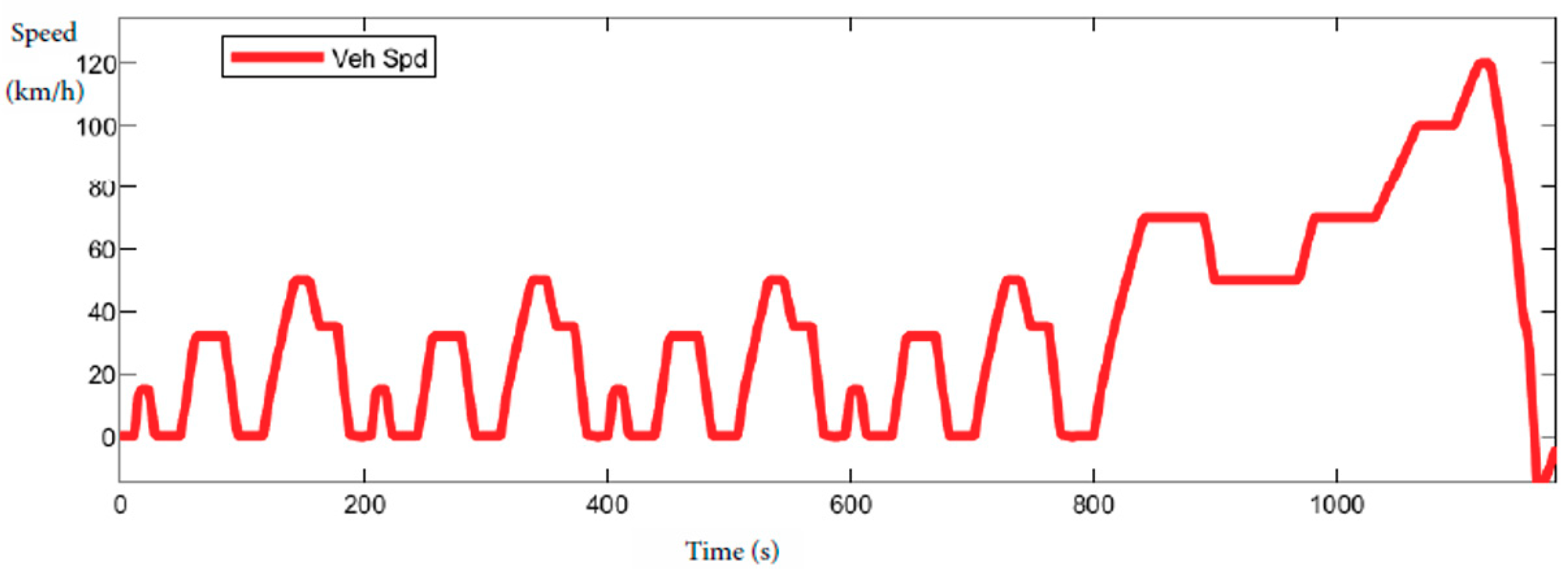
New European Driving Cycle (NEDC). The NEDC is composed of five main parts. Four-time of the ECE-15 (also called Urban Driving Cycle or UDC) repeating without interruption followed by once Extra Urban Driving Cycle (EUDC). The first part represents the city condition and low vehicle speed and low engine load define this type of cycle that reaches a maximum speed of 50 km/h. The EUDC has more aggressive high vehicle speed and the maximum speed is 120 km/h.
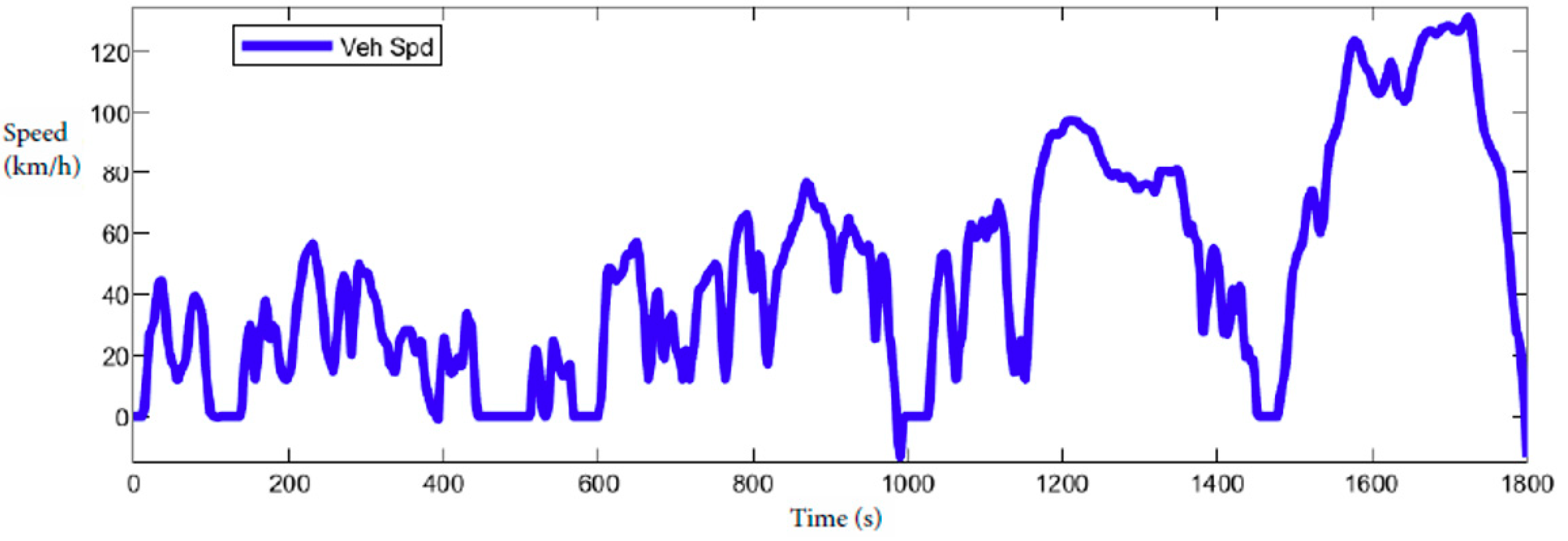
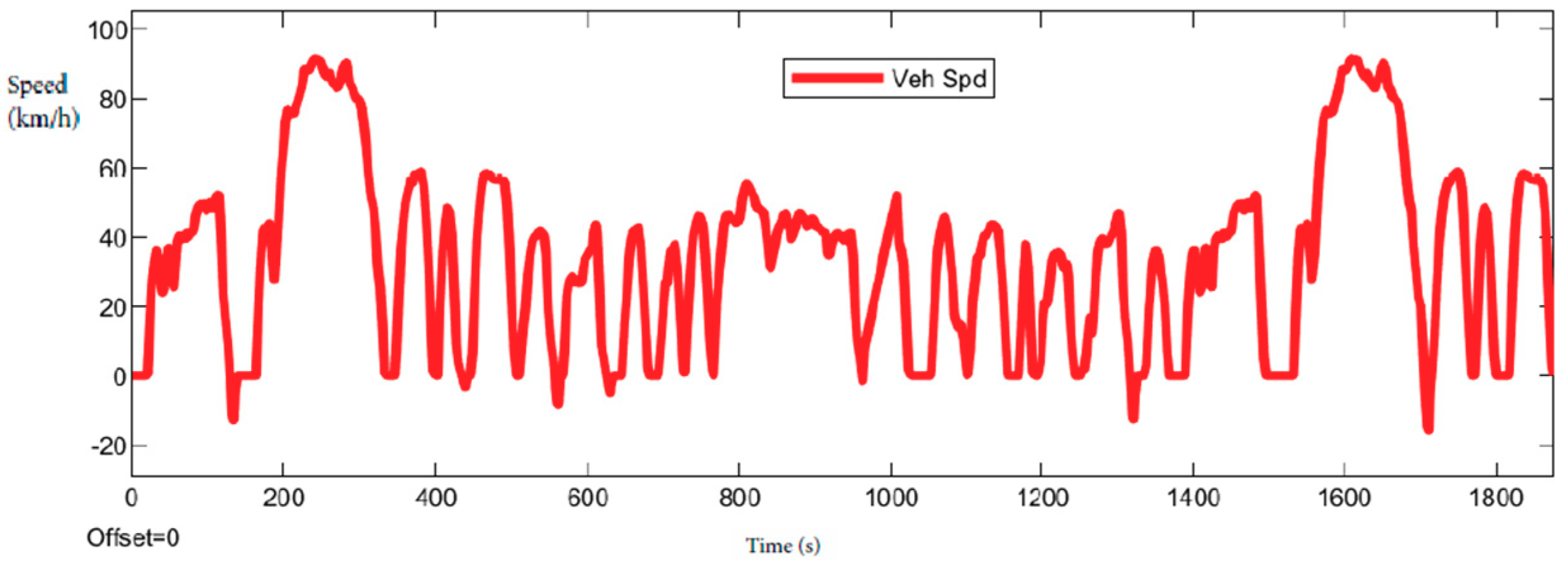
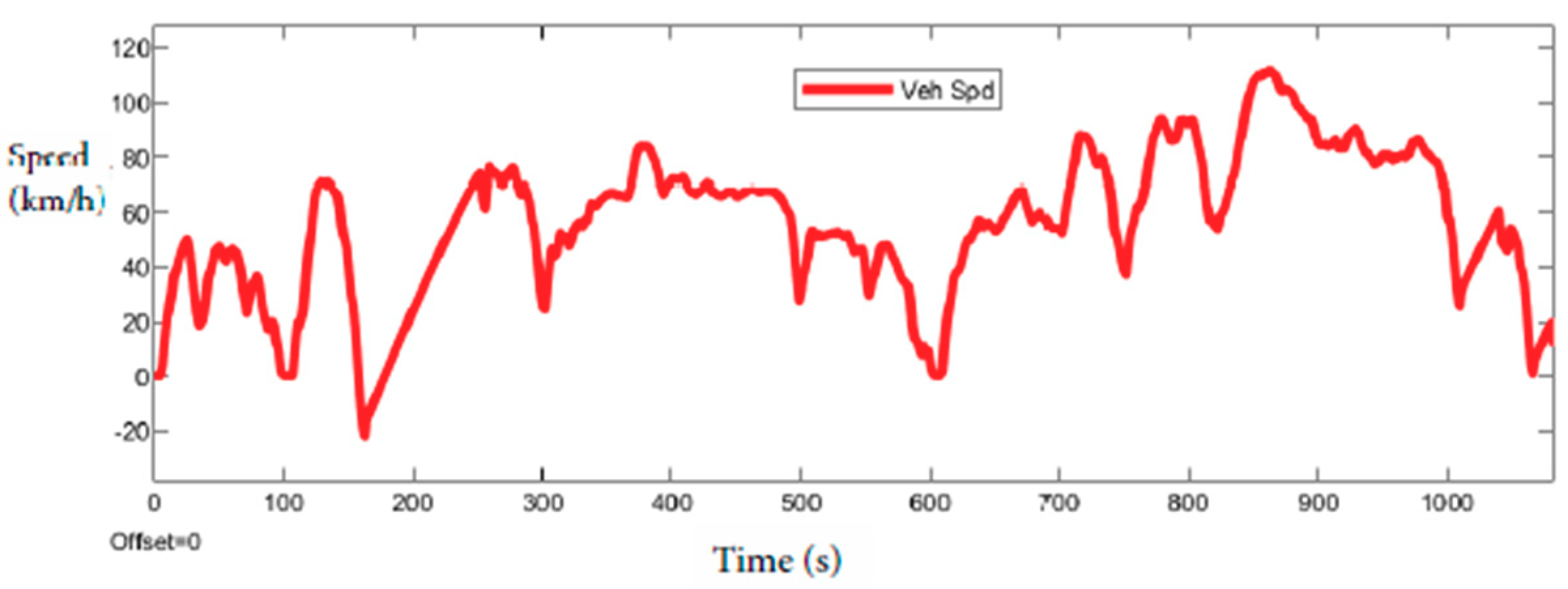
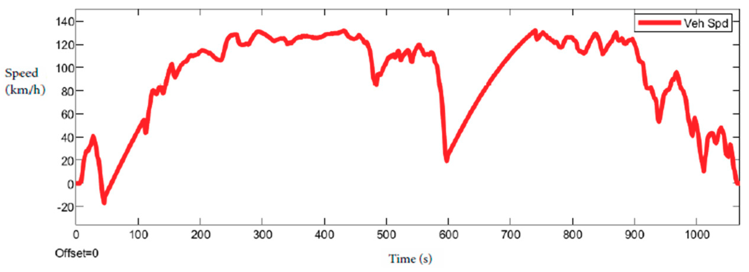
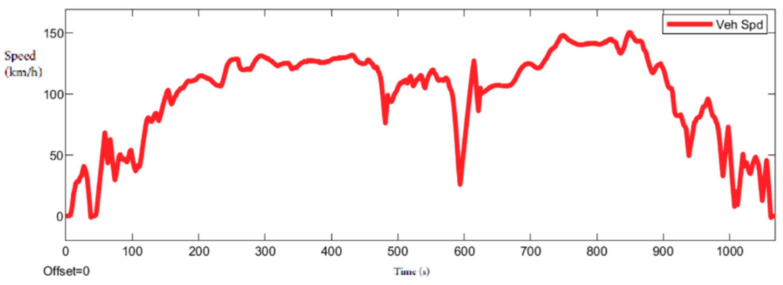
Artemis Driving Cycles. The Common Artemis Driving Cycles (CADC) are chassis dynamometer procedures that were developed within the European Artemis (Assessment and Reliability of Transport Emission Models and Inventory Systems) project, based on a statistical analysis of an extensive database of European real-world driving patterns. The cycles include four driving schedules: Urban, Rural Road, and two Motorway. The Motorway cycle has two variants with maximum speeds of 130 and 150 km/h.
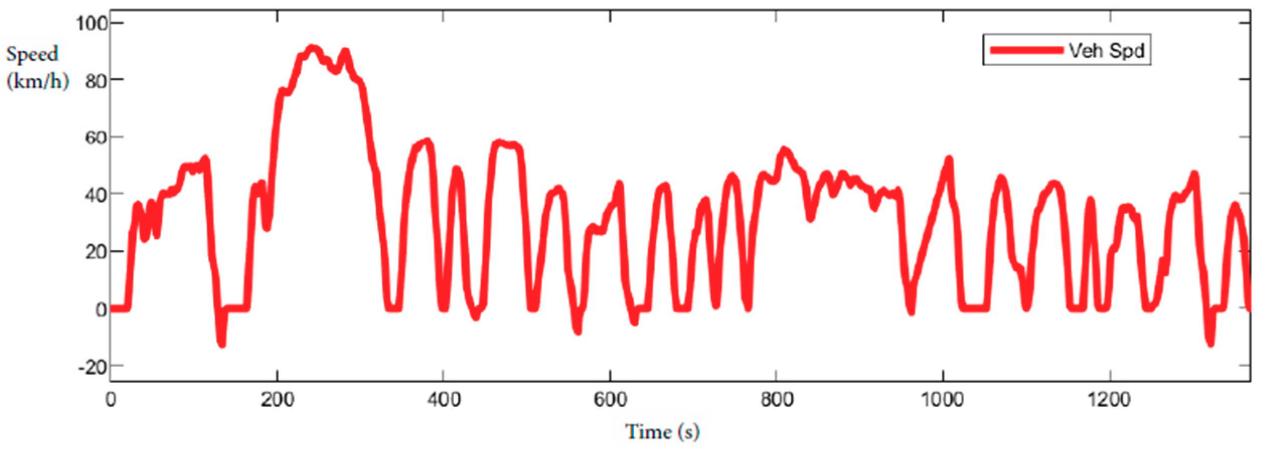
USA Test Cycle. Called SFTP US06/SC03, the SC03 Supplemental Federal Test Procedure (SFTP) represents the engine load and emissions that are associated with the use of air conditioning units in vehicles certified over the FTP-75 test cycle. The US06 Supplemental Federal Test Procedure was developed to address the shortcomings with the FTP-75 test cycle in the representation of high-speed driving and high acceleration driving behavior, speed fluctuations, and driving behavior following startup. The cycle FTP-72 (UDDS) simulates an urban route of 7.5 mi (12.07 km) with frequent stops. The maximum speed is 56.7 mph (91.25 km/h) and the average speed is 19.6 mph (31.5 km/h).
Global harmonized. The Worldwide Harmonized Light Vehicles Test Procedure (WLTP) is a global standard since 2015 for determining the level of pollutants and CO2 emissions, fuel, energy consumption, and electric range for vehicles based on real-driving data (RDE) and in laboratory test. The RDE test measures the NOx and pollutants that were emitted by cars while being driven on the road. Three different cycles are developed based on the power of the vehicle:
Class 1 – low power vehicles with PWr <= 22;
Class 2 – vehicles with 22 < PWr <= 34; and,
Class 3 – high-power vehicles with PWr > 34.
Emissions target. The Paris Agreement is an agreement within the United Nations Framework Convention on Climate Change (UNFCCC), dealing with greenhouse-gas-emissions mitigation, adaptation, and finance, signed in 2016. From 2021, phased in from 2020, the EU fleet-wide average emission target for new cars will be 95 g CO2/km. This emission level corresponds to fuel consumption of around 4.1 l/100 km of petrol or 3.6 l/100 km of diesel.
This paper is focused on presenting the interesting major cycles. The chosen cycles are NEDC, UDDS, FTP (
Table 1), ARTEMIS, shown in
Table 2, and WLTP (Class 3), shown in
Table 3.
The first results obtained while simulating the different roads show the different emission of CO
2. The circuit presented differs for consumption. This paper aims to compare the New European Driving Cycle (NEDC) with WLTP emissions and extend the analysis to the most used driving cycle in the world (
Figure 4,
Figure 5,
Figure 6,
Figure 7,
Figure 8,
Figure 9,
Figure 10,
Figure 11,
Figure 12 and
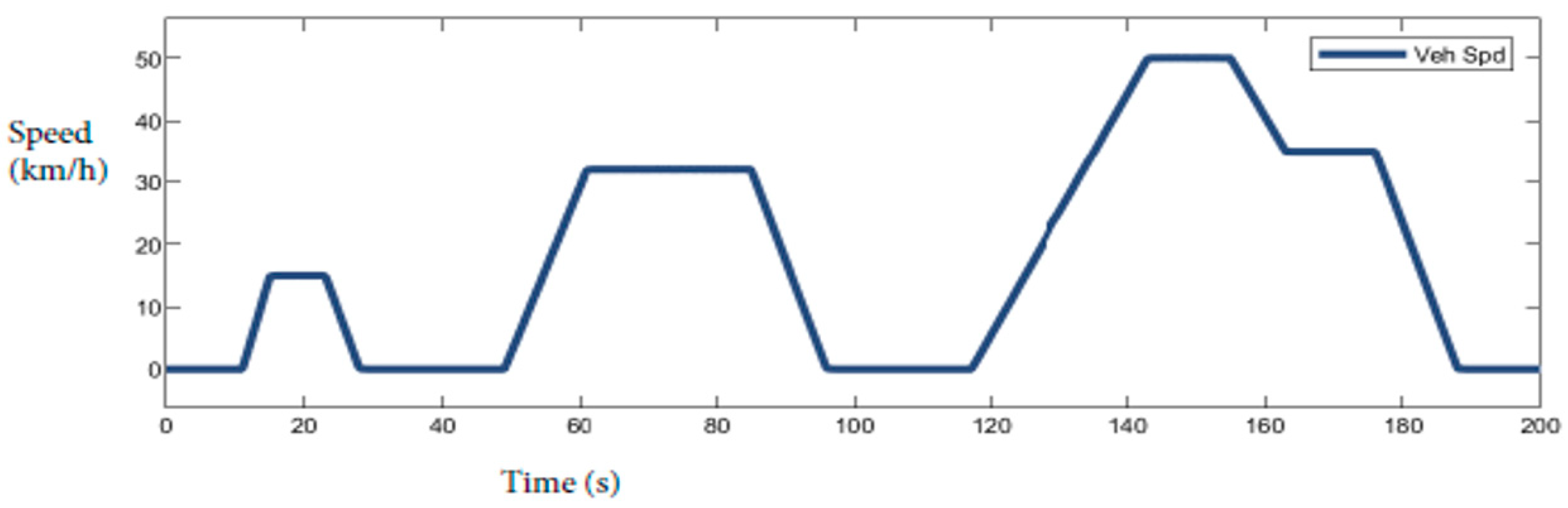
Figure 13). The NEDC is composed of two parts. The former is ECE-15 (Urban Driving Cycle), (
Figure 4) repeated four times, and the latter is EUDC (
Figure 5) once repeated. The cycle has been designed to represent typical driving conditions of busy European cities.
Figure 6 shows the complete cycle. The ECE-15 cycle is used for EU type-approval testing of emissions and fuel consumption from light-duty vehicles. The EUDC (Extra Urban Driving Cycle) segment has been added for more aggressive, high speed driving modes. The characteristic of overall driving cycle is shown in
Table 1,
Table 2 and
Table 3. When the speed is equal to zero, the emissions are considered to be zero if the engine is turned off. During the driving cycle, the emissions are equal to 2.380 g/L, the standard value measured when the speed is zero.
The ICE fuel value determines the emissions. In the graphs, the speed is negative when there are some delay. The driving profile is used for investigations of the simulation setup and to define the behavior of each component. Non-measurable quantities are estimated. From Equation (12), the total consumption
is:
where:
is the total fuel consumed,
is the distance in km, 2392 is the standard value to calculate the grams of CO
2 based on the chemical structure of CO
2.
Table 4 shows the driving cycles consumptions.
The table shows the emissions of the presented cycles. MPC is implemented in Simulink and Matlab code (see the Equations (2)–(5)). The test scenario was chosen to cover a broad operation range to investigate the performances. The MPC controller results are robust and the error is limited.
Figure 14 shows this result as compared with the emission target.


