Interval Analysis and Calculus for Interval-Valued Functions of a Single Variable. Part I: Partial Orders, gH-Derivative, Monotonicity

Abstract

We present new results in interval analysis (IA) and in the calculus for interval-valued functions of a single real variable. Starting with a recently proposed comparison index, we develop a new general setting for partial order in the (semi linear) space of compact real intervals and we apply corresponding concepts for the analysis and calculus of interval-valued functions. We adopt extensively the midpoint-radius representation of intervals in the real half-plane and show its usefulness in calculus. Concepts related to convergence and limits, continuity, gH-differentiability and monotonicity of interval-valued functions are introduced and analyzed in detail. Graphical examples and pictures accompany the presentation. A companion Part II of the paper will present additional properties (max and min points, convexity and periodicity).

1. Introduction

The motivations for this paper are two-fold: on one side we intend to offer an updated state of art about the concepts, problems and the techniques in interval analysis (IA), with a specific focus on its mathematical aspects recently addressed by research; secondly, we aim to contribute directly to the theoretical aspects of calculus in the setting of interval-valued functions of a single real variable.

We will not explicitly address the problems in interval arithmetic, in relation to the algebraic aspects of how arithmetical operations can be defined for intervals and how to solve problems such as algebraic, differential, integral equations or others when intervals are involved. An account on these topics can be found in the very extended literature on Interval Arithmetic and related fields; see, e.g., [1,2,3,4,5,6,7] (in [4] the midpoint representation is used) and the references therein.

Recently, the interest for this topic increased significantly, in particular after the new IEEE 1788–2015 Standard for Interval Arithmetic and the implementation of specific tools and classes in the C++, Julia (among others) programming languages, or in computational systems such as MATLAB, Mathematica, or in specific packages such as CORA 2016 (see [8]). The research activity in the calculus for interval-valued or set-valued functions (of one or more variables) is now very extended, particularly in connection with the more general calculus for fuzzy-valued functions (started in [9,10,11]), with applications to almost all fields of applied mathematics. One of the first contributions in the interval-valued calculus is [12] (1979); this paper remained essentially un-cited for more than 30 years and was “rediscovered” after the publication of [13,14,15]. Important contributions in this area (considering jointly the interval and fuzzy cases) are [16,17,18,19,20,21,22,23,24,25,26,27,28,29]. Other contributions are found in papers on gH-differentiability (see, e.g., [30,31,32,33,34,35,36]; see also [37,38,39]) and papers on interval and fuzzy optimization and decision making (e.g., [32,40,41,42,43,44,45,46,47,48,49,50,51,52,53,54,55,56]). A recent generalization to the multidimensional convex case is proposed in [57].

This work on the calculus for interval-valued functions is subdivided into two companion parts.

Part I presents a discussion of partial orders in the space ${\mathcal{K}}_C$ of real intervals, with properties on limits, continuity, gH-differentiability and monotonicity for functions $F:[a,b]⟶{\mathcal{K}}_C$. The basic properties of the space of real intervals are described in Section 2. Section 3 introduces several partial orders for intervals and discusses their properties in terms of the midpoint representation and in Section 4 we show the fundamental role of gH-difference in characterizing the partial orders. Section 5 introduces the concept of gH-derivative for interval valued functions and its connection with the comparison index, which is used extensively to discuss the monotonicity of interval functions in Section 6. Part I concludes with Section 7.

In Part II, using the results of part I, we present a discussion on extremal points and convexity with the use of gH-derivative for its complete analysis. A section on periodicity is also included.

2. the Space ${\mathcal{K}}_{\mathit{C}}$ of Real Intervals

We denote by ${\mathcal{K}}_C$ the family of all bounded closed intervals in $\mathbb{R}$, i.e.,

$${\mathcal{K}}_C=\left\{\left[a^{-},a^{+}\right]|a^{-},a^{+}\in \mathbb{R}\mathrm{and}{a}^{-}\le a^{+}\right\}.$$

To describe and represent basic concepts and operations for real intervals, the well-known midpoint-radius representation is very useful: for a given interval $A=\left[a^{-},a^{+}\right]$, define the midpoint $\widehat{a}$ and radius $\tilde{a}$, respectively, by

$$\widehat{a}=\frac{a^{+}+a^{-}}{2}\mathrm{and}\tilde{a}=\frac{a^{+}-a^{-}}{2},$$

so that $a^{-}=\widehat{a}-\tilde{a}$ and $a^{+}=\widehat{a}+\tilde{a}$. We denote an interval by $A=[a^{-},a^{+}]$ or, in midpoint notation, by $A=(\widehat{a};\tilde{a})$; so

$${\mathcal{K}}_C=\left\{(\widehat{a};\tilde{a})|\widehat{a},\tilde{a}\in \mathbb{R}\mathrm{and}\tilde{a}\ge 0\right\}.$$

Notation: The symbols and notation $a^{-},$ $a^{+},$ $\widehat{a},$ $\tilde{a}$, with $\tilde{a}\ge 0$, $a^{-}\le a^{+}$ (and similarly $a_i^{-},a_i^{+},{\widehat{a}}_i,{\tilde{a}}_i$,…, $z^{-},z^{+},\widehat{z},\tilde{z}$, …, $z_l^{-},z_l^{+},{\widehat{z}}_l,{\tilde{z}}_l$), using low-case characters, will refer to real intervals denoted $A,\dots Z,A_i,\dots ,Z_j\in {\mathcal{K}}_C$ in upper-case characters; when we refer to an interval $C\in {\mathcal{K}}_C$, its elements are denoted as $c^{-},$ $c^{+},$ $\widehat{c},$ $\tilde{c}$, with $\tilde{c}\ge 0$, $c^{-}\le c^{+}$ and the interval by $C=[c^{-},c^{+}]$ in extreme-point representation or, equivalently, by $C=(\widehat{c};\tilde{c})$, in midpoint notation.

Given $A=[a^{-},a^{+}],B=[b^{-},b^{+}]\in {\mathcal{K}}_C$ and $\tau \in \mathbb{R}$, we have the following classical (Minkowski-type) addition, scalar multiplication and difference:

• $A{\oplus }_{M}B=[a^{-}+b^{-},a^{+}+b^{+}]$,
• $\tau A=\{\tau a:a\in A\}=\left\{\begin{array}{cc}[\tau a^{-},\tau a^{+}],\hfill & \mathrm{if}\tau \ge 0,\hfill \\ [\tau a^{+},\tau a^{-}],\hfill & \mathrm{if}\tau \le 0\hfill \end{array}\right.$,
• $-A=(-1)A=[-a^{+},-a^{-}]$,
• $A{\ominus }_{M}B=A{\oplus }_M(-1)B=[a^{-}-b^{+},a^{+}-b^{-}]$.

Using midpoint notation, the previous operations, for $A=(\widehat{a};\tilde{a}),B=(\widehat{b};\tilde{b})$ and $\tau \in \mathbb{R}$ are:

• $A{\oplus }_{M}B=(\widehat{a}+\widehat{b};\tilde{a}+\tilde{b})$,
• $\tau A=(\tau \widehat{a};|\tau |\tilde{a})$,
• $-A=(-\widehat{a};\tilde{a})$,
• $A{\ominus }_{M}B=(\widehat{a}-\widehat{b};\tilde{a}+\tilde{b})$.

We refer to [5,6,7] for further details on interval arithmetic.

Generally, the subscript ${(·)}_M$ in the notation of Minkowski-type operations will be removed, and classical addition and subtraction will be denoted by ⊕ and ⊖, respectively, but we will insert the subscript in cases where these operations are used in combination with other operations.

We denote the generalized Hukuhara difference ($\mathrm{gH}$-difference in short) of two intervals A and B as:

$$A{\ominus }_{gH}B=C⟺\left[\begin{array}{cc}(i)\hfill & A=B{\oplus }_{M}C,\hfill \\ or\hfill & \hfill \\ (ii)\hfill & B=A{\ominus }_{M}C.\hfill \end{array}\right.$$

(1)

It is easy to show that $(i)$ and $(ii)$ are both valid if and only if C is a singleton. The $\mathrm{gH}$-difference of two intervals always exists and is equal to

$$\begin{array}{cc}\hfill A{\ominus }_{gH}B& =[min\{a^{-}-b^{-},a^{+}-b^{+}\},max\{a^{-}-b^{-},a^{+}-b^{+}\}]\hfill \\ \hfill & =(\widehat{a}-\widehat{b};|\tilde{a}-\tilde{b}|)\subseteq A{\ominus }_{M}B;\hfill \end{array}$$

the $\mathrm{gH}$-addition for intervals is defined by

$$\begin{array}{cc}\hfill A{\oplus }_{gH}B& =A{\ominus }_{gH}(-B)\hfill \\ \hfill & =[min\{a^{-}+b^{+},a^{+}+b^{-}\},max\{a^{-}+b^{+},a^{+}+b^{-}\}]\hfill \\ \hfill & =(\widehat{a}+\widehat{b};|\tilde{a}-\tilde{b}|)\subseteq A{\oplus }_{M}B.\hfill \end{array}$$

The Minkowski addition ⊕ is associative and commutative and with neutral element $\{0\}$; hereafter 0 will also denote the singleton $\{0\}$. In general, $A\ominus A\ne 0$, i.e., the opposite of A is not the inverse of A in Minkowski addition (unless $A=\{a\}$ is a singleton). A first implication of this fact is that in general, additive simplification is not valid, i.e., $(A\oplus B)\ominus B\ne A$. Instead, we always have $A{\ominus }_{gH}A=0$ and $(A{\oplus }_{M}B){\ominus }_{gH}B=A$, $\forall A,B\in {\mathcal{K}}_C$ (and other properties that will be given in the following, when needed).

If $A\in {\mathcal{K}}_C$, we will denote by $len(A)=a^{+}-a^{-}=2\widehat{a}$ the length of interval A. Remark that $\alpha A{\ominus }_M\beta A=(\alpha +\beta )A$ only if $\alpha \beta \ge 0$ (except for trivial cases) and that $A{\ominus }_{gH}B=A{\ominus }_{M}B$ or $A{\oplus }_{gH}B=A{\oplus }_{M}B$ only if A or B are singletons.

Remark 1.

The introduction of two additions ${\oplus }_M$, ${\oplus }_{gH}$ and two differences ${\ominus }_M$, ${\ominus }_{gH}$ for intervals is not motivated here as an attempt to define a “true" arithmetic in ${\mathcal{K}}_C$; for example, ${\oplus }_M$ and ${\oplus }_{gH}$ are both commutative with neutral element 0, but only ${\oplus }_M$ is associative. As we will see extensively, the four operations are each-other strongly related and their properties motivate the (appropriate) use of them in the context of interval analysis and calculus.

For two intervals $A,B\in {\mathcal{K}}_C$ the Pompeiu–Hausdorff distance $d_H:{\mathcal{K}}_C\times {\mathcal{K}}_C\to {\mathbb{R}}_{+}\cup \{0\}$ is defined by

$$d_H(A,B)=max\left\{\underset{a\in A}{max}d(a,B),\underset{b\in B}{max}d(b,A)\right\}$$

with $d(a,B)={min}_{b\in B}|a-b|$. The following properties are well known:

$$\begin{array}{cc}\hfill d_H(\tau A,\tau B)& =|\tau |d_H(A,B),\forall \tau \in \mathbb{R},\hfill \\ \hfill d_H(A\oplus C,B\oplus C)& =d_H(A,B),\hfill \\ \hfill d_H(A\oplus B,C\oplus D)& \le d_H(A,C)+d_H(B,D).\hfill \end{array}$$

It is known ([14,36]) that $d_H(A,B)=∥A{\ominus }_{gH}B∥$ where for $C\in {\mathcal{K}}_C$, the quantity $∥C∥=max\{\left|c\right|;c\in C\}=d_H(C,\left\{0\right\})$ is called the magnitude of C and an immediate property of the $\mathrm{gH}$-difference for $A,B\in {\mathcal{K}}_C$ is

$$d_H(A,B)=0⟺A{\ominus }_{gH}B=0⟺A=B.$$

(2)

It is also well known that $({\mathcal{K}}_C,d_H)$ is a complete metric space. The concepts of a convergent sequence of intervals ${(A_n)}_{n\in \mathbb{N}}$, $A_n\in {\mathcal{K}}_C$ is considered in the metric space ${\mathcal{K}}_C$, endowed with the $d_H$ distance:

Definition 1.

We say that ${lim}_{n\to \infty }{A}_n=A$ if and only if for any real $\epsilon >0$ there exists an $n_{\epsilon }\in \mathbb{N}$ such that $d_H(A_n,A)<\epsilon$ for all $n>n_{\epsilon }$.

The following equivalence is always true, as it is a trivial application of (2):

$$\underset{n\to \infty }{lim}{A}_n=A\mathrm{if}\mathrm{and}\mathrm{only}\mathrm{if}\underset{n\to \infty }{lim}\left(A_n{\ominus }_{gH}A\right)=0.$$

(3)

3. Orders for Intervals

The following partial order for intervals is well known and extensively used ($LU$ stands for Lower-Upper):

Definition 2.

Given $A=[a^{-},a^{+}]\in {\mathcal{K}}_C$, $B=[a^{-},a^{+}]\in {\mathcal{K}}_C$, we say that

(i) 

$A{⪷}_{LU}B$ if and only if $a^{-}\le b^{-}$ and $a^{+}\le b^{+}$,

(ii) 

$A{⪯}_{LU}B$ if and only if $A{⪷}_{LU}B$ and ($a^{-}<b^{-}$ or $a^{+}<b^{+}$),

(iii) 

$A{\prec }_{LU}B$ if and only if $a^{-}<b^{-}$ and $a^{+}<b^{+}$.

The corresponding reverse orders are, respectively, $A{⪸}_{LU}B⟺B{⪷}_{LU}A$, $A{⪰}_{LU}B⟺B{⪯}_{LU}A$ and $A{\succ }_{LU}B⟺B{\prec }_{LU}A$.

Using midpoint notation $A=(\widehat{a};\tilde{a})$, $B=(\widehat{b};\tilde{b})$, the partial orders $(i)$ and $(iii)$ above can be expressed as

$$(i)\left\{\begin{array}{c}\widehat{a}\le \widehat{b}\\ \tilde{b}\le \tilde{a}+(\widehat{b}-\widehat{a})\\ \tilde{b}\ge \tilde{a}-(\widehat{b}-\widehat{a})\end{array}\right.\mathrm{and}(iii)\left\{\begin{array}{c}\widehat{a}<\widehat{b}\\ \tilde{b}<\tilde{a}+(\widehat{b}-\widehat{a})\\ \tilde{b}>\tilde{a}-(\widehat{b}-\widehat{a})\end{array}\right.;$$

the partial order $(ii)$ can be expressed in terms of $(i)$ with the additional requirement that at least one of the inequalities is strict.

Proposition 1.

Let $A,B\in {\mathcal{K}}_C$ with $A=(\widehat{a};\tilde{a}),B=(\widehat{b};\tilde{b})$. We have

(i.a) 

$A{⪷}_{LU}B$ if and only if $\widehat{b}-\widehat{a}\ge \left|\tilde{b}-\tilde{a}\right|$;

(ii,a) 

$A{⪯}_{LU}B$ if and only if $\widehat{a}<\widehat{b}$ and $\widehat{b}-\widehat{a}\ge \left|\tilde{b}-\tilde{a}\right|$;

(iii,a) 

$A{\prec }_{LU}B$ if and only if $\widehat{b}-\widehat{a}>\left|\tilde{b}-\tilde{a}\right|$;

(i,b) 

$A{⪸}_{LU}B$ if and only if $\widehat{a}-\widehat{b}\ge \left|\tilde{b}-\tilde{a}\right|$;

(ii,b) 

$A{⪰}_{LU}B$ if and only if $\widehat{a}>\widehat{b}$ and $\widehat{a}-\widehat{b}\ge \left|\tilde{b}-\tilde{a}\right|$;

(iii,b) 

$A{\succ }_{LU}B$ if and only if $\widehat{a}-\widehat{b}>\left|\tilde{b}-\tilde{a}\right|$.

Proof. 

If $C=A{\ominus }_{gH}B$, then $C=[\widehat{a}-\widehat{b}-\left|\tilde{b}-\tilde{a}\right|,\widehat{a}-\widehat{b}+\left|\tilde{b}-\tilde{a}\right|]$ so that $c^{+}=\widehat{a}-\widehat{b}+\left|\tilde{b}-\tilde{a}\right|\le 0$ is equivalent to $\widehat{b}-\widehat{a}\ge \left|\tilde{b}-\tilde{a}\right|$. Analogously, $c^{-}=\widehat{a}-\widehat{b}-\left|\tilde{b}-\tilde{a}\right|\ge 0$ is equivalent to $\widehat{a}-\widehat{b}\ge \left|\tilde{b}-\tilde{a}\right|$. □

Proposition 2.

Let $A,B\in {\mathcal{K}}_C$ with $A=(\widehat{a};\tilde{a})$, $B=(\widehat{b};\tilde{b})$. We have

(i.a) 

$A{⪷}_{LU}B$ if and only if $A{\ominus }_{gH}B{⪷}_{LU}0$;

(ii.a) 

$A{⪯}_{LU}B$ if and only if $A{\ominus }_{gH}B{⪯}_{LU}0$;

(iii.a) 

$A{\prec }_{LU}B$ if and only if $A{\ominus }_{gH}B{\prec }_{LU}0$;

(i.b) 

$A{⪸}_{LU}B$ if and only if $A{\ominus }_{gH}B{⪸}_{LU}0$;

(ii.b) 

$A{⪰}_{LU}B$ if and only if $A{\ominus }_{gH}B{⪰}_{LU}0$;

(iii.b) 

$A{\succ }_{LU}B$ if and only if $A{\ominus }_{gH}B{\succ }_{LU}0$.

Proof. 

For case (i.a) we have that ${(A{\ominus }_{gH}B)}^{+}\le 0$ implies ${(A{\ominus }_{gH}B)}^{-}\le 0$ and so $A{\ominus }_{gH}B{⪷}_{LU}0$; the other cases are analogous. □

Definition 3.

Given $A,B\in {\mathcal{K}}_C$, we clearly have that

$$\begin{array}{cc}\hfill A& {\prec }_{LU}B\Rightarrow A{⪯}_{LU}B\Rightarrow A{⪷}_{LU}B\hfill \\ \hfill A& {\succ }_{LU}B\Rightarrow A{⪰}_{LU}B\Rightarrow A{⪸}_{LU}B.\hfill \end{array}$$

We say that A and B are LU-incomparable if neither $A{⪷}_{LU}B$ nor $A{⪸}_{LU}B$.

Proposition 3.

Let $A,B\in {\mathcal{K}}_C$ with $A=(\widehat{a};\tilde{a})$, $B=(\widehat{b};\tilde{b})$. The following are equivalent:

(i) 

$A$ and B are LU-incomparable;

(ii) 

$A{\ominus }_{gH}B$ is not a singleton and $0\in int(A{\ominus }_{gH}B)$;

(iii) 

$\left|\widehat{a}-\widehat{b}\right|<\left|\tilde{b}-\tilde{a}\right|$;

(iv) 

$A\subset int(B)$ or $B\subset int(A)$.

Proof. 

(i) ⟺ (ii): LU-incomparability means that neither $A{⪷}_{LU}B$ nor $A{⪸}_{LU}B$, i.e., that neither $A{\ominus }_{gH}B{⪷}_{LU}0$ nor $A{\ominus }_{gH}B{⪸}_{LU}0$ and this is equivalent with both ${\left(A{\ominus }_{gH}B\right)}^{-}<0$ and ${\left(A{\ominus }_{gH}B\right)}^{+}>0$, i.e., $0\in int(A{\ominus }_{gH}B)$.

(ii)⟺(iii): validity of (ii) means ${\left(A{\ominus }_{gH}B\right)}^{-}<0<{\left(A{\ominus }_{gH}B\right)}^{+}$ and this is equivalent to $\widehat{a}-\widehat{b}-\left|\tilde{a}-\tilde{b}\right|<0<\widehat{a}-\widehat{b}+\left|\tilde{a}-\tilde{b}\right|$ or $\left|\widehat{a}-\widehat{b}\right|<\left|\tilde{a}-\tilde{b}\right|$; so, (ii) and (iii) are equivalent.

(ii)⟺(iv): observe that $A{\ominus }_{gH}B=[min\{a^{-}-b^{-},a^{+}-b^{+}\},max\{a^{-}-b^{-},a^{+}-b^{+}\}]$; then ${\left(A{\ominus }_{gH}B\right)}^{-}<0<{\left(A{\ominus }_{gH}B\right)}^{+}$ is equivalent to $a^{-}-b^{-}<0<a^{+}-b^{+}$ or $a^{+}-b^{+}<0<a^{-}-b^{-}$. But $a^{-}-b^{-}<0<a^{+}-b^{+}$ is equivalent to $a^{-}<b^{-}$ and $a^{+}>b^{+},$ i.e., $B\subset int(A)$; and $a^{+}-b^{+}<0<a^{-}-b^{-}$ is equivalent to $a^{+}<b^{+}$ and $a^{-}>b^{-}$, i.e., $A\subset int(B)$. □

Proposition 4.

If $A,$ $B,$ $C\in {\mathcal{K}}_C$, then

(i) 

$A{⪷}_{LU}B$ if and only if $A\oplus C{⪷}_{LU}B\oplus C$;

(ii) 

If $A\oplus B{⪷}_{LU}C$ then $A{⪷}_{LU}C{\ominus }_{gH}B$;

(iii) 

If $A\oplus B{⪸}_{LU}C$ then $A{⪸}_{LU}C{\ominus }_{gH}B$

Proof. 

It is easy to check that $A{\ominus }_{gH}B=\left(A\oplus C\right){\ominus }_{gH}\left(B\oplus C\right)$ and (i) follows.

For (ii), if $A\oplus B{⪷}_{LU}C$ then ${\left((A\oplus B){\ominus }_{gH}c\right)}^{+}=max\{a^{-}+b^{-}-c^{-},a^{+}+b^{+}-c^{+}\}\le 0$ and we get $a^{-}+b^{-}\le c^{-}$ and $a^{+}+b^{+}\le c^{+}$. Then, $a^{-}\le c^{-}-b^{-}$, $a^{+}\le c^{+}-b^{+}$ and from $a^{-}\le a^{+}$ we have $a^{-}\le min\{c^{-}-b^{-},c^{+}-b^{+}\}$. On the other hand, $a^{+}\le c^{+}-b^{+}\le max\{c^{-}-b^{-},c^{+}-b^{+}\}$ and we conclude that $A{⪷}_{LU}C{\ominus }_{gH}B$.

For (iii), if $A\oplus B{⪸}_{LU}C$ then ${\left((A\oplus B){\ominus }_{gH}C\right)}^{-}=min\{a^{-}+b^{-}-c^{-},a^{+}+b^{+}-c^{+}\}\ge 0$ and we get $a^{-}+b^{-}\ge c^{-}$ and $a^{+}+b^{+}\ge c^{+}$. Then, $a^{-}\ge c^{-}-b^{-}$, $a^{+}\ge c^{+}-b^{+}$ and from $a^{+}\ge a^{-}$ we have $a^{+}\ge max\{c^{-}-b^{-},c^{+}-b^{+}\}={(C{\ominus }_{gH}B)}^{+}$; on the other hand, $a^{-}\ge c^{-}-b^{-}\ge min\{c^{-}-b^{-},c^{+}-b^{+}\}$ and we conclude that $A{⪸}_{LU}C{\ominus }_{gH}B$. □

The problem of ordering intervals has been a topic of intense research in several areas. We consider the ordering induced by the $\mathrm{gH}$-difference and the natural order on the real numbers.

Given an interval $C=\left[c^{-},c^{+}\right]=\left(\widehat{c};\tilde{c}\right)$, we define the 2-norm of C by ${∥C∥}_2=\sqrt{{\widehat{c}}^2+{\tilde{c}}^2}=\frac{\sqrt{2}}{2}\sqrt{{(c^{-})}^2+{(c^{+})}^2}$ such that ${∥C∥}_2\ge 0$, ${∥C∥}_2=0⟺C=0$, ${∥C+D∥}_2\le {∥C∥}_2+{∥D∥}_2$.

The gH-difference in midpoint notation is

$$A{\ominus }_{gH}B=\left(\widehat{\left(A{\ominus }_{gH}B\right)};\widetilde{\left(A{\ominus }_{gH}B\right)}\right)$$

where $\widehat{\left(A{\ominus }_{gH}B\right)}=\widehat{a}-\widehat{b}$ is its midpoint and $\widetilde{\left(A{\ominus }_{gH}B\right)}=|\tilde{a}-\tilde{b}|$ is its radius.

The following comparison index, based on the gH-difference and the 2-norm, has been introduced in [58,59]. We recall here the definition and the basic properties.

Definition 4.

Given two distinct intervals $A\ne B$, the gH-comparison index is defined as

$$C{I}_{gH}(A,B)=\frac{\widehat{A{\ominus }_{gH}B}}{{∥A{\ominus }_{gH}B∥}_2};$$

(4)

it has the following properties:

○

$C{I}_{gH}(A,B)\in \left[-1,1\right]$, $C{I}_{gH}(A,B)=0⟺\widehat{a}=\widehat{b}$, $C{I}_{gH}(A,B)\ge 0⟺\widehat{a}\ge \widehat{b}$,

○

$C{I}_{gH}(A,B)=-C{I}_{gH}(B,A)$, $\left|C{I}_{gH}(A,B)\right|=1⟺$($\tilde{a}=\tilde{b}$ and $\widehat{a}\ne \widehat{b}$),

○

$C{I}_{gH}(kA,kB)=\left\{\begin{array}{ccc}C{I}_{gH}(A,B)& \mathrm{if}& k>0\\ C{I}_{gH}(B,A)& \mathrm{if}& k<0,\end{array}\right.$, $C{I}_{gH}(A\oplus C,B\oplus C)=C{I}_{gH}(A,B)$.

We can write

$$C{I}_{gH}(A,B)=\frac{\widehat{a}-\widehat{b}}{\sqrt{{(\widehat{a}-\widehat{b})}^2+{(\tilde{a}-\tilde{b})}^2}}$$

and, assuming the condition $\widehat{a}\ne \widehat{b}$, we define the following gH-comparison ratio

$${\gamma }_{A,B}=\frac{\tilde{a}-\tilde{b}}{\widehat{a}-\widehat{b}}={\gamma }_{B,A}.$$

(5)

The comparison ratio ${\gamma }_{A,B}$ is very useful in the characterization of different order relations for intervals; let us consider two distinct intervals $A\ne B$ and search for (partial) order relations to decide if A is less than B, or if A is greater than B, or if A and B are incomparable.

If $\tilde{a}=\tilde{b}$ the comparison is easy as indeed, being $A\ne B$, either $\widehat{a}<\widehat{b}$ or $\widehat{a}>\widehat{b}$ and the decision can be based simply on the comparison of the midpoint values.

If $\tilde{a}\ne \tilde{b}$ and $\widehat{a}=\widehat{b}$, then A and B are incomparable with respect to any order relation; indeed, in that case, the intervals are equally centered and one of them is strictly included in the other (we can eventually have a preference for the bigger or the smaller one, but there is no simple way to quantify how much one is better or worse than the other).

The interesting and more complex case to analyze is when $\widehat{a}\ne \widehat{b}$. Consider first the comparison “A is less than B”, formally “decide if $A\prec B$ or not”. If $\widehat{a}<\widehat{b}$ and A and B do not overlap with internal points, i.e., when $a^{+}\le b^{-}$, it is reasonable to accept $A\prec B$, as no element in A is greater than any elements in B; instead, some indecision is justified if the two intervals overlap internally.

We can analyze this situation using the comparison ratio ${\gamma }_{A,B}$; we distinguish two cases, (I) $\widehat{a}<\widehat{b}$, $\tilde{a}>\tilde{b}$ and (II) $\widehat{a}<\widehat{b}$, $\tilde{a}<\tilde{b}$.

Case (I):

($\widehat{a}<\widehat{b}$ and $\tilde{a}>\tilde{b}$ so that ${\gamma }_{A,B}<0$); it is immediate to see that $a^{-}-b^{-}=(\widehat{b}-\widehat{a})({\gamma }_{A,B}-1)$. If $a^{-}\le b^{-}$, i.e., if ${\gamma }_{A,B}\le 1$, then no element in B is smaller than all elements in A. But if $a^{-}>b^{-}$, i.e., if ${\gamma }_{A,B}>1$, then elements of B exist on the left of A and the ratio $\frac{a^{-}-b^{-}}{\widehat{b}-\widehat{a}}={\gamma }_{A,B}-1>0$ measures how much elements of B are better than all elements of A, with respect to how much the central value of A is better that the central value of B. In some sense, ${\gamma }_{A,B}-1$ gives a relative measure of a possible “loss” $a^{-}-b^{-}>0$ if we chose A against B based on central values (expecting a mid-value “gain” $\widehat{b}-\widehat{a}$).

Case (II):

($\widehat{a}<\widehat{b}$ and $\tilde{a}<\tilde{b}$ so that ${\gamma }_{A,B}>0$); it is immediate to see that $a^{+}-b^{+}=(\widehat{b}-\widehat{a})(-{\gamma }_{A,B}-1)$. If $a^{+}\le b^{+}$, i.e., if ${\gamma }_{A,B}\ge -1$, then no element in A is greater than all elements in B. But if $a^{+}>b^{+}$, i.e., if ${\gamma }_{A,B}<-1$, then elements of A exist on the right of B and the ratio $\frac{a^{+}-b^{+}}{\widehat{b}-\widehat{a}}=-{\gamma }_{A,B}-1>0$ measures how many elements of A are worse than all elements of B, with respect to how much the central value of A is better than the central value of B. In some sense, $-{\gamma }_{A,B}-1$ gives a relative measure of a possible “loss” $a^{+}-b^{+}>0$ if we chose A against B based on the central values (expecting a mid-value “gain” $\widehat{b}-\widehat{a}$).

Summarizing, we can say that in accepting $A\prec B$ on the basis of the comparison $\widehat{a}<\widehat{b}$ of the midpoint values, a possibly positive (worst-case) loss appears when ${\gamma }_{A,B}>1$ or when ${\gamma }_{A,B}<-1$; we then have the following interpretation of the comparison ratio ${\gamma }_{A,B}$:

• If $\widehat{a}<\widehat{b}$ and $-1\le {\gamma }_{A,B}\le 1$, no possible worst-case loss appears in accepting $A\prec B$.
• If $\widehat{a}<\widehat{b}$ and ${\gamma }_{A,B}>1$, a possible worst-case loss in accepting $A\prec B$ appears because some values of B (on the left side) are less than all values of A; the quantity ${\gamma }_{A,B}-1>0$ gives a relative measure of the possible loss with respect to the possible midpoint gain.
• If $\widehat{a}>\widehat{b}$ and ${\gamma }_{A,B}<-1$, a possible worst-case loss in accepting $A\prec B$ appears because some values of A (on the right side) are greater than all values of B; the quantity $-1-{\gamma }_{A,B}>0$ gives a relative measure of the possible loss with respect to the midpoint gain.

The gH-comparison index ${\gamma }_{A,B}$ will be used extensively in the rest of this paper. In a similar way we can define a comparison index based on M-difference and 2-norm.

Definition 5.

Given two intervals A, B, the M-comparison index is defined as

$$C{I}_M(A,B)=\frac{\widehat{A{\ominus }_{M}B}}{{∥A{\ominus }_{M}B∥}_2}=\frac{\widehat{a}-\widehat{b}}{\sqrt{{(\widehat{a}-\widehat{b})}^2+{(\tilde{a}+\tilde{b})}^2}}$$

(6)

where $A{\ominus }_{M}B$ is the M-difference. Given two distinct intervals $A\ne B$, it has the following properties:

○

$C{I}_M(A,B)\in \left[-1,1\right]$, $C{I}_M(A,B)=0⟺\widehat{a}=\widehat{b}$, $C{I}_M(A,B)\ge 0⟺\widehat{a}\ge \widehat{b}$,

○

$C{I}_M(A,B)=-C_M(B,A)$, $\left|C{I}_M(A,B)\right|=1⟺$($\tilde{a}=\tilde{b}=0$ and $\widehat{a}\ne \widehat{b}$),

○

$C{I}_M(kA,kB)=\left\{\begin{array}{ccc}C{I}_M(A,B)& if& k>0\\ C{I}_M(B,A)& if& k<0,\end{array}\right.$, $C{I}_M(A\oplus C,B\oplus C)=C{I}_M(A,B)$.

Assuming $\widehat{a}\ne \widehat{b}$, we can define the M-comparison ratio

$${\eta }_{A,B}=\frac{\tilde{a}+\tilde{b}}{\widehat{a}-\widehat{b}}.$$

(7)

The reciprocal of the ratio ${\eta }_{A,B}$, called acceptability index

$$Acc(A\le B)=\frac{\widehat{b}-\widehat{a}}{\tilde{b}+\tilde{a}}$$

has been introduced in [60,61]: it always exists when $\tilde{a}+\tilde{b}>0$ (i.e., when at least one of A and B is a proper interval). Given two distinct intervals $A=[a^{-},a^{+}]=(\widehat{a};\tilde{a})$ and$B=[b^{-},b^{+}]=(\widehat{b};\tilde{b})$ it has the following basic properties:

(1)

if $Acc(A\le B)\ge 1$, we obtain $a^{+}\le b^{-}$ (i.e., all values of A are less than or equal to all values of B)

(2)

if $Acc(A\le B)\le -1$, we have $a^{-}\ge b^{+}$ (i.e., all values of A are greater than or equal to all values of B)

As discussed extensively in [60], if the index $Acc(A\le B)$ is positive, then it gives a measure of acceptability of the inequality $A\le B$: if $Acc(A\le B)=\alpha \in ]0,1[$ then $A\le B$ is accepted with degree $\alpha$.

The two ratios ${\gamma }_{A,B}$ and ${\eta }_{A,B}$ are not related each-other in a simple way; e.g., let’s compare $Acc(A\le B)=\frac{-1}{{\eta }_{A,B}}$ with ${\gamma }_{A,B}$ for the following intersecting intervals and in particular if $A\subset B$

1a.

$A=[3,9]=(6;3)$, $B=[4,12]=(8;4)$: $Acc(A\le B)=+\frac{2}{7}$, ${\gamma }_{A,B}=\frac{1}{2}$,

2a.

$A=[5,7]=(6;1)$, $B=[2,14]=(8;6)$: $Acc(A\le B)=+\frac{2}{7}$, ${\gamma }_{A,B}=\frac{5}{2}$,

Or if $B\subset A$

1b.

$A=[1,13]=(7;6)$, $B=[8,10]=(9;1)$: $Acc(A\le B)=+\frac{2}{7}$, ${\gamma }_{A,B}=-\frac{5}{2}$,

2b.

$A=[2,10]=(6;4)$, $B=[5,11]=(8;3)$: $Acc(A\le B)=+\frac{2}{7}$, ${\gamma }_{A,B}=-\frac{1}{2}$.

In the four cases, the acceptability index has the same value while the gH-comparison ratio has significantly different values; it is then clear that the two indices will not produce comparable results.

The three order relations ${⪷}_{LU}$, ${⪯}_{LU}$ and ${\prec }_{LU}$ in Definition 2 can be generalized in terms of the gH-comparison index as follows:

Definition 6.

Given two intervals $A=\left[a^{-},a^{+}\right]=\left(\widehat{a};\overline{a}\right)$ and $B=\left[b^{-},b^{+}\right]=(\widehat{b};\tilde{b})$ and ${\gamma }^{-}\le 0$, ${\gamma }^{+}\ge 0$ (eventually ${\gamma }^{-}=-\infty$ and/or ${\gamma }^{+}=+\infty$ ) we define the following order relation, denoted ${⪷}_{{\gamma }^{-},{\gamma }^{+}}$,

$$A{⪷}_{{\gamma }^{-},{\gamma }^{+}}B⟺\left\{\begin{array}{c}\widehat{a}\le \widehat{b}\\ \tilde{a}\ge \tilde{b}+{\gamma }^{+}\left(\widehat{a}-\widehat{b}\right)\\ \tilde{a}\le \tilde{b}+{\gamma }^{-}\left(\widehat{a}-\widehat{b}\right)\end{array}\right.$$

(8)

It is immediate to see that the relation ${⪷}_{{\gamma }^{-},{\gamma }^{+}}$ with ${\gamma }^{-}\le 0$, ${\gamma }^{+}\ge 0$ is reflexive (i.e., $A{⪷}_{{\gamma }^{-},{\gamma }^{+}}A$), antisymmetric (i.e., if $A{⪷}_{{\gamma }^{-},{\gamma }^{+}}B$ and $B{⪷}_{{\gamma }^{-},{\gamma }^{+}}A$ then $A=B$) and transitive (i.e., if $A{⪷}_{{\gamma }^{-},{\gamma }^{+}}B$ and $B{⪷}_{{\gamma }^{-},{\gamma }^{+}}C$ then $A{⪷}_{{\gamma }^{-},{\gamma }^{+}}C$). It follows that ${⪷}_{{\gamma }^{-},{\gamma }^{+}}$ is a partial order and $({\mathcal{K}}_C,{⪷}_{{\gamma }^{-},{\gamma }^{+}})$ is a lattice [59].

Definition 7.

Given two intervals $A=\left[a^{-},a^{+}\right]=\left(\widehat{a};\overline{a}\right)$ and $B=\left[b^{-},b^{+}\right]=(\widehat{b};\tilde{b})$ and ${\gamma }^{-}\le 0$, ${\gamma }^{+}\ge 0$ (eventually ${\gamma }^{-}=-\infty$ and/or ${\gamma }^{+}=+\infty$) we define the following (strict) order relation, denoted ${⪯}_{{\gamma }^{-},{\gamma }^{+}}$,

$$A{⪯}_{{\gamma }^{-},{\gamma }^{+}}B⟺\left\{\begin{array}{c}\widehat{a}<\widehat{b}\\ \tilde{a}\ge \tilde{b}+{\gamma }^{+}\left(\widehat{a}-\widehat{b}\right)\\ \tilde{a}\le \tilde{b}+{\gamma }^{-}\left(\widehat{a}-\widehat{b}\right)\end{array}\right.$$

(9)

The relation ${⪯}_{{\gamma }^{-},{\gamma }^{+}}$ with ${\gamma }^{-}\le 0$, ${\gamma }^{+}\ge 0$ is asymmetric (i.e., only one of $A{⪯}_{{\gamma }^{-},{\gamma }^{+}}B$ or $B{⪯}_{{\gamma }^{-},{\gamma }^{+}}A$ can be valid) and transitive.

Definition 8.

Given two intervals $A=\left[a^{-},a^{+}\right]=\left(\widehat{a};\overline{a}\right)$ and $B=\left[b^{-},b^{+}\right]=(\widehat{b};\tilde{b})$ and ${\gamma }^{-}\le 0$, ${\gamma }^{+}\ge 0$ (eventually ${\gamma }^{-}=-\infty$ and/or ${\gamma }^{+}=+\infty$) we define the following (strong) order relation, denoted ${\prec }_{{\gamma }^{-},{\gamma }^{+}}$,

$$A{\prec }_{{\gamma }^{-},{\gamma }^{+}}B⟺\left\{\begin{array}{c}\widehat{a}<\widehat{b}\\ \tilde{a}>\tilde{b}+{\gamma }^{+}\left(\widehat{a}-\widehat{b}\right)\\ \tilde{a}<\tilde{b}+{\gamma }^{-}\left(\widehat{a}-\widehat{b}\right)\end{array}\right.$$

(10)

The relation ${\prec }_{{\gamma }^{-},{\gamma }^{+}}$ with ${\gamma }^{-}\le 0$, ${\gamma }^{+}\ge 0$ is asymmetric and transitive.

There are specific values of ${\gamma }^{-}$ and ${\gamma }^{+}$ which make the order relation ${⪯}_{{\gamma }^{-},{\gamma }^{+}}$ equivalent to $LU$-order and other orders suggested in the literature (see [59] for details).

Proposition 5.

Let A and B be two intervals; then it holds that

(1) 

$A{⪯}_{LU}B⟺\left\{\begin{array}{c}\widehat{a}<\widehat{b}\\ \tilde{b}\le \tilde{a}+(\widehat{b}-\widehat{a})\\ \tilde{b}\ge \tilde{a}-(\widehat{b}-\widehat{a})\end{array}\right.⟺A{⪯}_{-1,1}B$, i.e., (9) with ${\gamma }^{-}=-1$ and ${\gamma }^{+}=1$,

(2) 

$A{⪯}_{C{W}_M}B⟺\widehat{a}<\widehat{b}$, $\tilde{a}\ge \tilde{b}$$⟺A{⪯}_{-\infty ,0}B$, i.e., (9) with ${\gamma }^{-}=-\infty$ and ${\gamma }^{+}=0$,

(3) 

$A{⪯}_{C{W}_m}B⟺\widehat{a}<\widehat{b}$, $\tilde{a}\le \tilde{b}⟺A{⪯}_{0,+\infty }B$, i.e., (9) with ${\gamma }^{-}=0$ and ${\gamma }^{+}=+\infty$,

(4) 

$A{⪯}_{LC}B⟺\widehat{a}<\widehat{b}$, $a^{-}\le b^{-}$$⟺\widehat{a}<\widehat{b}$, $\tilde{b}\le \tilde{a}+(\widehat{b}-\widehat{a})$$⟺A{⪯}_{-\infty ,1}B$, i.e., (9) with ${\gamma }^{-}=-\infty$ and ${\gamma }^{+}=1$,

(5) 

$A{⪯}_{UC}B⟺\widehat{a}<\widehat{b}$, $a^{+}\le b^{+}⟺\widehat{a}<\widehat{b}$, $\tilde{b}\ge \tilde{a}-(\widehat{b}-\widehat{a})⟺A{⪯}_{-1,+\infty }B$, i.e., (9) with ${\gamma }^{-}=-1$ and ${\gamma }^{+}=+\infty$.

By varying the two parameters $-\infty \le {\gamma }^{-}\le 0$, $0\le {\gamma }^{+}\le +\infty$, we obtain a continuum of partial order relations for intervals and we have the following equivalences [59]:

Proposition 6.

If A and B are two intervals then it holds that

(1) 

$A{⪷}_{LU}B⟺A{⪷}_{-1,1}B$,

(2) 

$A{⪷}_{C{W}_M}B⟺A{⪷}_{-\infty ,0}B$,

(3) 

$A{⪷}_{C{W}_m}B⟺A{⪷}_{0,+\infty }B$,

(4) 

$A{⪷}_{LC}B⟺A{⪷}_{-\infty ,1}B$,

(5) 

$A{⪷}_{UC}B⟺A{⪷}_{-1,+\infty }B$.

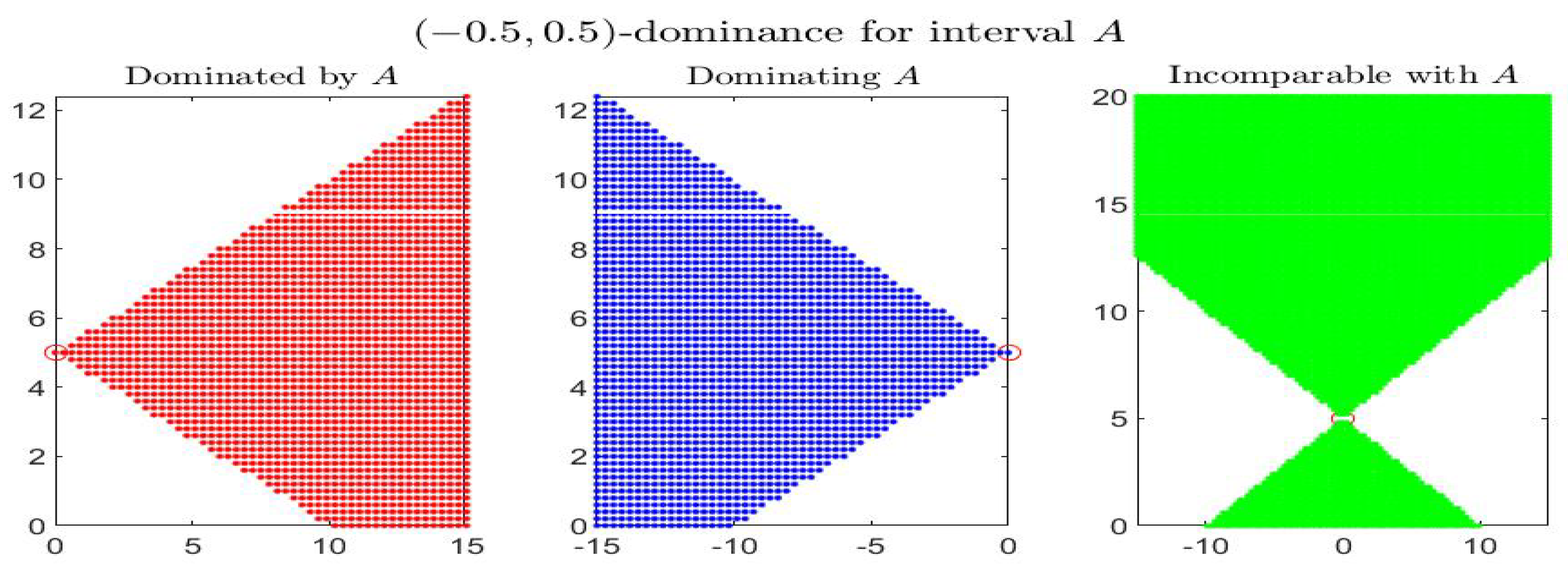
Remark 2.

To have $A{⪷}_{{\gamma }^{-}{\gamma }^{+}}B$ we need $\widehat{a}\le \widehat{b}$ and $\tilde{b}+{\gamma }^{+}\left(\widehat{a}-\widehat{b}\right)$ $\le \tilde{a}\le \tilde{b}+{\gamma }^{-}\left(\widehat{a}-\widehat{b}\right)$. It follows that for the order relation ${⪷}_{{\gamma }^{-},{\gamma }^{+}}$ with ${\gamma }^{-}\le 0,{\gamma }^{+}\ge 0$ in ${\mathcal{K}}_C$, we have the equivalence

$$\begin{array}{c}\hfill A{⪷}_{{\gamma }^{-},{\gamma }^{+}}B⟺(A{⪯}_{{\gamma }^{-},{\gamma }^{+}}BorA=B).\end{array}$$

(11)

Definition 9.

For a given interval $A=(\widehat{a};\tilde{a})$, we define the following sets of intervals X which are

(a) 

$({⪷}_{{\gamma }^{-},{\gamma }^{+}})$-dominated by A:

$${\mathbb{D}}_{<}(A;{\gamma }^{-},{\gamma }^{+})=\{X\in {\mathcal{K}}_C|A{⪷}_{{\gamma }^{-},{\gamma }^{+}}X\},$$

(12)

(b) 

$({⪷}_{{\gamma }^{-},{\gamma }^{+}})$-dominating A:

$${\mathbb{D}}_{>}(A;{\gamma }^{-},{\gamma }^{+})=\{X\in {\mathcal{K}}_C|X{⪷}_{{\gamma }^{-},{\gamma }^{+}}A\},$$

(13)

(c) 

$({⪷}_{{\gamma }^{-},{\gamma }^{+}})$-incomparable with A:

$$\mathbb{I}(A;{\gamma }^{-},{\gamma }^{+})=\{X\in {\mathcal{K}}_C|X\notin {\mathbb{D}}_{<}(A;{\gamma }^{-},{\gamma }^{+}),X\notin {\mathbb{D}}_{>}(A;{\gamma }^{-},{\gamma }^{+})\}.$$

(14)

Proposition 7.

For any $-\infty <{\gamma }^{-}<0$, $0<{\gamma }^{+}<+\infty$ and any intervals $A,B\in {\mathcal{K}}_C$, we have

a.

$A{⪷}_{{\gamma }^{-},{\gamma }^{+}}B$ if and only if ${\mathbb{D}}_{<}(B;{\gamma }^{-},{\gamma }^{+})\subseteq {\mathbb{D}}_{<}(A;{\gamma }^{-},{\gamma }^{+})$;

b.

$A=B$ if and only if ${\mathbb{D}}_{<}(A;{\gamma }^{-},{\gamma }^{+})={\mathbb{D}}_{<}(B;{\gamma }^{-},{\gamma }^{+})$;

c.

$\varnothing ={\mathbb{D}}_{<}(A;{\gamma }^{-},{\gamma }^{+})\bigcap \mathbb{I}(A;{\gamma }^{-},{\gamma }^{+})={\mathbb{D}}_{>}(A;{\gamma }^{-},{\gamma }^{+})\bigcap \mathbb{I}(A;{\gamma }^{-},{\gamma }^{+})$;

d.

$\{A\}={\mathbb{D}}_{<}(A;{\gamma }^{-},{\gamma }^{+})\bigcap {\mathbb{D}}_{>}(A;{\gamma }^{-},{\gamma }^{+})$;

e.

${\mathcal{K}}_C=\mathbb{I}(A;{\gamma }^{-},{\gamma }^{+})\bigcup$${\mathbb{D}}_{<}(A;{\gamma }^{-},{\gamma }^{+})\bigcup {\mathbb{D}}_{>}(A;{\gamma }^{-},{\gamma }^{+})$.

Proof. 

The proof of all the properties can be easily obtained by direct manipulation of involved definitions; we omit the details. □

Consider the following example: the four figures show, for the given interval $A=(0;5)=[-5,5]$, the corresponding set of dominated, dominating and incomparable intervals, respectively the sets ${\mathbb{D}}_{<}(A;{\gamma }^{-},{\gamma }^{+})$ (red colored pictures), ${\mathbb{D}}_{>}(A;{\gamma }^{-},{\gamma }^{+})$ (blue-colored regions) and $\mathbb{I}(A;{\gamma }^{-},{\gamma }^{+})$ (in green color), for partial orders (${⪷}_{{\gamma }^{-},{\gamma }^{+}}$) with four different pairs $({\gamma }^{-},{\gamma }^{+})$. In particular it is shown: $(-1,1)$-dominance (i.e., $LU$-dominance) in Figure 1, $(-0.5,0.5)$-dominance in Figure 2, $(-1,2)$-dominance in Figure 3 and $(-1,0.5)$-dominance in Figure 4. All the figures consider intervals $X=(\widehat{x};\tilde{x})$ in the range $\widehat{x}\in [-15,15]$ and $\tilde{x}\in [0,20]$.

By inspecting the four figures, we see that with respect to the $LU$-order (Figure 1, with ${\gamma }^{+}=-{\gamma }^{-}=1$) or an order with ${\gamma }^{-}+{\gamma }^{+}=0$ (Figure 2, with ${\gamma }^{+}=-{\gamma }^{-}=0.5$), the set of incomparable intervals is symmetric with respect to the vertical line $\widehat{x}=\widehat{a}$; when ${\gamma }^{-}+{\gamma }^{+}>0$ (Figure 3) the right part of the incomparable region, determined by an increase of ${\gamma }^{+}>1$, tends to become more vertical and reduces in favor of the dominated region (red colored) and the dominating region (blue-colored). The opposite effect appears if ${\gamma }^{+}<1$ decreases (Figure 4).

The lattice structure of ${\mathcal{K}}_C$, endowed with the partial order ${⪷}_{{\gamma }^{-},{\gamma }^{+}}$, can be further analyzed by considering the basic concepts of least upper bound (lub or sup) and greatest lower bound (glb or inf). For two intervals $A,B\in {\mathcal{K}}_C$, a (common) upper bound is an interval $Z\in {\mathcal{K}}_C$ such that $A{⪷}_{{\gamma }^{-},{\gamma }^{+}}Z$ and $B{⪷}_{{\gamma }^{-},{\gamma }^{+}}Z$. A (common) lower bound is an interval $Z\in {\mathcal{K}}_C$ such that $Z{⪷}_{{\gamma }^{-},{\gamma }^{+}}A$ and $Z{⪷}_{{\gamma }^{-},{\gamma }^{+}}B$.

The least upper bound for $A,B$, denoted $lub(A,B)$ or $sup(A,B)$, is a common upper bound Z such that every other upper bound $Z^{\prime }$ is such that $Z{⪷}_{{\gamma }^{-},{\gamma }^{+}}{Z}^{\prime }$; analogously, the greatest lower bound for $A,B$, denoted $glb(A,B)$ or $inf(A,B)$, is a common lower bound Z such that every other lower bound $Z^{\prime }$ is such that $Z^{\prime }{⪷}_{{\gamma }^{-},{\gamma }^{+}}Z$. It is immediate to see that $inf(A,B)$ and $sup(A,B)$ always exist (and are unique) for any $A,B\in {\mathcal{K}}_C$ (see [59] for details).

If $\mathbb{S}\subset {\mathcal{K}}_C$ is any subset of intervals, we say that $\mathbb{S}$ is bounded from below (lower bounded) with respect to ${⪷}_{{\gamma }^{-},{\gamma }^{+}}$ if and only if there exists $L\in {\mathcal{K}}_C$ such that $L{⪷}_{{\gamma }^{-},{\gamma }^{+}}X$ for all $X\in \mathbb{S}$ and we say that $\mathbb{S}$ is bounded from above (upper bounded) with respect to ${⪷}_{{\gamma }^{-},{\gamma }^{+}}$ if and only if there exists $U\in {\mathcal{K}}_C$ such that $X{⪷}_{{\gamma }^{-},{\gamma }^{+}}U$ for all $X\in \mathbb{S}$. If $\mathbb{S}\subset {\mathcal{K}}_C$ is both lower and upper bounded, we say it is bounded.

Every bounded subset of ${\mathcal{K}}_C$ admits inf and sup.

Proposition 8.

Consider a partial order ${⪷}_{{\gamma }^{-},{\gamma }^{+}}$ on ${\mathcal{K}}_C$ and let $\mathbb{S}\subset {\mathcal{K}}_C$ be any nonempty bounded subset of intervals. Then, there exist both ${inf}_{{\gamma }^{-},{\gamma }^{+}}(\mathbb{S}),{sup}_{{\gamma }^{-},{\gamma }^{+}}(\mathbb{S})\in {\mathcal{K}}_C$ such that for all $X\in \mathbb{S}$

$$inf(\mathbb{S}){⪷}_{{\gamma }^{-},{\gamma }^{+}}X{⪷}_{{\gamma }^{-},{\gamma }^{+}}sup(\mathbb{S}).$$

(15)

We also have, for all $A\in {\mathcal{K}}_C$,

$$A=inf({\mathbb{D}}_{<}(A;{\gamma }^{-},{\gamma }^{+}))\mathit{and}A=sup({\mathbb{D}}_{>}(A;{\gamma }^{-},{\gamma }^{+})).$$

(16)

Proof. 

We will prove only Equation (15) by a constructive procedure; the proof of equations in (16) is immediate. Let $L=(\widehat{l};\tilde{l})\in {\mathcal{K}}_C$ be any lower bound and $U=(\widehat{u};\tilde{u})\in {\mathcal{K}}_C$ any upper bound for $\mathbb{S}$ and consider the four lines, in the half-plane $(\widehat{x};\tilde{x})$, with equations

$$\tilde{x}=\tilde{l}+{\gamma }^{+}\left(\widehat{x}-\widehat{l}\right)\mathrm{and}\tilde{x}=\tilde{l}+{\gamma }^{-}\left(\widehat{x}-\widehat{l}\right)(\mathrm{through}\mathrm{point}L),$$

$$\tilde{x}=\tilde{u}+{\gamma }^{+}\left(\widehat{x}-\widehat{u}\right)\mathrm{and}\tilde{x}=\tilde{u}+{\gamma }^{-}\left(\widehat{x}-\widehat{u}\right)(\mathrm{through}\mathrm{point}U).$$

They intersect the vertical axis $(\widehat{x}=0)$ with intercepts, respectively, $q_L^{+}=\tilde{l}-{\gamma }^{+}\widehat{l}$, $q_L^{-}=\tilde{l}-{\gamma }^{-}\widehat{l}$ and $q_U^{+}=\tilde{u}-{\gamma }^{+}\widehat{u}$, $q_U^{-}=\tilde{u}-{\gamma }^{-}\widehat{u}$. Considering an arbitrary element $S=(\widehat{s};\tilde{s})\in \mathbb{S}$, the two lines trough S with angular coefficients ${\gamma }^{+}$ and ${\gamma }^{-}$, with equations $\tilde{x}=\tilde{s}+{\gamma }^{+}\left(\widehat{x}-\widehat{s}\right)$ and $\tilde{x}=\tilde{s}+{\gamma }^{-}\left(\widehat{x}-\widehat{s}\right)$, respectively, have intercepts $q_S^{+}=\tilde{s}-{\gamma }^{+}\widehat{s}$, $q_S^{-}=\tilde{s}-{\gamma }^{-}\widehat{s}$ and their sets $Q^{+}=\left\{q_S^{+}|S\in \mathbb{S}\right\}$ and $Q^{-}=\left\{q_S^{-}|S\in \mathbb{S}\right\}$ are both bounded with $q_U^{+}\le q_S^{+}\le q_L^{+}$ and $q_L^{-}\le q_S^{-}\le q_U^{-}$ for all $S\in \mathbb{S}$. Consequently, there exist the four real numbers $q_{inf}^{+}=inf{Q}^{+}$, $q_{sup}^{+}=sup{Q}^{+}$, $q_{inf}^{-}=inf{Q}^{-}$, $q_{sup}^{-}=sup{Q}^{-}$ with $q_{inf}^{+}\le q_{sup}^{+}$ and $q_{inf}^{-}\le q_{sup}^{-}$. Finally, the intersection point of the two lines $\tilde{x}=q_{sup}^{+}+{\gamma }^{+}\widehat{x}$ and $\tilde{x}=q_{inf}^{-}+{\gamma }^{-}\widehat{x}$ corresponds to the interval $inf\mathbb{S}\in {\mathcal{K}}_C$; analogously, the intersection point of the two lines $\tilde{x}=q_{inf}^{+}+{\gamma }^{+}\widehat{x}$ and $\tilde{x}=q_{sup}^{-}+{\gamma }^{-}\widehat{x}$ corresponds to the interval $sup\mathbb{S}\in {\mathcal{K}}_C$. More precisely, we have

$$inf\mathbb{S}=\left({\displaystyle \frac{q_{sup}^{+}-q_{inf}^{-}}{{\gamma }^{-}-{\gamma }^{+}}};{\displaystyle \frac{{\gamma }^{-}{q}_{sup}^{+}-{\gamma }^{+}{q}_{inf}^{-}}{{\gamma }^{-}-{\gamma }^{+}}}\right)$$

and

$$sup\mathbb{S}=\left({\displaystyle \frac{q_{inf}^{+}-q_{sup}^{-}}{{\gamma }^{-}-{\gamma }^{+}}};{\displaystyle \frac{{\gamma }^{-}{q}_{inf}^{+}-{\gamma }^{+}{q}_{sup}^{-}}{{\gamma }^{-}-{\gamma }^{+}}}\right)$$

This completes the proof. □

If, for a nonempty bounded subset $\mathbb{S}\subset {\mathcal{K}}_C$ we have that $inf(\mathbb{S})$ or $sup(\mathbb{S})$ are elements of $\mathbb{S}$, then there exist the intervals $min(\mathbb{S})$ or, respectively, $max(\mathbb{S})$.

Interesting bounded subsets in ${\mathcal{K}}_C$ are the “segment” with extremes $A,B\in {\mathcal{K}}_C$ and the “interval” with extremes $A,B\in {\mathcal{K}}_C$, defined, respectively, by

$$\lambda (A,B)=\left\{X_{\lambda }|X_{\lambda }=(1-\lambda )A+\lambda B,\lambda \in [0,1]\right\},$$

(17)

and, assuming $A{⪷}_{{\gamma }^{-},{\gamma }^{+}}B$ (here, the dominance is essential),

$$[A,B]=\left\{X\in {\mathcal{K}}_C|A{⪷}_{{\gamma }^{-},{\gamma }^{+}}X{⪷}_{{\gamma }^{-},{\gamma }^{+}}B\right\}.$$

(18)

If $\mathbb{S}$ is a bounded subset of ${\mathcal{K}}_C$, we clearly have $\mathbb{S}\subseteq [inf(\mathbb{S}),sup(\mathbb{S})]$, with equality if and only if $\mathbb{S}=[A,B]$ with $A=inf(\mathbb{S}),B=sup(\mathbb{S})$.

We conclude this section with an interesting property.

Proposition 9.

For a given partial order ${⪷}_{{\gamma }^{-},{\gamma }^{+}}$ with ${\gamma }^{-}\le 0$, ${\gamma }^{+}\ge 0$, consider the partial order ${⪷}_{-{\gamma }^{+},-{\gamma }^{-}}$; then, for all $A,B$,

$$A{⪷}_{{\gamma }^{-},{\gamma }^{+}}B⟺(-B){⪷}_{-{\gamma }^{+},-{\gamma }^{-}}(-A),$$

(19)

where $-A$ and $-B$ are the opposite intervals of A and B.

Proof. 

Starting with inequalities (8) that define $A{⪷}_{{\gamma }^{-},{\gamma }^{+}}B$ and recalling that $-A=(-\widehat{a};\tilde{a})$ the conclusion follows after a few simple algebraic manipulations. □

In particular, if ${\gamma }^{-}+{\gamma }^{+}=0$, i.e., ${\gamma }^{+}=-{\gamma }^{-}=\gamma \ge 0$ so that $({⪷}_{{\gamma }^{-},{\gamma }^{+}})\equiv ({⪷}_{-{\gamma }^{+},-{\gamma }^{-}})\equiv ({⪷}_{\gamma })$, we have that for any bounded subset $\mathbb{S}\subset {\mathcal{K}}_C$,

$$inf(\mathbb{S})=-sup(-\mathbb{S})$$

(20)

where the (bounded) subset $-\mathbb{S}\subset {\mathcal{K}}_C$ is defined by

$$-\mathbb{S}=\left\{-X|X\in \mathbb{S}\right\}.$$

(21)

4. Orders in ${\mathcal{K}}_{\mathit{C}}$ and Gh-Difference

In this section, we express a partial order ${⪷}_{{\gamma }^{-},{\gamma }^{+}}$ in terms of the gH-difference $A{\ominus }_{gH}B=(\widehat{a}-\widehat{b};|\tilde{a}-\tilde{b}|)$.

Recall that from

$$A{⪷}_{{\gamma }^{-},{\gamma }^{+}}B⟺(A{⪯}_{{\gamma }^{-},{\gamma }^{+}}B\mathrm{or}A=B),$$

we can write

$$A{⪷}_{{\gamma }^{-},{\gamma }^{+}}B⟺\left\{\begin{array}{c}\widehat{a}\le \widehat{b}\\ \tilde{a}\ge \tilde{b}+{\gamma }^{+}\left(\widehat{a}-\widehat{b}\right)\\ \tilde{a}\le \tilde{b}+{\gamma }^{-}\left(\widehat{a}-\widehat{b}\right)\end{array}\right.$$

(22)

and, for the reverse order,

$$A{⪸}_{{\gamma }^{-},{\gamma }^{+}}B⟺\left\{\begin{array}{c}\widehat{a}\ge \widehat{b}\\ \tilde{a}\le \tilde{b}+{\gamma }^{+}\left(\widehat{a}-\widehat{b}\right)\\ \tilde{a}\ge \tilde{b}+{\gamma }^{-}\left(\widehat{a}-\widehat{b}\right).\end{array}\right.$$

(23)

Remark 3.

One may think that condition $\widehat{a}\le \widehat{b}$ is redundant in (22); indeed, if ${\gamma }^{-}<0$ or ${\gamma }^{+}>0$, it is implied by the second and third conditions. But if $\tilde{a}=\tilde{b}=0$ and ${\gamma }^{-}={\gamma }^{+}=0$, the order reduces to the standard order for real numbers while the second and the third conditions reduce to inequalities $0\ge 0$ and $0\le 0$. For this reason we will always include condition $\widehat{a}\le \widehat{b}$ in (22). If ${\gamma }^{-}<0$ or ${\gamma }^{+}>0$ and the second and third conditions are both satisfied with equality, then $A=B$ and vice versa.

We have the following results.

Lemma 1.

Let $A,B\in {\mathcal{K}}_C$ and consider the lattice $({\mathcal{K}}_C,{⪷}_{{\gamma }^{-},{\gamma }^{+}})$ with ${\gamma }^{-}<0$ and ${\gamma }^{+}>0$; then

(1a) $A{⪷}_{{\gamma }^{-},{\gamma }^{+}}B$⟹$A{\ominus }_{gH}B{⪷}_{{\gamma }^{-},{\gamma }^{+}}0$ (in the right part of implication, ${\gamma }^{+}$ is not involved);

(1b) $A{⪷}_{{\gamma }^{-},{\gamma }^{+}}B$⟹ $0{⪷}_{{\gamma }^{-},{\gamma }^{+}}B{\ominus }_{gH}A$ (in the right part of implication, ${\gamma }^{-}$ is not involved);

(2) $A{⪷}_{{\gamma }^{-},{\gamma }^{+}}B⟺\left(A{\ominus }_{gH}B{⪷}_{{\gamma }^{-},{\gamma }^{+}}0\mathrm{and}B{\ominus }_{gH}A{⪸}_{-{\gamma }^{+},-{\gamma }^{-}}0\right)$;

(3) Assuming $-{\gamma }^{-}={\gamma }^{+}=\gamma >0$, then $A{⪷}_{\gamma }B⟺(A{\ominus }_{gH}B{⪷}_{\gamma }0)⟺(B{\ominus }_{gH}A{⪸}_{\gamma }0)$.

Proof. 

For an interval X we have that $X{⪷}_{{\gamma }^{-},{\gamma }^{+}}0$ if and only if ($\widehat{x}\le 0$ and $\tilde{x}\le$ ${\gamma }^{-}\widehat{x}$) and $0{⪷}_{{\gamma }^{-},{\gamma }^{+}}X$ if and only if ($\widehat{x}\ge 0$ and $\tilde{x}\le$ ${\gamma }^{+}\widehat{x}$); the conclusion follows from the definition of $A{\ominus }_{gH}B$ and from equality $A{\ominus }_{gH}B=-(B{\ominus }_{gH}A)$. □

Remark 4.

Considering the distinction between type (i) and type (ii) of gH-difference, several other implications can be established, not used in this paper. For example in type (i), it is $\tilde{a}\ge \tilde{b}$ and we have

-

$A{\ominus }_{gH}B{⪷}_{{\gamma }^{-},{\gamma }^{+}}0$ if and only if $\left(\widehat{a}\le \widehat{b}and\tilde{b}\ge \tilde{a}+{\gamma }^{-}(\widehat{b}-\widehat{a})\right)$;

-

$A{\ominus }_{gH}B{⪸}_{{\gamma }^{-},{\gamma }^{+}}0$ if and only if $\left(\widehat{a}\ge \widehat{b}and\tilde{b}\ge \tilde{a}+{\gamma }^{+}(\widehat{b}-\widehat{a})\right)$.

Figures below show, for the given interval $A=(0;5)=[-5,5]$, the gH-differences $C=A{\ominus }_{gH}X$ comparing it with the corresponding set of dominated, dominating and incomparable intervals in different cases of dominance. In particular it is shown: $(-1,1)$-dominance in Figure 5, $(-0.5,0.5)$-dominance in Figure 6, $(-1,2)$-dominance in Figure 7 and $(-1,0.5)$-dominance in Figure 8. In all figures, the three pictures on top give the gH-differences for intervals X with $\tilde{x}\le \tilde{a}$ and the pictures on bottom correspond to the intervals with $\tilde{x}>\tilde{a}$.

In Figure 7 and Figure 8 we have ${\gamma }^{-}+{\gamma }^{+}\ne 0$ and the incomparable sets are not symmetric with respect to the vertical line $\widehat{x}=\widehat{a}$. In this cases, indeed, gH-differences $A{\ominus }_{gH}X$ are differently asymmetric and the position of $A{\ominus }_{gH}X$ with respect to 0 does not correspond uniquely to the position of X with respect to A; the distinction is determined by the midpoint values, i.e., when $\widehat{x}\le \widehat{a}$ or $\widehat{x}<\widehat{a}$.

5. Interval-Valued Functions

An interval-valued function is defined to be any $F:[a,b]⟶{\mathcal{K}}_C$ with $F(x)=[f^{-}(x),f^{+}(x)]\in {\mathcal{K}}_C$ and $f^{-}(x)\le f^{+}(x)$ for all $x\in [a,b]$. In midpoint representation, we write $F(x)=\left(\widehat{f}(x);\tilde{f}(x)\right)$ where $\widehat{f}(x)\in \mathbb{R}$ is the midpoint value of interval $F(x)$ and $\tilde{f}(x)\in {\mathbb{R}}^{+}\cup \{0\}$ is the nonnegative half-length of $F(x)$:

$$\widehat{f}(x)=\frac{f^{+}(x)+f^{-}(x)}{2}\mathrm{and}\tilde{f}(x)=\frac{f^{+}(x)-f^{-}(x)}{2}\ge 0$$

so that

$$f^{-}(x)=\widehat{f}(x)-\tilde{f}(x)\mathrm{and}{f}^{+}(x)=\widehat{f}(x)+\tilde{f}(x).$$

We will frequently use a second graphical representation of F, obtained in the half-plane $(\widehat{z};\tilde{z})$, $\tilde{z}\ge 0$, where each interval $F(x)$ is identified with the point $(\widehat{f}(x);\tilde{f}(x))$ and the arrows give the direction of moving the intervals for increasing $x\in [a,b]$.

Example 1.

Let $[a,b]=[-1.25,2.5]$, $F(x)=\left(-x^3+2x^2+x-1;1+sin(\frac{\pi }{2}x)\right)$ in midpoint notation, i.e., $\widehat{f}(x)=-x^3+2x^2+x-1$, $\tilde{f}(x)=1+sin(\frac{\pi }{2}x)$. Using the corresponding endpoint functions, the graphical representation of $F(x)$ in the plane $(x,y)$ is given in Figure 9. For $x=-1.25$ we have $F(-1.25)=(2.828;1.854)=[0.974,4.682]$ and for $x=2.5$ it is $F(2.5)=(-1.625;1.5)=[-3.125,-0.125]$; by lucking at the midpoint representation in in Figure 10, the arrows start at point $(2.828;1.854)$ and terminate at point $[-3.125,-0.125]$. The values of $x\in [-1.25,2.5]$ where the midpoint function $\widehat{f}(x)$ is minimal or maximal are, approximately, $x_m=-0.215$ with interval value $F(x_m)=(-1.113;1.110)$ and $x_M=1.549$ with interval value $F(x_M)=(1.631;1.424)$.

Limits and continuity can be characterized, in the Pompeiu–Hausdorff metric $d_H$ for intervals, by the $\mathrm{gH}$-difference. The following result is well known [15]; the second equivalence defines the continuity at an accumulation point.

Proposition 10.

Let $F:K⟶{\mathcal{K}}_C$, $K\subseteq \mathbb{R}$, be such that $F(x)=[f^{-}(x),f^{+}(x)]$ and let $L=[l^{-},l^{+}]\in {\mathcal{K}}_C$. Let $x_0$ be an accumulation point of K. Then we have

$$\underset{x\to x_0}{lim}F(x)=L⟺\underset{x\to x_0}{lim}(F(x){\ominus }_{gH}L)=0$$

where the limits are in the metric $d_H$. If, in addition, $x_0\in K$, we have

$$\underset{x\to x_0}{lim}F(x)=F(x_0)⟺\underset{x\to x_0}{lim}(F(x){\ominus }_{gH}F(x_0))=0.$$

Proof. 

Follows immediately from the property $d_H(F(x),L)=∥F(x){\ominus }_{gH}L∥$. □

In midpoint notation, let $F(x)=(\widehat{f}(x);\tilde{f}(x))$ and $L=(\widehat{l};\tilde{l})$; then the limits and continuity can be expressed, respectively, as

$$\underset{x\to x_0}{lim}F(x)=L⟺\underset{x\to x_0}{lim}\widehat{f}(x)=\widehat{l}\mathrm{and}\underset{x\to x_0}{lim}\tilde{f}(x)=\tilde{l}$$

(24)

and

$$\underset{x\to x_0}{lim}F(x)=F(x_0)⟺\underset{x\to x_0}{lim}\widehat{f}(x)=\widehat{f}(x_0)\mathrm{and}\underset{x\to x_0}{lim}\tilde{f}(x)=\tilde{f}(x_0).$$

The following proposition connects limits to the order of intervals; we will consider the lattice $({\mathcal{K}}_C,{⪷}_{{\gamma }^{-},{\gamma }^{+}})$ with partial order ${⪷}_{{\gamma }^{-}{\gamma }^{+}}$ defined for any fixed values of ${\gamma }^{-}\le 0$ and ${\gamma }^{+}\ge 0$. Analogous results can be obtained for the reverse partial order ${⪸}_{{\gamma }^{-}{\gamma }^{+}}$.

Proposition 11.

Let $F,G,H:K⟶{\mathcal{K}}_C$ be interval-valued functions and $x_0$ an accumulation point for K.

(i) 

if $F(x){⪷}_{{\gamma }^{-}{\gamma }^{+}}G(x)$ for all $x\in K$ in a neighborhood of $x_0$ and ${lim}_{x\to x_0}F(x)=L\in {\mathcal{K}}_C$, ${lim}_{x\to x_0}G(x)=M\in {\mathcal{K}}_C$, then $L{⪷}_{{\gamma }^{-}{\gamma }^{+}}M$;

(ii) 

If $F(x){⪷}_{{\gamma }^{-}{\gamma }^{+}}G(x){⪷}_{{\gamma }^{-}{\gamma }^{+}}H(x)$ for all $x\in K$ in a neighborhood of $x_0$ and ${lim}_{x\to x_0}F(x)={lim}_{x\to x_0}H(x)=L\in {\mathcal{K}}_C$, then ${lim}_{x\to x_0}G(x)=L$.

Proof. 

We will use the midpoint notation for intervals. For the proof of i), we have $F(x){⪷}_{{\gamma }^{-},{\gamma }^{+}}G(x)$ if and only if $\widehat{f}(x)\le \widehat{g}(x)$ and$\tilde{g}(x)+{\gamma }^{+}\left(\widehat{f}(x)-\widehat{g}(x)\right)$ $\le \tilde{f}(x)\le \tilde{g}(x)+{\gamma }^{-}\left(\widehat{f}(x)-\widehat{g}(x)\right)$; from (24) we have at the limit that $\widehat{l}\le \widehat{m}$ and$\tilde{m}+{\gamma }^{+}\left(\widehat{l}-\widehat{m}\right)$ $\le \tilde{l}\le \tilde{m}+{\gamma }^{-}\left(\widehat{l}-\widehat{m}\right)$ and this means that $L{⪷}_{{\gamma }^{-}{\gamma }^{+}}M$. For the proof of ii) we have $\widehat{f}(x)\le \widehat{g}(x)$,$\tilde{g}(x)+{\gamma }^{+}\left(\widehat{f}(x)-\widehat{g}(x)\right)$ $\le \tilde{f}(x)\le \tilde{g}(x)+{\gamma }^{-}\left(\widehat{f}(x)-\widehat{g}(x)\right)$ and $\widehat{g}(x)\le \widehat{h}(x)$,$\tilde{h}(x)+{\gamma }^{+}\left(\widehat{g}(x)-\widehat{h}(x)\right)$ $\le \tilde{g}(x)\le \tilde{h}(x)+{\gamma }^{-}\left(\widehat{g}(x)-\widehat{h}(x)\right)$; from $\widehat{f}(x)\le \widehat{g}(x)$, $\widehat{g}(x)\le \widehat{h}(x)$ we have that ${lim}_{x\to x_0}\widehat{g}(x)=\widehat{l}$ exists; on the other hand, $\tilde{h}(x)+{\gamma }^{+}\left(\widehat{g}(x)-\widehat{h}(x)\right)\le \tilde{g}(x)\le \tilde{f}(x)-{\gamma }^{+}\left(\widehat{f}(x)-\widehat{g}(x)\right)$ and from ${lim}_{x\to x_0}\tilde{f}(x)=\tilde{l}={lim}_{x\to x_0}\tilde{h}(x)$, we also have ${lim}_{x\to x_0}\left(\tilde{h}(x)+{\gamma }^{+}\left(\widehat{g}(x)-\widehat{h}(x)\right)\right)=\tilde{l}+{\gamma }^{+}(\widehat{l}-\widehat{l})=\tilde{l}$ and ${lim}_{x\to x_0}\left(\tilde{f}(x)-{\gamma }^{+}\left(\widehat{f}(x)-\widehat{g}(x)\right)\right)=\tilde{l}-{\gamma }^{+}(\widehat{l}-\widehat{l})=\tilde{l}$ so that ${lim}_{x\to x_0}\tilde{g}(x)=\tilde{l}$; the conclusion follows from (24) applied to G. □

Remark 5.

Similar results as in Propositions 10 and 11 are valid for the left limit with $x⟶x_0$, $x<x_0$ ($x\nearrow x_0$ for short) and for the right limit $x⟶x_0$, $x>x_0$ ($x\searrow x_0$ for short); the condition that ${\displaystyle \underset{x\to x_0}{lim}}F(x)=L$ if and only if ${\displaystyle \underset{x\nearrow x_0}{lim}}F(x)=L={\displaystyle \underset{x\searrow x_0}{lim}}F(x)$ is obvious.

The gH-derivative for an interval-valued function, expressed in terms of the difference quotient by gH-difference, has been first introduced in 1979 by S. Markov (see [12]). In the fuzzy context it has been introduced in [13,62]; the interval case has been analyzed in [15] and the fuzzy case again reconsidered (level wise) in [30]. Several authors have then proposed alternative equivalent definitions and studied its properties and applications; actually, it is of interest for an increasing number of researchers. A very recent and complete description of the algebraic properties of gH-derivative can be found in [63].

Definition 10.

Let $x_0\in ]a,b[$ and h be such that $x_0+h\in ]a,b[$, then the gH-derivative of a function $F:]a,b[\to {\mathcal{K}}_C$ at $x_0$ is defined as

$$F_{gH}^{\prime }(x_0)=\underset{h\to 0}{lim}\frac{1}{h}[F(x_0+h){\ominus }_{gH}F(x_0)]$$

(25)

if the limit exists. The interval $F_{gH}^{\prime }(x_0)\in {\mathcal{K}}_C$ satisfying (25) is called the generalized Hukuhara derivative of F (gH-derivative for short) at $x_0$.

For the function in Example 1, we have that both $\widehat{f}(x)$ and $\tilde{f}(x)$ are differentiable so that $F_{gH}^{\prime }(x)$ exists at all internal points (see Figure 11 and Figure 12).

Also, one-side derivatives can be considered. The right gH-derivative of F at $x_0$ is $F_{(r)gH}^{\prime }(x_0)={\displaystyle \underset{h\searrow 0}{lim}}\frac{1}{h}[F(x_0+h){\ominus }_{gH}F(x_0)]$ while to the left it is defined as $F_{(l)gH}^{\prime }(x_0)={\displaystyle \underset{h\nearrow 0}{lim}}\frac{1}{h}[F(x_0+h){\ominus }_{gH}F(x_0)]$. The gH-derivative exists at $x_0$ if and only if the left and right derivatives at $x_0$ exist and are the same interval.

The following properties are indeed immediate to prove.

Proposition 12.

Let $F:[a,b]\to {\mathcal{K}}_C$ be given, $F(x)=\left(\widehat{f}(x);\tilde{f}(x)\right)$. Then

(1) 

$F(x)$ is left gH-differentiable at $x_0\in ]a,b]$ if and only if $\widehat{f}(x)$ and $\tilde{f}(x)$ are left differentiable at $x_0$; in this case, $F_{(l)gH}^{\prime }(x_0)=\left({\widehat{f}}_l^{\prime }(x_0);\left|{\tilde{f}}_l^{\prime }(x_0)\right|\right)$

(2) 

$F(x)$ is right gH-differentiable at $x_0\in [a,b[$ if and only if $\widehat{f}(x)$ and $\tilde{f}(x)$ are right differentiable at $x_0$; in this case, $F_{(r)gH}^{\prime }(x_0)=\left({\widehat{f}}_r^{\prime }(x_0);\left|{\tilde{f}}_r^{\prime }(x_0)\right|\right)$.

(3) 

$F(x)$ is gH-differentiable at $x_0\in ]a,b[$ if and only if $\widehat{f}(x)$ is differentiable and $\tilde{f}(x)$ is left and right differentiable at $x_0$ with $\left|{\tilde{f}}_l^{\prime }(x_0)\right|=\left|{\tilde{f}}_r^{\prime }(x_0)\right|$ and in this case, $F_{gH}^{\prime }(x_0)=\left({\widehat{f}}^{\prime }(x_0);\left|{\tilde{f}}_r^{\prime }(x_0)\right|\right)$; equivalently, if and only if $F_{(l)gH}^{\prime }(x_0)=F_{(r)gH}^{\prime }(x_0)$.

In terms of midpoint representation $F(x)=\left(\widehat{f}(x);\tilde{f}(x)\right)$ we can write

$$\frac{F(x+h){\ominus }_{gH}F(x)}{h}=\left(\frac{\widehat{f}(x+h)-\widehat{f}(x)}{h};\left|\frac{\tilde{f}(x+h)-\tilde{f}(x)}{h}\right|\right)$$

and taking the limit for $h⟶0$, we obtain the gH-derivative of F, if and only if the two limits ${\displaystyle \underset{h⟶0}{lim}}\frac{\widehat{f}(x+h)-\widehat{f}(x)}{h}$ and ${\displaystyle \underset{h⟶0}{lim}}\left|\frac{\tilde{f}(x+h)-\tilde{f}(x)}{h}\right|$ exist in $\mathbb{R}$; remark that the midpoint function $\widehat{f}$ is required to admit the ordinary derivative at x. With respect to the existence of the second limit, the existence of the left and right derivatives ${\tilde{f}}_l^{\prime }(x)$ and ${\tilde{f}}_r^{\prime }(x)$ is required with $\left|{\tilde{f}}_l^{\prime }(x)\right|=\left|{\tilde{f}}_r^{\prime }(x)\right|={\tilde{w}}_F(x)\ge 0$ (in particular ${\tilde{w}}_F(x)=\left|{\tilde{f}}^{\prime }(x)\right|$ if ${\tilde{f}}^{\prime }(x)$ exists) so that we have

$$F_{gH}^{\prime }(x)=\left({\widehat{f}}^{\prime }(x);{\tilde{w}}_F(x)\right)$$

(26)

or, in the standard interval notation,

$$F_{gH}^{\prime }(x)=\left[{\widehat{f}}^{\prime }(x)-{\tilde{w}}_F(x),{\widehat{f}}^{\prime }(x)+{\tilde{w}}_F(x)\right].$$

(27)

Equation (26) is of help in the interpretation of gH-derivative; indeed, the separation of midpoint and half-length components in $F(x)$ is inherited by the gH-derivative $F_{gH}^{\prime }(x)$. In particular, the correspondence

$$\begin{array}{cccccc}F& =\left(\widehat{f};\tilde{f}\right)& :& \widehat{f}& ,& \tilde{f}\\ \downarrow & & & \downarrow & & \downarrow \\ F_{gH}^{\prime }& =\left({\widehat{f}}^{\prime };{\tilde{w}}_F\right)& :& {\widehat{f}}^{\prime }& ,& {\tilde{w}}_F=|{\tilde{f}}_l^{\prime }|=|{\tilde{f}}_r^{\prime }|\end{array}$$

(28)

shows that the midpoint derivative ${\widehat{f}}^{\prime }$ is the derivative of the midpoint $\widehat{f}$ while the half-length derivative is the absolute value $|{\tilde{f}}_l^{\prime }|=|{\tilde{f}}_r^{\prime }|$ of the left and right derivatives of the half-length $\tilde{f}$ (with ${\tilde{f}}_l^{\prime }=\pm {\tilde{f}}_r^{\prime }$, for details see [33,35]).

For a function $F:[a,b]\to {\mathcal{K}}_C$, we can define the gH-comparison index-function of $F(x)$ by

$$C{I}_F(x)={\frac{\widehat{f}(x)}{∥F(x_0)∥}}_2=\frac{\widehat{f}(x)}{\sqrt{{\left|\widehat{f}(x)\right|}^2+{\left|\tilde{f}(x)\right|}^2}}.$$

If $F(x)$ has gH-derivative $F_{gH}^{\prime }(x)=\left({\widehat{f}}^{\prime }(x);{\tilde{w}}_F(x)\right)$ at x, we can consider the gH-comparison index of $F_{gH}^{\prime }$ at x, given by

$$C{I}_{F_{gH}^{\prime }}(x)={\frac{{\widehat{f}}^{\prime }(x)}{∥F_{gH}^{\prime }(x)∥}}_2=\frac{{\widehat{f}}^{\prime }(x)}{\sqrt{{\left|{\widehat{f}}^{\prime }(x)\right|}^2+{\left|{\tilde{w}}_F(x)\right|}^2}}$$

and if ${\widehat{f}}^{\prime }(x)\ne 0$, the ratio

$${\gamma }_{F^{\prime }}(x)=\frac{{\tilde{w}}_F(x)}{{\widehat{f}}^{\prime }(x)}$$

is well defined so that $C{I}_{F_{gH}^{\prime }}(x)=\frac{sgn({\widehat{f}}^{\prime }(x))}{\sqrt{1+{\left({\gamma }_{F^{\prime }}(x)\right)}^2}}$ ($sgn(z)=1$ if $z>0$, $sgn(z)=0$ if $z=0$, $sgn(z)=-1$ if $z<0$). We can use the index ${\gamma }_{F^{\prime }}(x)$ extensively, to valuate the order relations $F_{gH}^{\prime }(x){⪷}_{{\gamma }^{-},{\gamma }^{+}}0$ and similar.

The partial order $({⪷}_{{\gamma }^{-},{\gamma }^{+}})$ can be appropriately introduced for the gH-derivative by the inequality ${\gamma }^{-}\le {\gamma }_{F^{\prime }}(x)\le {\gamma }^{+}$, i.e., ${\gamma }^{-}\le \frac{{\tilde{w}}_F(x)}{{\widehat{f}}^{\prime }(x)}\le {\gamma }^{+}$; if $\widehat{f}$ and $\tilde{f}$ are differentiable, we have ${\tilde{w}}_F(x)=|{\tilde{f}}^{\prime }(x)|$ and the inequality is equivalent to

$$\left\{\begin{array}{c}{\widehat{f}}^{\prime }(x)\ge 0\\ {\tilde{f}}^{\prime }(x)\le {\gamma }^{+}{\widehat{f}}^{\prime }(x)\\ {\tilde{f}}^{\prime }(x)\ge {\gamma }^{-}{\widehat{f}}^{\prime }(x)\end{array}\right.\mathrm{or}\left\{\begin{array}{c}{\widehat{f}}^{\prime }(x)\le 0\\ {\tilde{f}}^{\prime }(x)\ge {\gamma }^{+}{\widehat{f}}^{\prime }(x)\\ {\tilde{f}}^{\prime }(x)\le {\gamma }^{-}{\widehat{f}}^{\prime }(x)\end{array}\right..$$

(29)

If $\tilde{f}$ is not differentiable or if its left and right derivatives do not have the same absolute value, then $F_{gH}^{\prime }(x)$ does not exist, but possibly the left and right gH-derivatives $F_{(l)gH}^{\prime }$, $F_{(r)gH}^{\prime }$ exist and we have $F_{(l)gH}^{\prime }(x)=({\widehat{f}}_l^{\prime }(x);|{\tilde{f}}_l^{\prime }(x)|)$, $F_{(r)gH}^{\prime }(x)=({\widehat{f}}_r^{\prime }(x);|{\tilde{f}}_r^{\prime }(x)|)$, where ${(·)}_l^{\prime }$ and ${(·)}_r^{\prime }$ are the notations for left and right derivatives. In this case, the inequalities ${\gamma }^{-}\le {\gamma }_{F_{(l)}^{\prime }}(x)\le {\gamma }^{+}$ are equivalent to

$$\left\{\begin{array}{c}{\widehat{f}}_l^{\prime }(x)\ge 0\\ {\tilde{f}}_l^{\prime }(x)\le {\gamma }^{+}{\widehat{f}}_l^{\prime }(x)\\ {\tilde{f}}_l^{\prime }(x)\ge {\gamma }^{-}{\widehat{f}}_l^{\prime }(x)\end{array}\right.\mathrm{or}\left\{\begin{array}{c}{\widehat{f}}_l^{\prime }(x)\le 0\\ {\tilde{f}}_l^{\prime }(x)\ge {\gamma }^{+}{\widehat{f}}_l^{\prime }(x)\\ {\tilde{f}}_l^{\prime }(x)\le {\gamma }^{-}{\widehat{f}}_l^{\prime }(x)\end{array}\right.$$

(30)

and the inequalities ${\gamma }^{-}\le {\gamma }_{F_{(r)}^{\prime }}(x)\le {\gamma }^{+}$ are equivalent to

$$\left\{\begin{array}{c}{\widehat{f}}_r^{\prime }(x)\ge 0\\ {\tilde{f}}_r^{\prime }(x)\le {\gamma }^{+}{\widehat{f}}_r^{\prime }(x)\\ {\tilde{f}}_r^{\prime }(x)\ge {\gamma }^{-}{\widehat{f}}_r^{\prime }(x)\end{array}\right.\mathrm{or}\left\{\begin{array}{c}{\widehat{f}}_r^{\prime }(x)\le 0\\ {\tilde{f}}_r^{\prime }(x)\ge {\gamma }^{+}{\widehat{f}}_r^{\prime }(x)\\ {\tilde{f}}_r^{\prime }(x)\le {\gamma }^{-}{\widehat{f}}_r^{\prime }(x)\end{array}\right..$$

(31)

Observe that if ${\widehat{f}}^{\prime }(x)=0$, then the other conditions in (29) and (30) become ${\tilde{f}}_r^{\prime }(x)={\tilde{f}}_l^{\prime }(x)=0$ so that ${\tilde{f}}^{\prime }(x)=0$; as a consequence, if ${\widehat{f}}^{\prime }(x)=0$ and $\left|{\tilde{f}}_l^{\prime }(x)\right|=\left|{\tilde{f}}_r^{\prime }(x)\right|\ne 0$, then we cannot have neither $F_{gH}^{\prime }(x){⪷}_{{\gamma }^{-},{\gamma }^{+}}0$ nor $F_{gH}^{\prime }(x){⪸}_{{\gamma }^{-},{\gamma }^{+}}0$, i.e., $F_{gH}^{\prime }(x)$ and 0 are incomparable.

Remark 6.

As we have seen, the existence of gH-derivative $F_{gH}^{\prime }(x)$ is equivalent to the existence (and their equality) of both the left and right gH-derivatives, defined as follows

$$F_{(l)gH}^{\prime }(x)=\underset{h\nearrow 0}{lim}\frac{F(x+h){\ominus }_{gH}F(x)}{h}\in {\mathcal{K}}_C$$

and

$$F_{(r)gH}^{\prime }(x)=\underset{h\searrow 0}{lim}\frac{F(x+h){\ominus }_{gH}F(x)}{h}\in {\mathcal{K}}_C;$$

indeed, we have $F_{(l)gH}^{\prime }(x)=\left({\widehat{f}}_l^{\prime }(x);\left|{\tilde{f}}_l^{\prime }(x)\right|\right)$ and $F_{(r)gH}^{\prime }(x)=\left({\widehat{f}}_r^{\prime }(x);\left|{\tilde{f}}_r^{\prime }(x)\right|\right)$.

In many cases, the midpoint function is defined as $\tilde{f}(x)=\left|\phi (x)\right|$ where $\phi (x)$ is differentiable; then, if also ${\widehat{f}}^{\prime }(x)$ exists, we have that $F(x)$ is gH-differentiable and $F_{gH}^{\prime }(x)=\left({\widehat{f}}^{\prime }(x);\left|{\phi }^{\prime }(x)\right|\right)$.

6. Monotonicity of Functions with Values in $\mathbf{(}{\mathcal{K}}_{\mathit{C}}\mathbf{,}{\mathbf{⪷}}_{{\mathit{\gamma }}^{\mathbf{-}}\mathbf{,}{\mathit{\gamma }}^{\mathbf{+}}}\mathbf{)}$

Monotonicity of interval-valued functions has not been much investigated and this is partially due to the lack of unique meaningful definition of an order for interval-valued functions. By definition of the lattice $({\mathcal{K}}_C,{⪷}_{{\gamma }^{-},{\gamma }^{+}})$, endowed with the partial order ${⪷}_{{\gamma }^{-},{\gamma }^{+}}$(${\gamma }^{-}\le 0$ and ${\gamma }^{+}\ge 0$) and with use of the reverse order ${⪸}_{{\gamma }^{-},{\gamma }^{+}}$, we can analyze monotonicity and, using the gH-difference, related characteristics of inequalities for intervals.

Definition 11.

Let $F:[a,b]\to {\mathcal{K}}_C$ be given, $F(x)=\left(\widehat{f}(x);\tilde{f}(x)\right)$. We say that F is

(a-i) $({⪷}_{{\gamma }^{-},{\gamma }^{+}})$-nondecreasing on $[a,b]$ if $x_1<x_2$ implies $F(x_1){⪷}_{{\gamma }^{-},{\gamma }^{+}}F(x_2)$ for all $x_1,x_2\in [a,b]$;

(a-ii) $({⪷}_{{\gamma }^{-},{\gamma }^{+}})$-nonincreasing on $[a,b]$ if $x_1<x_2$ implies $F(x_2){⪷}_{{\gamma }^{-},{\gamma }^{+}}F(x_1)$ for all $x_1,x_2\in [a,b]$;

(b-i) (strictly) $({⪯}_{{\gamma }^{-},{\gamma }^{+}})$-increasing on $[a,b]$ if $x_1<x_2$ implies $F(x_1){⪯}_{{\gamma }^{-},{\gamma }^{+}}F(x_2)$ for all $x_1,x_2\in [a,b]$;

(b-ii) (strictly) $({⪯}_{{\gamma }^{-},{\gamma }^{+}})$-decreasing on $[a,b]$ if $x_1<x_2$ implies $F(x_2){⪯}_{{\gamma }^{-},{\gamma }^{+}}F(x_1)$ for all $x_1,x_2\in [a,b]$;

(c-i) (strongly) $({\prec }_{{\gamma }^{-},{\gamma }^{+}})$-increasing on $[a,b]$ if $x_1<x_2$ implies $F(x_1){\prec }_{{\gamma }^{-},{\gamma }^{+}}F(x_2)$ for all $x_1,x_2\in [a,b]$;

(c-ii) (strongly) $({\prec }_{{\gamma }^{-},{\gamma }^{+}})$-decreasing on $[a,b]$ if $x_1<x_2$ implies $F(x_2){\prec }_{{\gamma }^{-},{\gamma }^{+}}F(x_1)$ for all $x_1,x_2\in [a,b]$.

If one of the six conditions is satisfied, we say that F is monotonic on $[a,b]$; the monotonicity is strict if (b-i,b-ii) or strong if (c-i,c-ii) are satisfied.

The monotonicity of $F:[a,b]\to {\mathcal{K}}_C$ can be analyzed also locally, in a neighborhood of an internal point $x_0\in ]a,b[$, by considering condition $F(x){⪷}_{-{\gamma }^{-},{\gamma }^{+}}F(x_0)$ (or condition $F(x){⪸}_{-{\gamma }^{+},-{\gamma }^{-}}F(x_0)$) for $x\in ]a,b[$ and $\left|x-x_0\right|<\delta$ with a positive small $\delta$.

Definition 12.

Let $F:[a,b]\to {\mathcal{K}}_C$ be given, $F(x)=\left(\widehat{f}(x);\tilde{f}(x)\right)$ and $x_0\in ]a,b[$. Let $U_{\delta }(x_0)=\{x;\left|x-x_0\right|<\delta \}$ (for positive δ) denote a neighborhood of $x_0$. We say that F is (locally)

(a-i) $({⪷}_{{\gamma }^{-},{\gamma }^{+}})$-nondecreasing at $x_0$ if $x_1<x_2$ implies $F(x_1){⪷}_{{\gamma }^{-},{\gamma }^{+}}F(x_2)$ for all $x_1,x_2\in U_{\delta }(x_0)\cap [a,b]$ and some $\delta >0$;

(a-ii) $({⪷}_{{\gamma }^{-},{\gamma }^{+}})$-nonicreasing at $x_0$ if $x_1<x_2$ implies $F(x_2){⪷}_{{\gamma }^{-},{\gamma }^{+}}F(x_1)$ for all $x_1,x_2\in U_{\delta }(x_0)\cap [a,b]$ and some $\delta >0$;

(b-i) (strictly)$({⪯}_{{\gamma }^{-},{\gamma }^{+}})$-increasing at $x_0$ if $x_1<x_2$ implies $F(x_1){⪯}_{{\gamma }^{-},{\gamma }^{+}}F(x_2)$ for all $x_1,x_2\in U_{\delta }(x_0)\cap [a,b]$ and some $\delta >0$;

(b-ii) (strictly)$({⪯}_{{\gamma }^{-},{\gamma }^{+}})$-decreasing at $x_0$ if $x_1<x_2$ implies $F(x_2){⪯}_{{\gamma }^{-},{\gamma }^{+}}F(x_1)$ for all $x_1,x_2\in U_{\delta }(x_0)\cap [a,b]$ and some $\delta >0$;

(c-i) (strongly) $({⪯}_{{\gamma }^{-},{\gamma }^{+}})$-increasing at $x_0$ if $x_1<x_2$ implies $F(x_1){\prec }_{{\gamma }^{-},{\gamma }^{+}}F(x_2)$ for all $x_1,x_2\in U_{\delta }(x_0)\cap [a,b]$ and some $\delta >0$;

(c-ii) (strongly) $({⪯}_{{\gamma }^{-},{\gamma }^{+}})$-decreasing at $x_0$ if $x_1<x_2$ implies $F(x_2){\prec }_{{\gamma }^{-},{\gamma }^{+}}F(x_1)$ for all $x_1,x_2\in U_{\delta }(x_0)\cap [a,b]$ and some $\delta >0$.

We have $F(x){⪷}_{{\gamma }^{-},{\gamma }^{+}}F(x_0)$ if and only if $\widehat{f}(x)-\widehat{f}(x_0)\le 0$, $\tilde{f}(x)-\tilde{f}(x_0)\ge {\gamma }^{+}\left(\widehat{f}(x)-\widehat{f}(x_0)\right)$ and $\tilde{f}(x)-\tilde{f}(x_0)\le +{\gamma }^{-}\left(\widehat{f}(x)-\widehat{f}(x_0)\right)$, i.e., for increasing case,

$$x<x_0⟹\left\{\begin{array}{c}\widehat{f}(x)-\widehat{f}(x_0)\le 0\\ \tilde{f}(x)-{\gamma }^{+}\widehat{f}(x)\ge \tilde{f}(x_0)-{\gamma }^{+}\widehat{f}(x_0)\\ \tilde{f}(x)-{\gamma }^{-}\widehat{f}(x)\le \tilde{f}(x_0)-{\gamma }^{-}\widehat{f}(x_0),\end{array}\right.$$

(32)

so that $F(x)$ is $({⪷}_{{\gamma }^{-},{\gamma }^{+}})$-monotonic at $x_0$ according to the monotonicity of the three functions $\widehat{f}(x)$, $\tilde{f}(x)-{\gamma }^{+}\widehat{f}(x)$ and $\tilde{f}(x)-{\gamma }^{-}\widehat{f}(x)$:

Proposition 13.

Let $F:[a,b]\to {\mathcal{K}}_C$ be given, $F(x)=\left(\widehat{f}(x);\tilde{f}(x)\right)$ and $x_0\in ]a,b[$. Then

(i) 

$F(x)$ is $({⪷}_{{\gamma }^{-},{\gamma }^{+}})$-nondecreasing at $x_0$ if and only if $\widehat{f}(x)$ is nondecreasing, $\tilde{f}(x)-{\gamma }^{+}\widehat{f}(x)$ is nonincreasing and $\tilde{f}(x)-{\gamma }^{-}\widehat{f}(x)$ is nondecreasing at $x_0$;

(ii) 

$F(x)$ is $({⪷}_{{\gamma }^{-},{\gamma }^{+}})$-nonincreasing at $x_0$ if and only if $\widehat{f}(x)$ is nonincreasing, $\tilde{f}(x)-{\gamma }^{+}\widehat{f}(x)$ is nondecreasing and $\tilde{f}(x)-{\gamma }^{-}\widehat{f}(x)$ is nonincreasing at $x_0$.

Analogous conditions are valid for strict and strong monotonicity.

The following scheme summarizes these results:

$$\begin{array}{cc}\hfill & \begin{array}{ccc}F\mathrm{is}({⪷}_{{\gamma }^{-},{\gamma }^{+}})\nearrow & \begin{array}{c}⟺\end{array}& \left\{\begin{array}{c}\widehat{f}\mathrm{is}\nearrow ,\\ \tilde{f}-{\gamma }^{+}\widehat{f}\mathrm{is}\searrow ,\\ \tilde{f}-{\gamma }^{-}\widehat{f}\mathrm{is}\nearrow ,\end{array}\right.\end{array}\hfill \\ \hfill & \begin{array}{ccc}F\mathrm{is}({⪷}_{{\gamma }^{-},{\gamma }^{+}})\searrow & \begin{array}{c}⟺\end{array}& \left\{\begin{array}{c}\widehat{f}\mathrm{is}\searrow ,\\ \tilde{f}-{\gamma }^{+}\widehat{f}\mathrm{is}\nearrow ,\\ \tilde{f}-{\gamma }^{-}\widehat{f}\mathrm{is}\searrow .\end{array}\right.\end{array}\hfill \end{array}$$

Remark 7.

In terms of the endpoint functions $f^{-}$ and $f^{+}$, given by $f^{-}=\widehat{f}-\tilde{f}$, $f^{+}=\widehat{f}+\tilde{f}$, the conditions in (32) are written as

$$x<x_0\Rightarrow \left\{\begin{array}{c}{f}^{+}(x)-f^{+}(x_0)+f^{-}(x)-f^{-}(x_0)\le 0\\ (1-{\gamma }^{+})\left(f^{+}(x)-f^{+}(x_0)\right)\ge (1+{\gamma }^{+})\left(f^{-}(x)-f^{-}(x_0)\right)\\ (1-{\gamma }^{-})\left(f^{+}(x)-f^{+}(x_0)\right)\le (1+{\gamma }^{-})\left(f^{-}(x)-f^{-}(x_0)\right)\end{array}\right.$$

(33)

and the conditions on $f^{+}$ and $f^{-}$, for the monotonicity of F are less intuitive than the ones on $\widehat{f}$ and $\tilde{f}$:

$$\begin{array}{cc}\hfill & \begin{array}{ccc}F\mathrm{is}({⪷}_{{\gamma }^{-},{\gamma }^{+}})\nearrow & \begin{array}{c}⟺\end{array}& \left\{\begin{array}{c}{f}^{+}+f^{-}\mathrm{is}\nearrow ,\\ (1-{\gamma }^{+})f^{+}-(1+{\gamma }^{+})f^{-}\mathrm{is}\searrow ,\\ (1-{\gamma }^{-})f^{+}-(1+{\gamma }^{-})f^{-}\mathrm{is}\nearrow ,\end{array}\right.\end{array}\hfill \\ \hfill & \begin{array}{ccc}F\mathrm{is}({⪷}_{{\gamma }^{-},{\gamma }^{+}})\searrow & \begin{array}{c}⟺\end{array}& \left\{\begin{array}{c}{f}^{+}+f^{-}\mathrm{is}\searrow ,\\ (1-{\gamma }^{+})f^{+}-(1+{\gamma }^{+})f^{-}\mathrm{is}\nearrow ,\\ (1-{\gamma }^{-})f^{+}-(1+{\gamma }^{-})f^{-}\mathrm{is}\searrow .\end{array}\right.\end{array}\hfill \end{array}$$

If we divide the three inequalities in (32) by $x-x_0$ we obtain, for F to be $({⪷}_{{\gamma }^{-},{\gamma }^{+}})$-nondecreasing at $x_0$,

$$\left\{\begin{array}{c}\frac{\widehat{f}(x)-\widehat{f}(x_0)}{x-x_0}\ge 0\\ \frac{\tilde{f}(x)-\tilde{f}(x_0)}{x-x_0}\le {\gamma }^{+}\left(\frac{\widehat{f}(x)-\widehat{f}(x_0)}{x-x_0}\right)\\ \frac{\tilde{f}(x)-\tilde{f}(x_0)}{x-x_0}\ge {\gamma }^{-}\left(\frac{\widehat{f}(x)-\widehat{f}(x_0)}{x-x_0}\right)\end{array}\right..$$

(34)

Analogously, for F to be $({⪷}_{{\gamma }^{-},{\gamma }^{+}})$-nonincreasing at $x_0$, we obtain

$$\left\{\begin{array}{c}\frac{\widehat{f}(x)-\widehat{f}(x_0)}{x-x_0}\le 0\\ \frac{\tilde{f}(x)-\tilde{f}(x_0)}{x-x_0}\ge {\gamma }^{+}\left(\frac{\widehat{f}(x)-\widehat{f}(x_0)}{x-x_0}\right)\\ \frac{\tilde{f}(x)-\tilde{f}(x_0)}{x-x_0}\le {\gamma }^{-}\left(\frac{\widehat{f}(x)-\widehat{f}(x_0)}{x-x_0}\right)\end{array}\right..$$

(35)

Suppose now that $\tilde{f}$ and $\widehat{f}$ have both left and right (finite) derivatives at $x_0$; denote them by ${\tilde{f}}_l^{\prime }(x_0)$, ${\tilde{f}}_r^{\prime }(x_0)$, ${\widehat{f}}_l^{\prime }(x_0)$, ${\widehat{f}}_r^{\prime }(x_0)$. Taking the limits in (34) and (35) with $x\nearrow x_0$ and $x\searrow x_0$, we obtain the conditions for $({⪯}_{{\gamma }^{-},{\gamma }^{+}})$-monotonicity of F at $x_0$:

Proposition 14.

Let $F:[a,b]\to {\mathcal{K}}_C$ be given, $F(x)=\left(\widehat{f}(x);\tilde{f}(x)\right)$ and assume that $\widehat{f}$ and $\tilde{f}$ have left and right derivatives at an internal point $x_0\in ]a,b[$. The following are necessary conditions for local monotonicity:

(i-n) If F is $({⪷}_{{\gamma }^{-},{\gamma }^{+}})$-nondecreasing or $({⪷}_{{\gamma }^{-},{\gamma }^{+}})$-increasing at $x_0$, then

$$\left\{\begin{array}{c}{\widehat{f}}_r^{\prime }(x_0)\ge 0,{\widehat{f}}_l^{\prime }(x_0)\ge 0\\ {\tilde{f}}_r^{\prime }(x_0)\le {\gamma }^{+}{\widehat{f}}_r^{\prime }(x_0),{\tilde{f}}_l^{\prime }(x_0)\le {\gamma }^{+}{\widehat{f}}_l^{\prime }(x_0)\\ {\tilde{f}}_r^{\prime }(x_0)\ge {\gamma }^{-}{\widehat{f}}_r^{\prime }(x_0),{\tilde{f}}_l^{\prime }(x_0)\ge {\gamma }^{-}{\widehat{f}}_l^{\prime }(x_0)\end{array}\right.$$

(36)

(ii-n) If F is $({⪷}_{{\gamma }^{-},{\gamma }^{+}})$-nonincreasing or $({⪷}_{{\gamma }^{-},{\gamma }^{+}})$-decreasing at $x_0$, then

$$\left\{\begin{array}{c}{\widehat{f}}_r^{\prime }(x_0)\le 0,{\widehat{f}}_l^{\prime }(x_0)\le 0\\ {\tilde{f}}_r^{\prime }(x_0)\ge {\gamma }^{+}{\widehat{f}}_r^{\prime }(x_0),{\tilde{f}}_l^{\prime }(x_0)\ge {\gamma }^{+}{\widehat{f}}_l^{\prime }(x_0)\\ {\tilde{f}}_r^{\prime }(x_0)\le {\gamma }^{-}{\widehat{f}}_r^{\prime }(x_0),{\tilde{f}}_l^{\prime }(x_0)\le {\gamma }^{-}{\widehat{f}}_l^{\prime }(x_0)\end{array}\right..$$

(37)

The following are sufficient conditions for local strong monotonicity:

(i-s) If

$$\left\{\begin{array}{c}{\widehat{f}}_r^{\prime }(x_0)>0,{\widehat{f}}_l^{\prime }(x_0)>0\\ {\tilde{f}}_r^{\prime }(x_0)>{\gamma }^{+}{\widehat{f}}_r^{\prime }(x_0),{\tilde{f}}_l^{\prime }(x_0)>{\gamma }^{+}{\widehat{f}}_l^{\prime }(x_0)\\ {\tilde{f}}_r^{\prime }(x_0)<{\gamma }^{-}{\widehat{f}}_r^{\prime }(x_0),{\tilde{f}}_l^{\prime }(x_0)<{\gamma }^{-}{\widehat{f}}_l^{\prime }(x_0)\end{array}\right.$$

(38)

then F is strongly $({\prec }_{{\gamma }^{-},{\gamma }^{+}})$-increasing at $x_0$;

(ii-s) If

$$\left\{\begin{array}{c}{\widehat{f}}_r^{\prime }(x_0)<0,{\widehat{f}}_l^{\prime }(x_0)<0\\ {\tilde{f}}_r^{\prime }(x_0)<{\gamma }^{+}{\widehat{f}}_r^{\prime }(x_0),{\tilde{f}}_l^{\prime }(x_0)<{\gamma }^{+}{\widehat{f}}_l^{\prime }(x_0)\\ {\tilde{f}}_r^{\prime }(x_0)>{\gamma }^{-}{\widehat{f}}_r^{\prime }(x_0),{\tilde{f}}_l^{\prime }(x_0)>{\gamma }^{-}{\widehat{f}}_l^{\prime }(x_0)\end{array}\right.$$

(39)

then F is strongly $({\prec }_{{\gamma }^{-},{\gamma }^{+}})$-decreasing at $x_0$.

If ${\widehat{f}}^{\prime }(x)$ and ${\tilde{f}}^{\prime }(x)$ exist on $]a,b[$, then the conditions for monotonicity can be expressed in the obvious way as for elementary calculus, in terms of the derivatives ${\widehat{f}}^{\prime }(x)$, ${\tilde{f}}^{\prime }(x)-{\gamma }^{+}{\widehat{f}}^{\prime }(x)$ and ${\tilde{f}}^{\prime }(x)-{\gamma }^{-}{\widehat{f}}^{\prime }(x)$. Therefore, the necessary conditions for nonincreasing $F(x)$ are

$$\left\{\begin{array}{c}{\widehat{f}}^{\prime }(x)\le 0\\ {\tilde{f}}^{\prime }(x)-{\gamma }^{+}{\widehat{f}}^{\prime }(x)\ge 0\\ {\tilde{f}}^{\prime }(x)-{\gamma }^{-}{\widehat{f}}^{\prime }(x)\le 0\end{array}\right..$$

(40)

and for nondecreasing $F(x)$ are

$$\left\{\begin{array}{c}{\widehat{f}}^{\prime }(x)\ge 0\\ {\tilde{f}}^{\prime }(x)-{\gamma }^{+}{\widehat{f}}^{\prime }(x)\le 0\\ {\tilde{f}}^{\prime }(x)-{\gamma }^{-}{\widehat{f}}^{\prime }(x)\ge 0\end{array}\right..$$

(41)

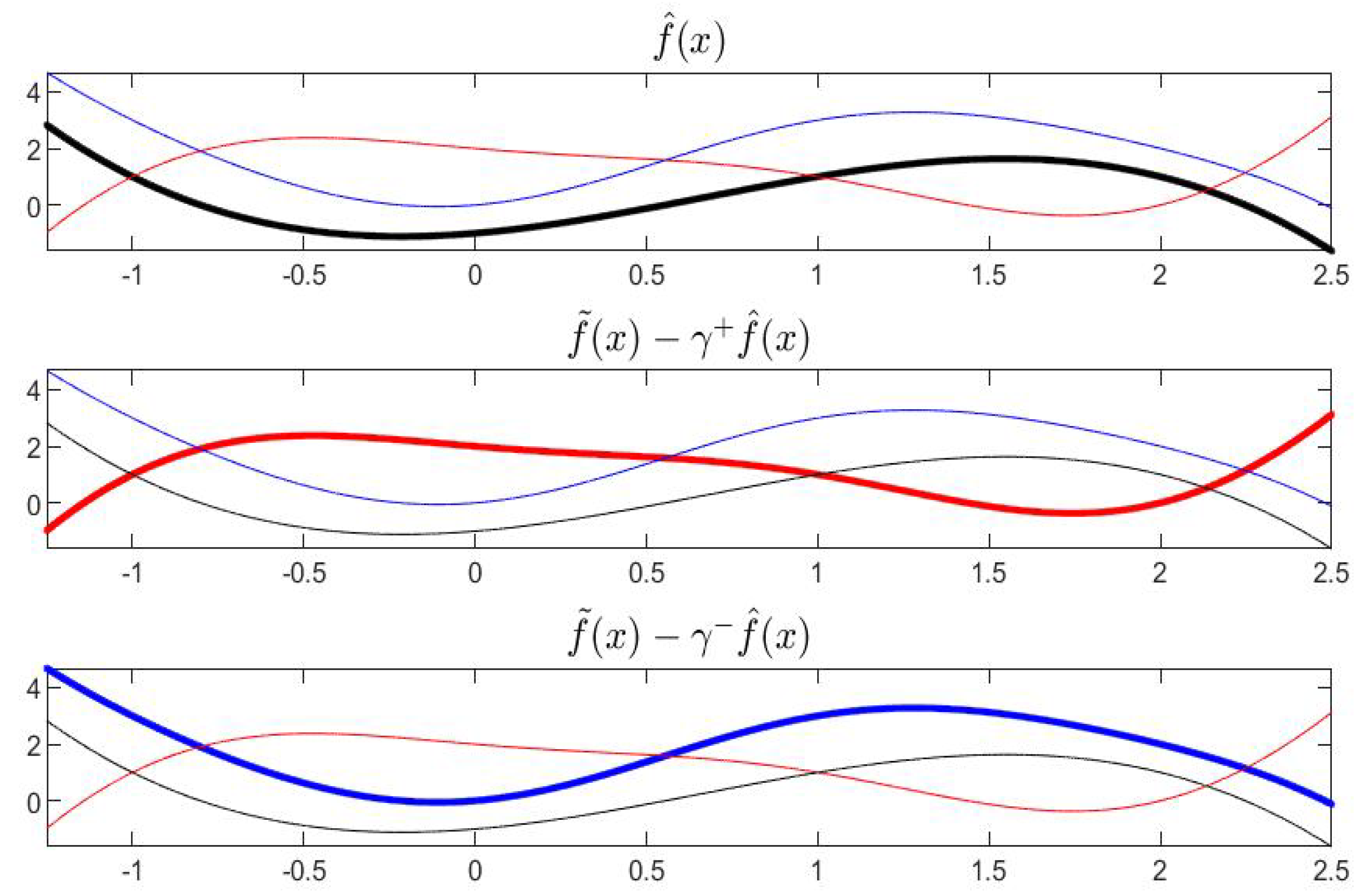
With reference to Example 1, the functions $\widehat{f}(x)$, $\tilde{f}(x)-{\gamma }^{+}\widehat{f}(x)$ and $\tilde{f}(x)-{\gamma }^{-}\widehat{f}(x)$ are pictured in Figure 13 and their derivatives are in Figure 14; the partial order is fixed with ${\gamma }^{-}=-1$ and ${\gamma }^{+}=1$, i.e., ${⪷}_{LU}$.

Now, but only for the case of a partial order ${⪷}_{{\gamma }^{-},{\gamma }^{+}}$ with the condition that ${\gamma }^{-}+{\gamma }^{+}=0$, i.e., ${\gamma }^{+}=-{\gamma }^{-}=\gamma >0$, we can establish a strong connection between the monotonicity of F and the sign of its gH-derivative $F_{gH}^{\prime }(x)$. Denote the corresponding partial order ${⪷}_{-\gamma ,\gamma }$ simply by ${⪷}_{\gamma }$.

Proposition 15.

Let $F:]a,b[\to {\mathcal{K}}_C$ be given, $F(x)=\left(\widehat{f}(x);\tilde{f}(x)\right)$ and assume F has gH-derivative $F_{gH}^{\prime }(x)$ at the internal points $x\in ]a,b[$. Let $\gamma >0$ be fixed. Then

(1) 

If F is $({⪷}_{\gamma })$-nondecreasing on $]a,b[$, then for all x, $F_{gH}^{\prime }(x){⪸}_{\gamma }0$;

(2) 

If F is $({⪷}_{\gamma })$-nonincreasing on $]a,b[$, then for all x, $F_{gH}^{\prime }(x){⪷}_{\gamma }0$.

Proof. 

We prove only (i). By definition, $F_{gH}^{\prime }(x)=\underset{h\to 0}{lim}\frac{1}{h}[F(x+h){\ominus }_{gH}F(x)]$ and F is continuous. If F is nondecreasing, then, for sufficiently small $h>0$ we have $F(x){⪷}_{\gamma }F(x+h)$ and so $0{⪷}_{\gamma }F(x+h){\ominus }_{gH}F(x)$ which gives$0{⪷}_{\gamma }\frac{F(x+h){\ominus }_{gH}F(x)}{h}$; by taking the limit for $h\searrow 0$, $0{⪷}_{\gamma }{F}_{gH}^{\prime }(x)$. On the other hand, for $h<0$, we have $F(x+h){⪷}_{\gamma }F(x)$, i.e., $F(x+h){\ominus }_{gH}F(x){⪷}_{\gamma }0$ which gives$\frac{F(x+h){\ominus }_{gH}F(x)}{-h}{⪷}_{\gamma }0$; by taking the limit for $h\nearrow 0$ we get $(-F_{gH}^{\prime }(x)){⪷}_{\gamma }0$ and, changing sign on both sides, it is $F_{gH}^{\prime }(x){⪸}_{\gamma }0$. The proof of (ii) is similar. □

An analogous result is also immediate, relating strong (local) monotonicity of F to the “sign” of its left and right derivatives $F_{(l)gH}^{\prime }(x)=\left({\widehat{f}}_l^{\prime }(x);\left|{\tilde{f}}_l^{\prime }(x)\right|\right)$ and $F_{(r)gH}^{\prime }(x)=\left({\widehat{f}}_r^{\prime }(x);\left|{\tilde{f}}_r^{\prime }(x)\right|\right)$; at the extreme points of $[a,b]$, we consider only right (at a) or left (at b) monotonicity and right or left derivatives. Again we assume the condition ${\gamma }^{+}=-{\gamma }^{-}=\gamma >0$.

Proposition 16.

Let $F:[a,b]\to {\mathcal{K}}_C$ be given, $F(x)=\left(\widehat{f}(x);\tilde{f}(x)\right)$ with left and/or right gH-derivatives at a point $x_0\in [a,b]$. Then

(i.a) if $0{\prec }_{\gamma }{F}_{(l)gH}^{\prime }(x_0)$, then F is strongly $({\prec }_{\gamma })$-increasing on $[x_0-\delta ,x_0]$ for some $\delta >0$ (here $x_0>a$);

(i.b) if $0{\prec }_{\gamma }{F}_{(r)gH}^{\prime }(x_0)$, then F is strongly $({\prec }_{\gamma })$-increasing on $[x_0,x_0+\delta ]$ for some $\delta >0$ (here $x_0<b$);

(ii.a) if $0{\succ }_{\gamma }{F}_{(l)gH}^{\prime }(x_0)$, then F is strongly $({\prec }_{\gamma })$-decreasing on $[x_0-\delta ,x_0]$ for some $\delta >0$ (here $x_0>a$);

(ii.b) if $0{\succ }_{\gamma }{F}_{(r)gH}^{\prime }(x_0)$, then F is strongly $({\prec }_{\gamma })$-decreasing on $[x_0,x_0+\delta ]$ for some $\delta >0$ (here $x_0<b$).

Proof. 

We prove only (i.a). From $\left({\widehat{f}}_l^{\prime }(x);\left|{\tilde{f}}_l^{\prime }(x)\right|\right){\succ }_{\gamma }0$ we have ${\widehat{f}}_l^{\prime }(x_0)>0$ and $\left|{\tilde{f}}_l^{\prime }(x_0)\right|<\gamma {\widehat{f}}_l^{\prime }(x_0)$, i.e., $-\gamma {\widehat{f}}_l^{\prime }(x_0)<{\tilde{f}}_l^{\prime }(x_0)<\gamma {\widehat{f}}_l^{\prime }(x_0)$; then $0<{\tilde{f}}_l^{\prime }(x_0)+\gamma {\widehat{f}}_l^{\prime }(x_0)$, ${\tilde{f}}_l^{\prime }(x_0)-\gamma {\widehat{f}}_l^{\prime }(x_0)<0$ and the conclusion follows from conditions (38). □

We conclude this section with the following

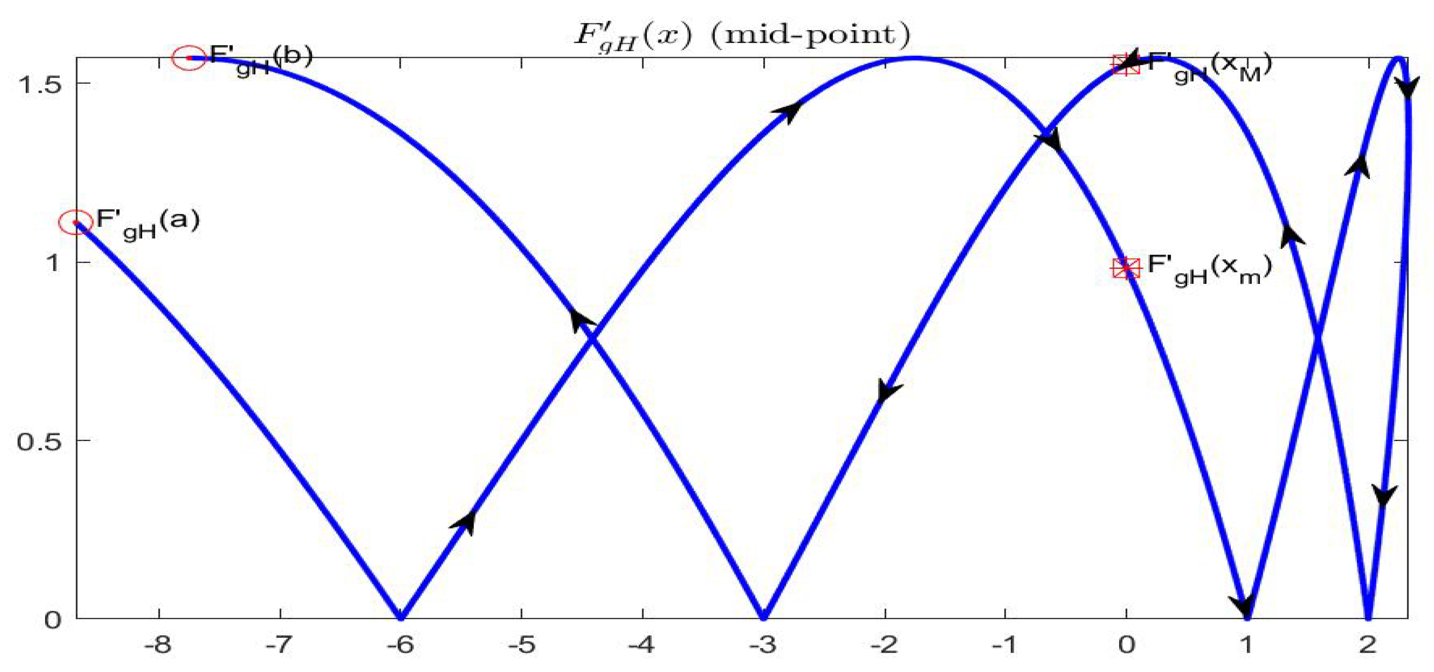
Example 2.

Function $F:[a,b]\to {\mathcal{K}}_C$, $F(x)=\left(\widehat{f}(x);\tilde{f}(x)\right)$, for $x\in [a,b]=[-2,4]$, is defined by $\widehat{f}(x)=-x^3+4x^2+3x-1$ and $\tilde{f}(x)=\left|x^2-x-2\right|$ (Figure 15).

Remark that function $\widehat{f}(x)$ is differentiable on $]a,b[$ with ${\widehat{f}}^{\prime }(x)=-3x^2+8x+3$ and $\tilde{f}(x)$ is differentiable with $\tilde{f}{(x)}^{\prime }=(2x-1)sign(x^2-x-2)$ for $x\ne -1$ and $x\ne 2$; at these two points the left and right derivatives exist: ${\tilde{f}}_l^{\prime }(-1)=-3$, ${\tilde{f}}_r^{\prime }(-1)=3$, ${\tilde{f}}_l^{\prime }(2)=-3$, ${\tilde{f}}_r^{\prime }(2)=3$.

Function $F(x)$ is gH-differentiable on $]a,b[$ (including the points $x=-1$ and $x=2$) and $F_{gH}^{\prime }(x)=\left(-3x^2+8x+3;\left|2x-1\right|\right)$ (Figure 16). Also right and left gH-derivatives exist at $a=-2$ and $b=4$, respectively. Considering the points $a_1=-0.527525$, $a_2=-0.189255$, $a_3=2.527525$ and $a_4=3.522588$, the corresponding gH-derivatives are (approximately) $F_{gH}^{\prime }(a_1)=[-4.11,0]$, $F_{gH}^{\prime }(a_2)=[0,2.757]$, $F_{gH}^{\prime }(a_3)=[0,8.11]$, $F_{gH}^{\prime }(a_1)=[-12.09,0]$.

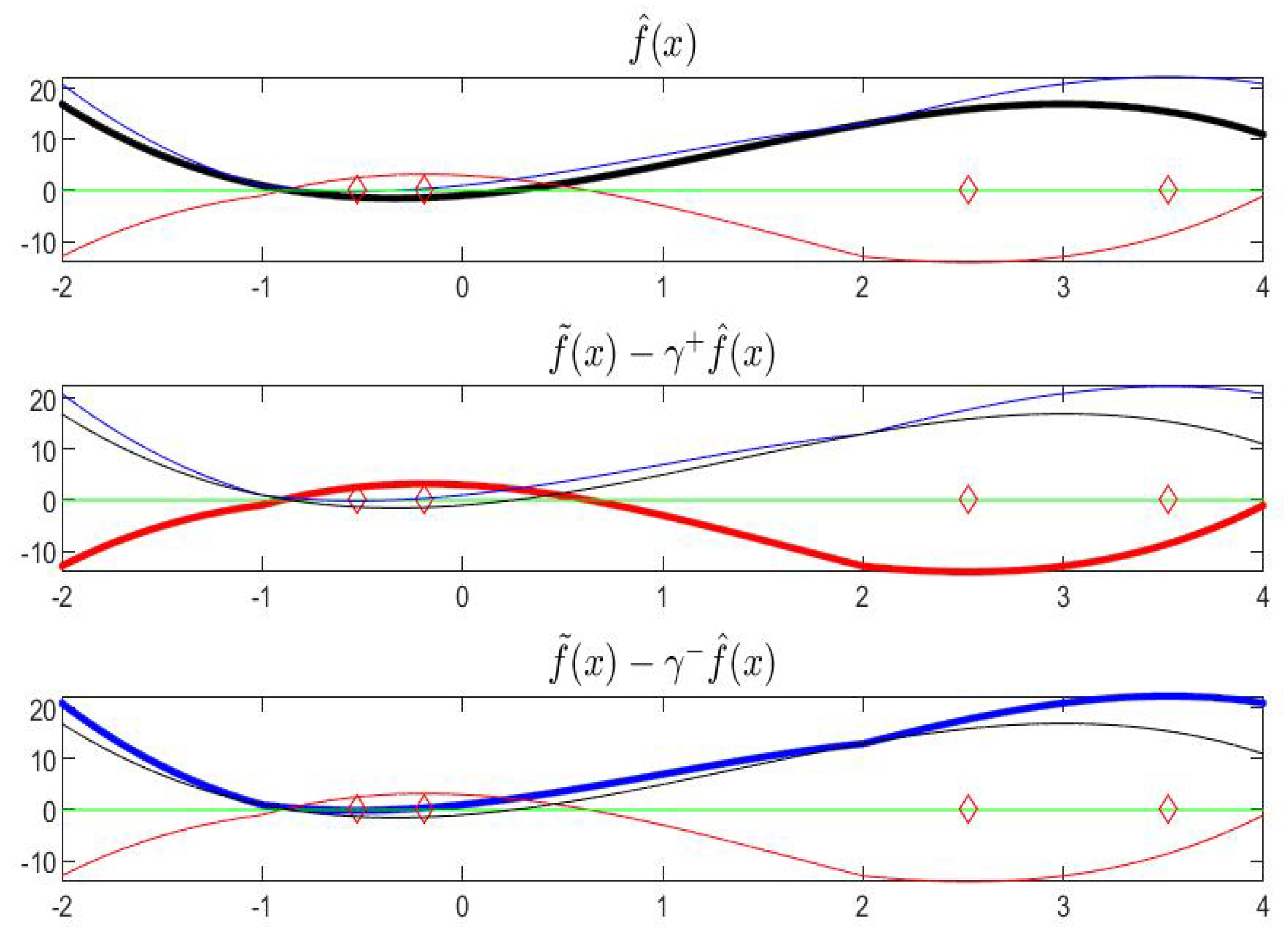
With ${\gamma }^{+}=-{\gamma }^{-}=1$, i.e., with (${⪷}_{LU}$)-order, the functions $\widehat{f}(x)$, $\tilde{f}(x)-{\gamma }^{+}\widehat{f}(x)$ and $\tilde{f}(x)-{\gamma }^{-}\widehat{f}(x)$ are pictured in Figure 17.

According to Proposition 13, necessary conditions for decreasing $F(x)$ are satisfied on $[a,a_1]$ and $[a_4,b]$ and for increasing $F(x)$ are satisfied on $[a_2,a_3]$. Corresponding necessary conditions using the sign of the derivatives of functions $\widehat{f}(x)$, $\tilde{f}(x)-{\gamma }^{+}\widehat{f}(x)$ and $\tilde{f}(x)-{\gamma }^{-}\widehat{f}(x)$ can be checked in Figure 18; at the points $x=-1$ and $x=2$ we can apply the conditions involving left and right derivatives of $\tilde{f}(x)$.

Finally, according to Proposition 16, it is easy to check that the sufficient conditions for strong ${\prec }_{LU}$ monotonicity are satisfied: decreasing on $[-2,a_1]$ and $[a_4,4]$, increasing on $[a_2,a_3]$. In the remaining points $x\in ]a_1,a_2[$ and $x\in ]a_3,a_4[$ the sufficient conditions for strong ${\prec }_{\gamma }$ monotonicity are not satisfied (the interval-valued gH-derivatives of $F(x)$ contain zero as an interior value).

7. Conclusions and Further Work

In the first part of this work we have introduced a general framework for ordering intervals, using a comparison index based on gH-difference; the suggested approach includes most of the partial orders proposed in the literature and preserves important desired properties, including that the space of real intervals is a lattice with the bounded property (all bounded sets of intervals have a supremum and an infimum interval).

The monotonicity properties are defined and analyzed in terms of the suggested partial orders and the relevant connections with gH-derivative are established.

In Part II of the paper, we will further develop new results to define extremal points (local or global minimum or maximum) in terms of the same general partial orders developed in this part and we will analyze the important concepts of concavity and convexity by the use of first-order and second-order gH-derivatives.

Interesting connections with differential geometry and with periodic curves (as in [64,65,66]) will be analyzed.