Gabor Frames and Deep Scattering Networks in Audio Processing


Abstract
1. Introduction
1.1. Convolutional Neural Networks (CNNs) and Invariance
1.2. Invarince Induced by Gabor Scattering
2. Materials and Methods
2.1. Gabor Scattering
- The translation (time shift) operator:
- -
- for a function and is defined as for all
- -
- for a function and is defined as
- The modulation (frequency shift) operator:
- -
- for a function and is defined as for all
- -
- for a function and is defined as
- with is a Gabor frame indexed by a lattice
- A nonlinearity function (e.g., rectified linear units, modulus function, see [4]) is applied pointwise and is chosen to be Lipschitz-continuous, i.e., for all In this paper we only use the modulus function with Lipschitz constant for all
- Pooling depends on a pooling factor which leads to dimensionality reduction. Mostly used are max- or average-pooling, some more examples can be found in [4]. In our context, pooling is covered by choosing specific lattices in each layer.
2.2. Musical Signal Model
3. Theoretical Results
3.1. Gabor Scattering of Music Signals
3.1.1. Invariance
3.1.2. Deformation Stability
- envelope changesfor depending only on
- frequency modulation
3.2. Visualization Example
3.2.1. Visualization of Different Frequency Channels within the GS Implementation
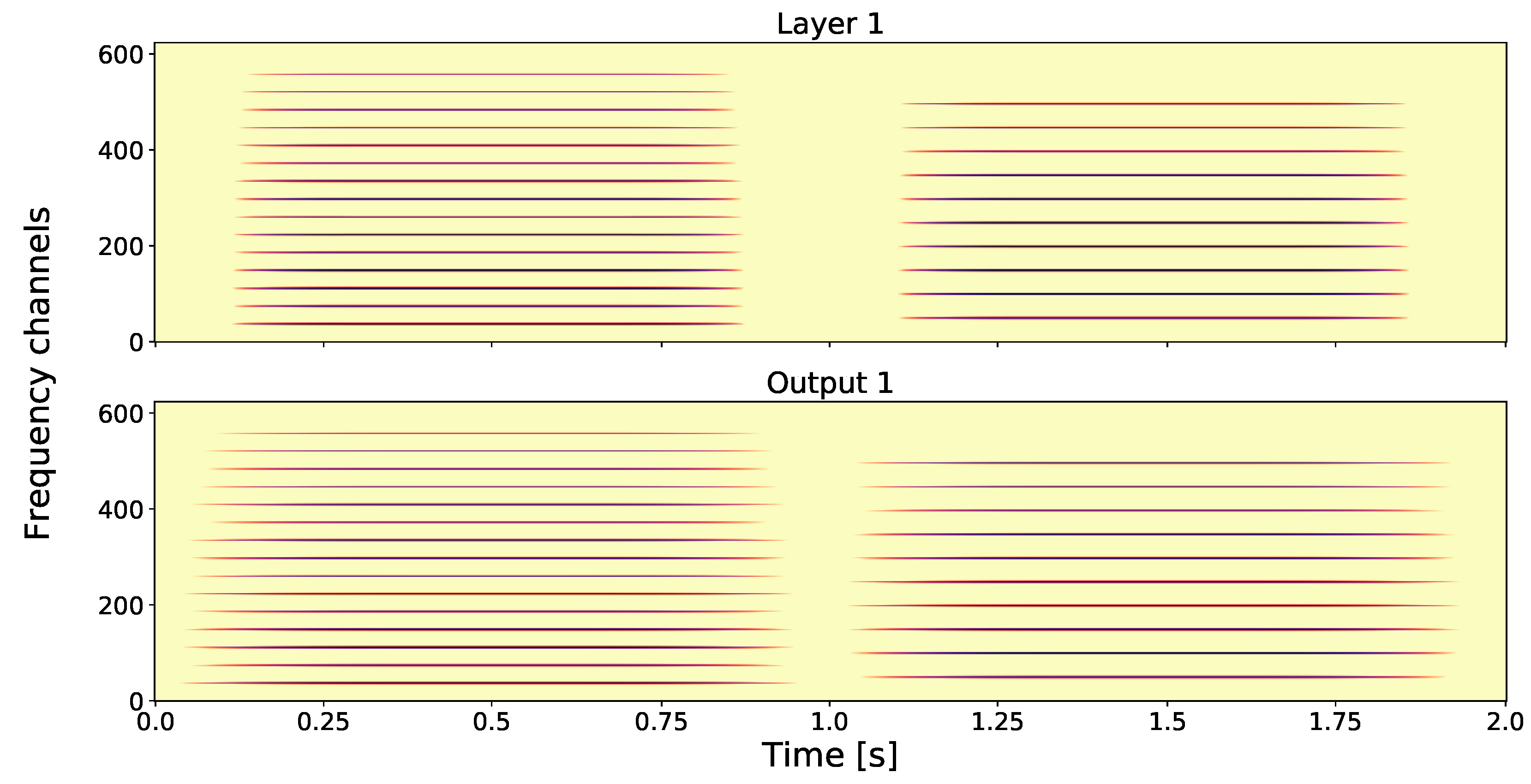
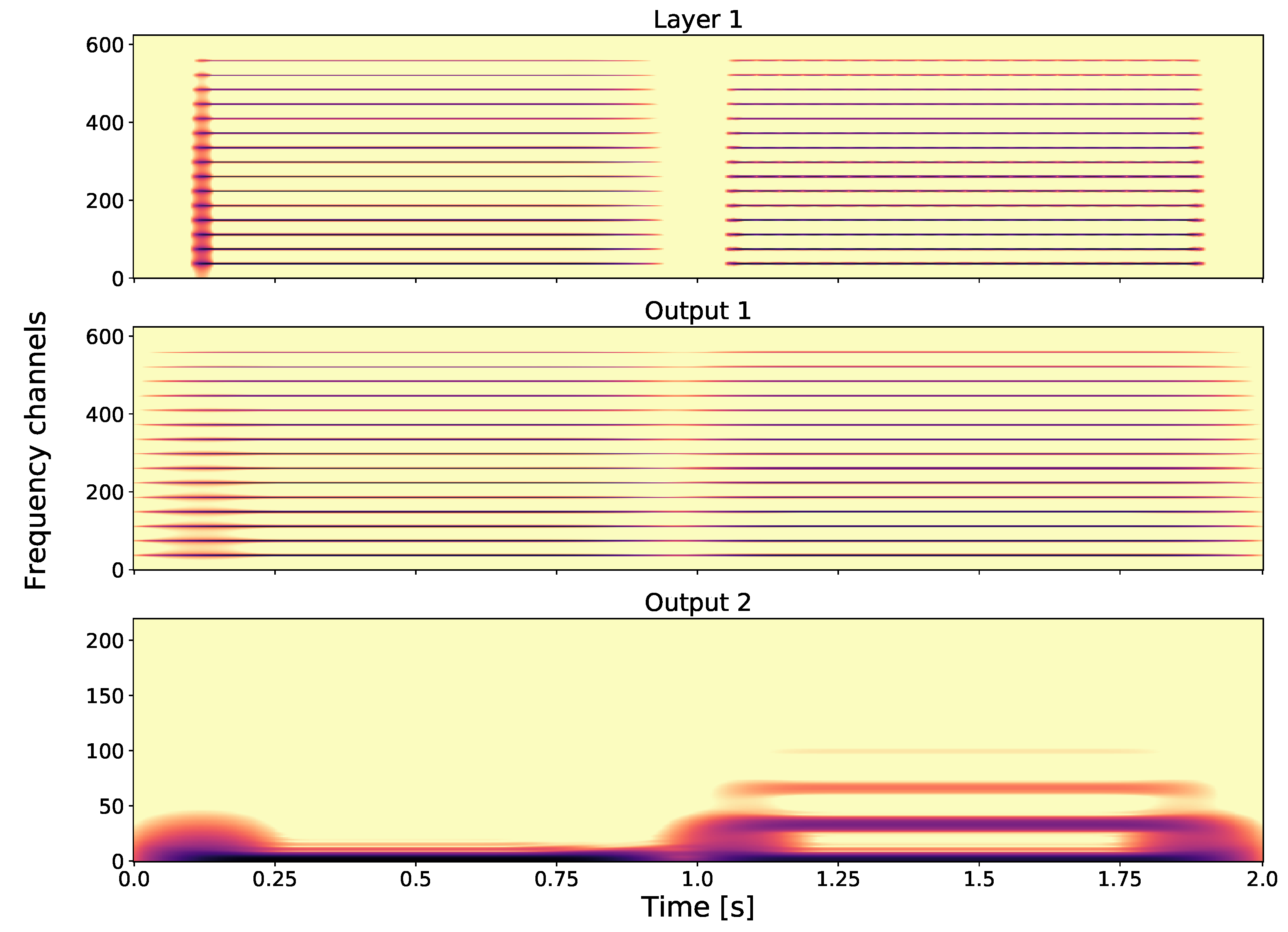
- Layer 1: The first spectrogram of Figure 3 shows the GT. Observe the difference in the fundamental frequencies and that these two tones have a different number of harmonics, i.e., tone one has more than tone two.
- Output 1: The second spectrogram of Figure 3 shows Output 1, which is is time averaged version of Layer 1.
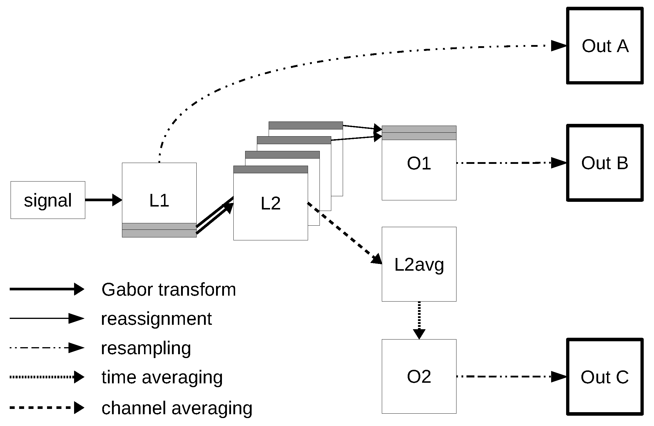
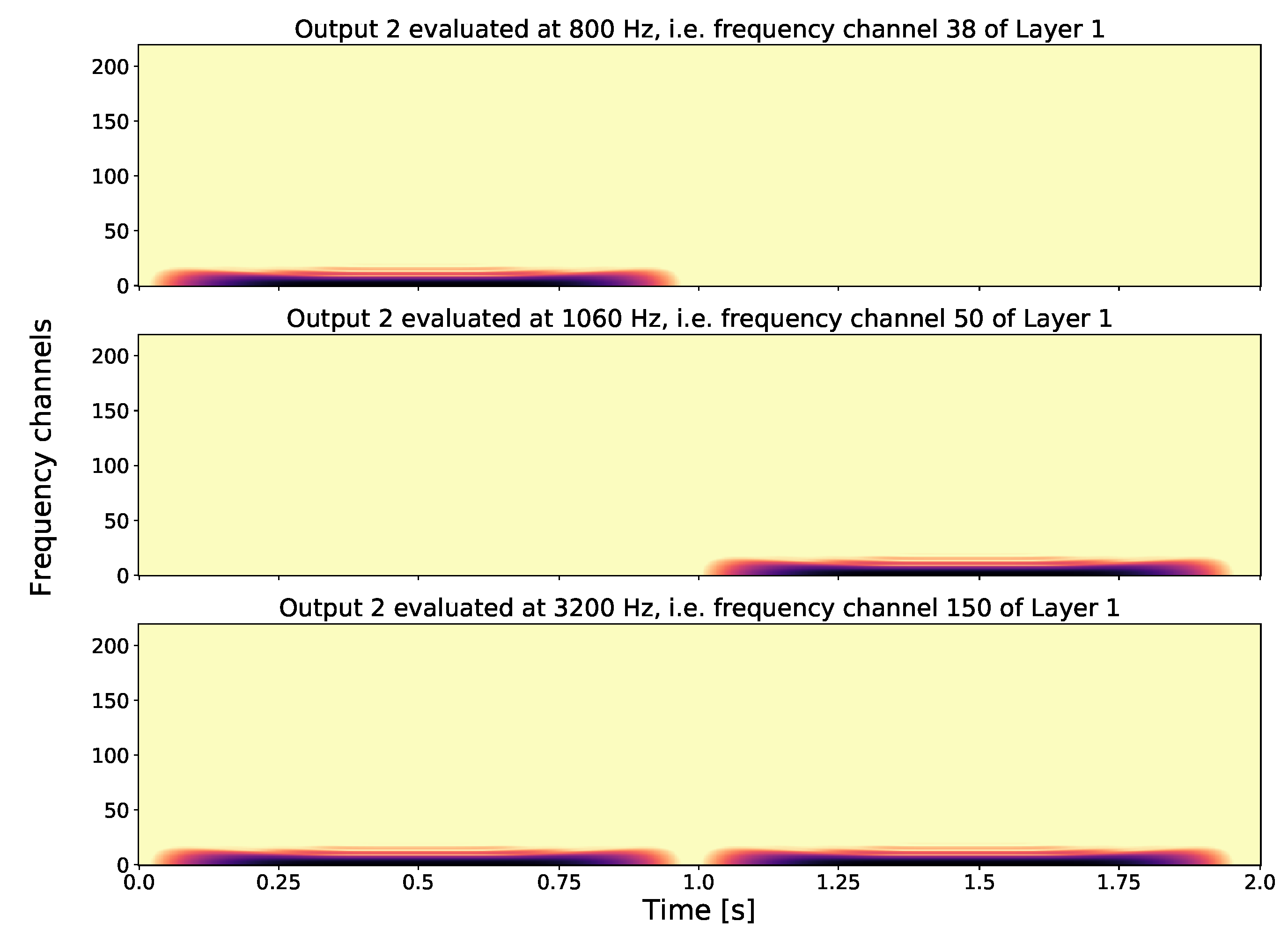
- Output 2: For the second layer output (see Figure 4), we take a fixed frequency channel from Layer 1 and compute another GT to obtain a Layer 2 element. By applying an output-generating atom, i.e., a low-pass filter, we obtain Output 2. Here, we show how different frequency channels of Layer 1 can affect Output 2. The first spectrogram shows Output 2 with respect to, the fundamental frequency of tone one, i.e., Therefore no second tone is visible in this output. On the other hand, in the second spectrogram, if we take as fixed frequency channel in Layer 1 the fundamental frequency of the second tone, i.e., in Output 2, the first tone is not visible. If we consider a frequency that both share, i.e., , we see that for Output 2 in the third spectrogram both tones are present. As GS focuses on one frequency channel in each layer element, the frequency information in this layer is lost; in other words, Layer 2 is invariant with respect to frequency.
3.2.2. Visualization of Different Envelopes within the GS Implementation
- Layer 1: In the spectrogram showing the GT, we see the difference between the envelopes and we see that the signals have the same pitch and the same harmonics.
- Output 1: The output of the first layer is invariant with respect to the envelope of the signals. This is due to the output-generating atom and the subsampling, which removes temporal information of the envelope. In this output, no information about the envelope (neither the sharp attack nor the amplitude modulation) is visible, therefore the spectrogram of the different signals look almost the same.
- Output 2: For the second layer output we took as input a time vector at fixed frequency of 800 Hz (i.e., frequency channel 38) of the first layer. Output 2 is invariant with respect to the pitch, but differences on larger scales are captured. Within this layer we are able to distinguish the different envelopes of the signals. We first see the sharp attack of the first tone and then the modulation with a second frequency is visible.
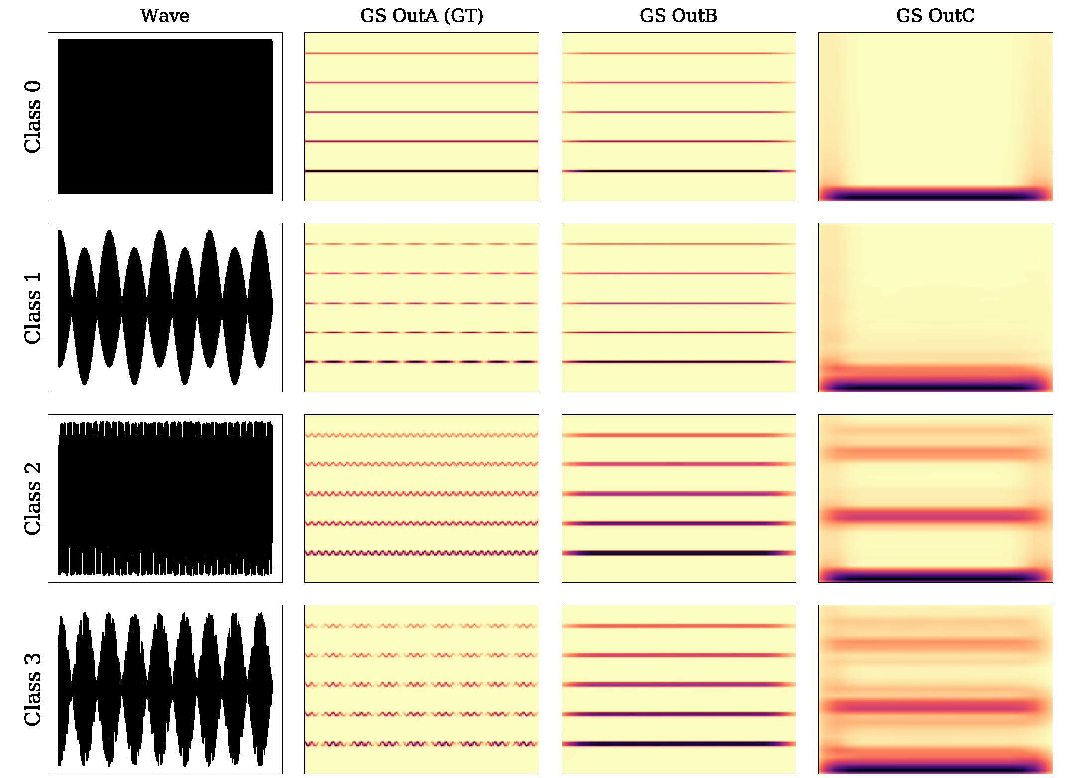
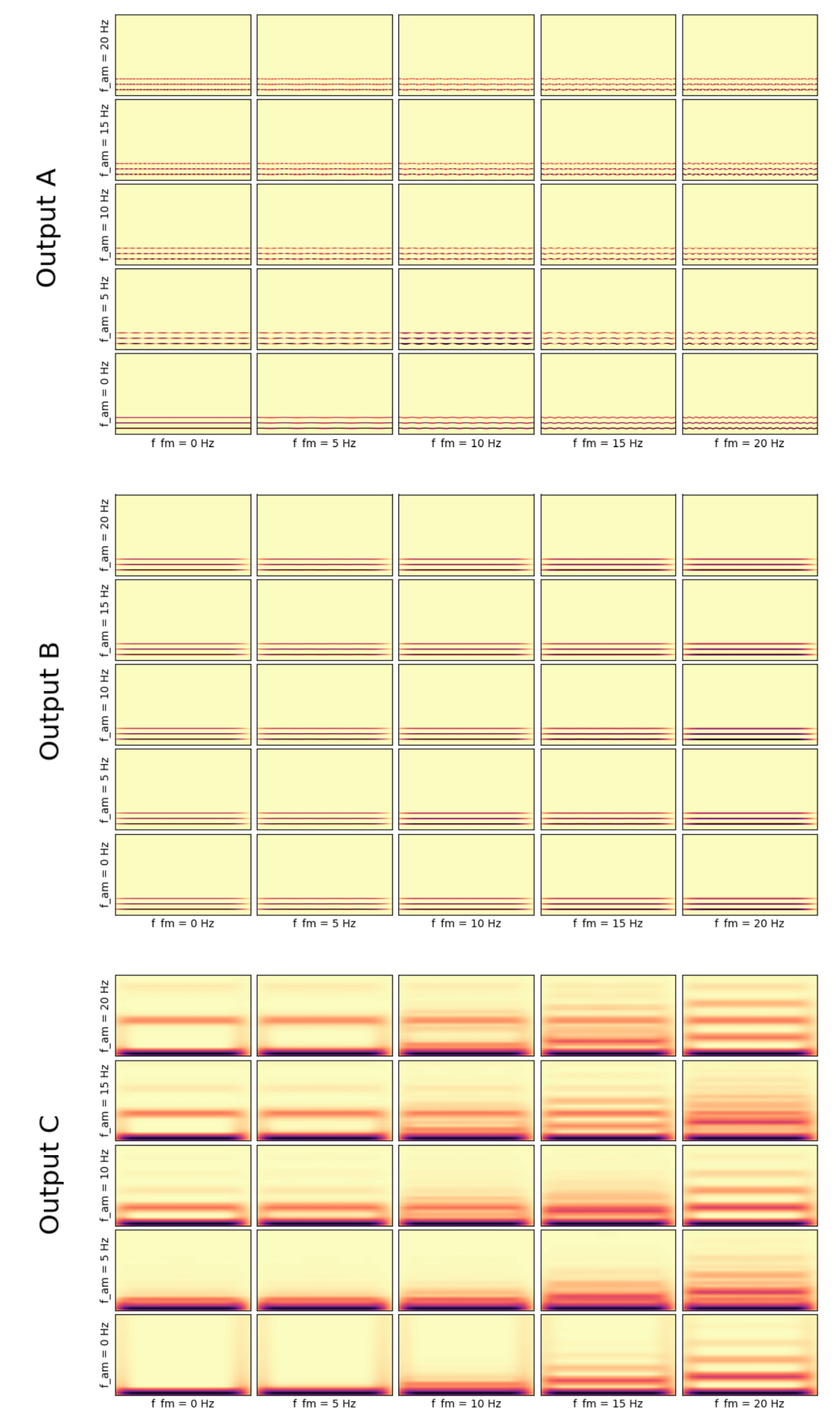
3.2.3. Visualization of How Frequency and Amplitude Modulations Influence the Outputs Using the Channel Averaged Implementation
4. Experimental Results
4.1. Experiments with Synthetic Data
4.1.1. Data
4.1.2. Training
4.1.3. Results
4.2. Experiments with GoodSounds Data
4.2.1. Data
4.2.2. Training
4.2.3. Results
5. Discussion and Future Work
Author Contributions
Funding
Conflicts of Interest
References
- Krizhevsky, A.; Sutskever, I.; Hinton, G.E. ImageNet Classification with Deep Convolutional Neural Networks. In Advances in Neural Information Processing Systems 25; Pereira, F., Burges, C.J.C., Bottou, L., Weinberger, K.Q., Eds.; Curran Associates, Inc.: Red Hook, NY, USA, 2012; pp. 1097–1105. [Google Scholar]
- Grill, T.; Schlüter, J. Music Boundary Detection Using Neural Networks on Combined Features and Two-Level Annotations. In Proceedings of the 16th International Society for Music Information Retrieval Conference (ISMIR 2015), Malaga, Spain, 26–30 October 2015. [Google Scholar]
- Mallat, S. Group Invariant Scattering. Comm. Pure Appl. Math. 2012, 65, 1331–1398. [Google Scholar] [CrossRef]
- Wiatowski, T.; Bölcskei, H. A Mathematical Theory of Deep Convolutional Neural Networks for Feature Extraction. IEEE Trans. Inf. Theory 2017, 64, 1845–1866. [Google Scholar] [CrossRef]
- Wiatowski, T.; Bölcskei, H. Deep Convolutional Neural Networks Based on Semi-Discrete Frames. In Proceedings of the IEEE International Symposium on Information Theory (ISIT), Hong Kong, China, 14–19 June 2015; pp. 1212–1216. [Google Scholar]
- Andén, J.; Mallat, S. Deep Scattering Spectrum. IEEE Trans. Signal Process. 2014, 62, 4114–4128. [Google Scholar] [CrossRef]
- Andén, J.; Lostanlen, V.; Mallat, S. Joint time-frequency scattering for audio classification. In Proceedings of the 2015 IEEE 25th International Workshop on Machine Learning for Signal Processing (MLSP), Boston, MA, USA, 17–20 September 2015; pp. 1–6. [Google Scholar]
- Grohs, P.; Wiatowski, T.; Bölcskei, H. Deep convolutional neural networks on cartoon functions. In Proceedings of the 2016 IEEE International Symposium on Information Theory (ISIT), Barcelona, Spain, 10–15 July 2016; pp. 1163–1167. [Google Scholar]
- Romani Picas, O.; Parra Rodriguez, H.; Dabiri, D.; Tokuda, H.; Hariya, W.; Oishi, K.; Serra, X. A real-time system for measuring sound goodness in instrumental sounds. In Audio Engineering Society Convention 138; Audio Engineering Society: New York, NY, USA, 2015. [Google Scholar]
- Zhang, C.; Bengio, S.; Hardt, M.; Recht, B.; Vinyals, O. Understanding deep learning requires rethinking generalization. arXiv 2016, arXiv:1611.03530. [Google Scholar]
- Kawaguchi, K.; Kaelbling, L.P.; Bengio, Y. Generalization in Deep Learning. arXiv 2017, arXiv:1710.05468. [Google Scholar]
- Hofmann, T.; Schölkopf, B.; Smola, A. Kernel Methods in Machine Learning. Ann. Stat. 2008, 36, 1171–1220. [Google Scholar] [CrossRef]
- Mallat, S. Understanding deep convolutional networks. Philos. Trans. R. Soc. Lond. A Math. Phys. Eng. Sci. 2016, 374. [Google Scholar] [CrossRef] [PubMed]
- Wiatowski, T.; Tschannen, M.; Stanic, A.; Grohs, P.; Bölcskei, H. Discrete deep feature extraction: A theory and new architectures. In Proceedings of the International Conference on Machine Learning (ICML), New York, NY, USA, 19–24 June 2016. [Google Scholar]
- Gröchenig, K. Foundations of Time-Frequency Analysis; Applied and Numerical Harmonic Analysis; Birkhäuser: Boston, MA, USA; Basel, Switzerland; Berlin, Germany, 2001. [Google Scholar]
- Harar, P.; Bammer, R. gs-gt. Available online: https://gitlab.com/hararticles/gs-gt (accessed on 20 June 2019).
- Harar, P. Gabor Scattering v0.0.4. Available online: https://gitlab.com/paloha/gabor-scattering (accessed on 20 June 2019).
- Jones, E.; Oliphant, T.; Peterson, P. SciPy: Open Source Scientific Tools for Python. 2001. Available online: http://www.scipy.org/ (accessed on 1 February 2019).
- Oppenheim, A.V. Discrete-Time Signal Processing; Pearson Education India: Uttar Pradesh, India, 1999. [Google Scholar]
- Griffin, D.; Lim, J. Signal estimation from modified short-time Fourier transform. IEEE Trans. Acoust. Speech Signal Process. 1984, 32, 236–243. [Google Scholar] [CrossRef]
- Kirkland, E.J. Bilinear interpolation. In Advanced Computing in Electron Microscopy; Springer: Berlin/Heidelberg, Germany, 2010; pp. 261–263. [Google Scholar]
- Glorot, X.; Bengio, Y. Understanding the difficulty of training deep feedforward neural networks. Aistats 2010, 9, 249–256. [Google Scholar]
- He, K.; Zhang, X.; Ren, S.; Sun, J. Delving Deep into Rectifiers: Surpassing Human-Level Performance on ImageNet Classification. In Proceedings of the IEEE International Conference on Computer Vision (ICCV), Santiago, Chile, 7–13 December 2015. [Google Scholar]
- Goodfellow, I.; Bengio, Y.; Courville, A. Deep Learning; MIT Press: Cambridge, MA, USA, 2016. [Google Scholar]
- Kingma, D.; Ba, J. Adam: A method for stochastic optimization. arXiv 2014, arXiv:1412.6980. [Google Scholar]
- Chollet, F. Keras. Available online: https://keras.io (accessed on 19 August 2019).
- Abadi, M.; Agarwal, A.; Barham, P.; Brevdo, E.; Chen, Z.; Citro, C.; Corrado, C.; Davis, A.; Dean, J.; Devin, M.; et al. TensorFlow: Large-Scale Machine Learning on Heterogeneous Systems. 2015. Available online: https://www.tensorflow.org (accessed on 1 February 2019 ).
- Bagwell, C. SoX—Sound Exchange the Swiss Army Knife of Sound Processing. Available online: https://launchpad.net/ubuntu/+source/sox/14.4.1-5 (accessed on 31 October 2018).
- Navarrete, J. The SoX of Silence Tutorial. Available online: https://digitalcardboard.com/blog/2009/08/25/the-sox-of-silence (accessed on 31 October 2018).
- Bammer, R.; Breger, A.; Dörfler, M.; Harar, P.; Smékal, Z. Machines listening to music: The role of signal representations in learning from music. arXiv 2019, arXiv:1903.08950. [Google Scholar]
| 1. | We point out that the term kernel as used in this work always means convolutional kernels in the sense of filterbanks. Both the fixed kernels used in the scattering transform and the kernels used in the CNNs, whose size is fixed but whose elements are learned, should be interpreted as convolutional kernels in a filterbank. This should not be confused with the kernels used in classical machine learning methods based on reproducing kernel Hilbert spaces, e.g., the famous support vector machine, c.f. [12] |
| 2. | In general, one could take As this element is the ℓ-th convolution, it is an element of the ℓ-th frame, but because it belongs to the -th layer, its index is . |


| = 0 | = 1 | |
| class 0 | class 1 | |
| = 1 | class 2 | class 3 |
| TF | N Train | N Valid | BWU | Train | Valid |
|---|---|---|---|---|---|
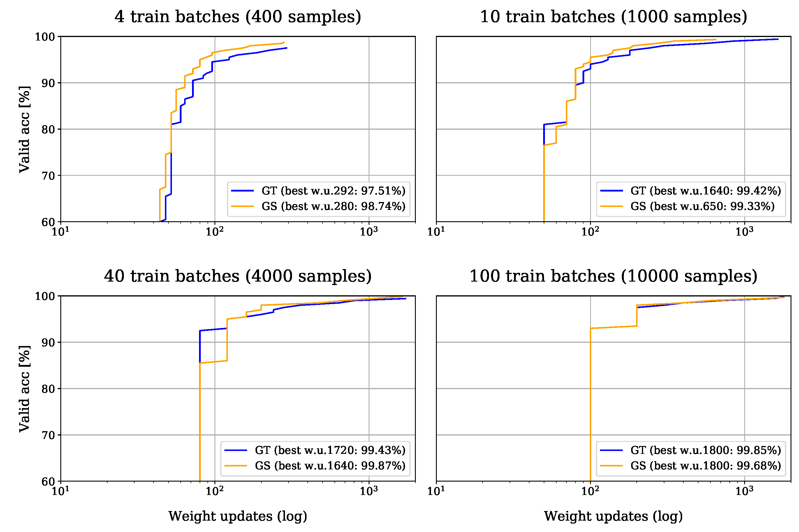
| GS | 400 | 20,000 | 280 | 1.0000 | 0.9874 |
| GT | 400 | 20,000 | 292 | 1.0000 | 0.9751 |
| GS | 1000 | 20,000 | 650 | 0.9990 | 0.9933 |
| GT | 1000 | 20,000 | 1640 | 1.0000 | 0.9942 |
| GS | 4000 | 20,000 | 1640 | 0.9995 | 0.9987 |
| GT | 4000 | 20,000 | 1720 | 0.9980 | 0.9943 |
| GS | 10,000 | 20,000 | 1800 | 0.9981 | 0.9968 |
| GT | 10,000 | 20,000 | 1800 | 0.9994 | 0.9985 |
| All Available Data | Obtained Segments | |||||||
|---|---|---|---|---|---|---|---|---|
| Class | Files | Dur | Ratio | Stride | Train | Valid | Test | |
| Used | Clarinet | 3358 | 369.70 | 21.58% | 37,988 | 12,134 | 4000 | 4000 |
| Flute | 2308 | 299.00 | 17.45% | 27,412 | 11,796 | 4000 | 4000 | |
| Trumpet | 1883 | 228.76 | 13.35% | 22,826 | 11,786 | 4000 | 4000 | |
| Violin | 1852 | 204.34 | 11.93% | 19,836 | 11,707 | 4000 | 4000 | |
| Sax alto | 1436 | 201.20 | 11.74% | 19,464 | 11,689 | 4000 | 4000 | |
| Cello | 2118 | 194.38 | 11.35% | 15,983 | 11,551 | 4000 | 4000 | |
| Not used | Sax tenor | 680 | 63.00 | 3.68% | ||||
| Sax soprano | 668 | 50.56 | 2.95% | |||||
| Sax baritone | 576 | 41.70 | 2.43% | |||||
| Piccolo | 776 | 35.02 | 2.04% | |||||
| Oboe | 494 | 19.06 | 1.11% | |||||
| Bass | 159 | 6.53 | 0.38% | |||||
| Total | 16,308 | 1713.23 | 100.00% | 70,663 | 24,000 | 24,000 | ||
| TF | N Train | N Valid | N Test | BWU | Train | Valid | Test |
|---|---|---|---|---|---|---|---|
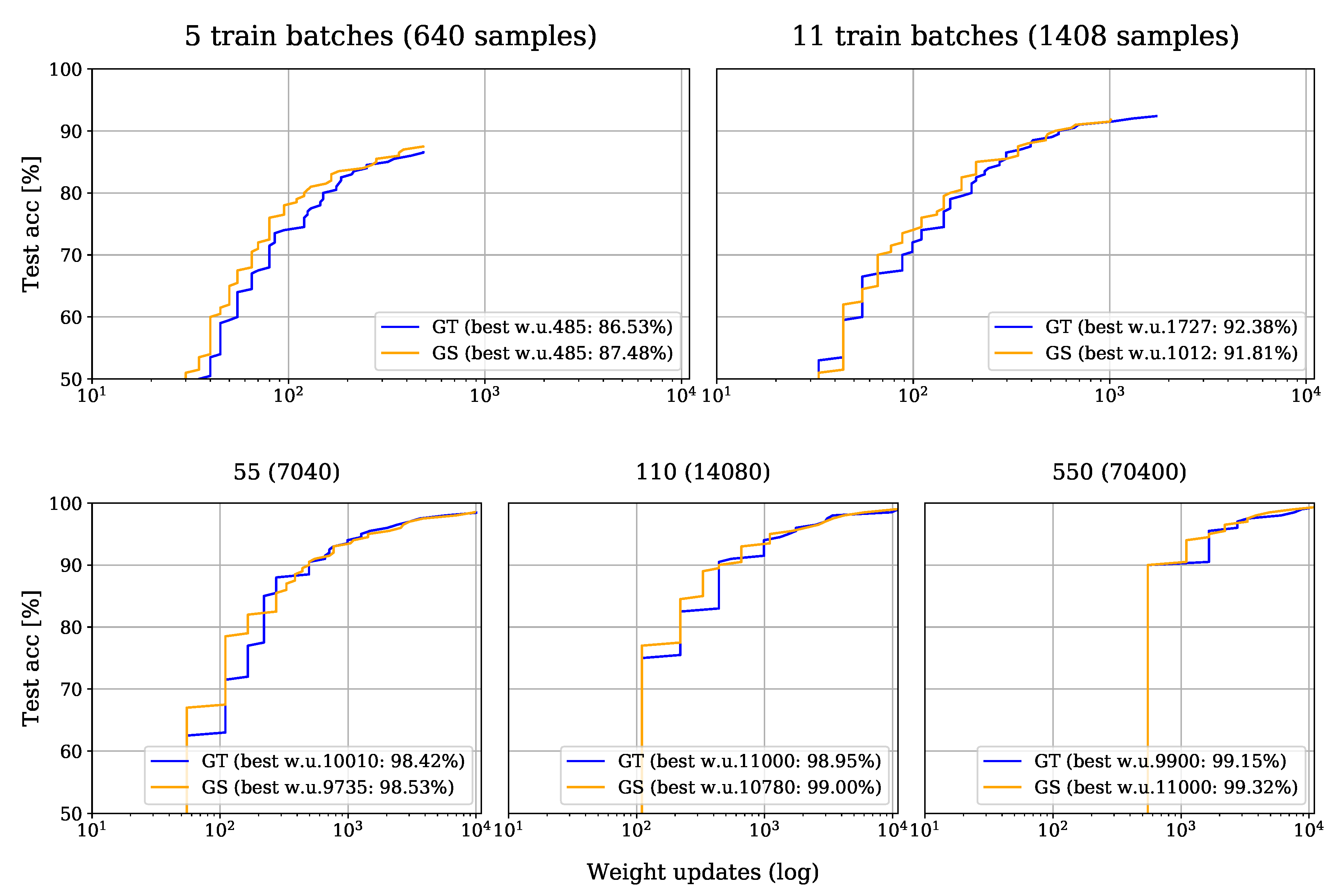
| GS | 640 | 24,000 | 24,000 | 485 | 0.9781 | 0.8685 | 0.8748 |
| GT | 640 | 24,000 | 24,000 | 485 | 0.9766 | 0.8595 | 0.8653 |
| GS | 1408 | 24,000 | 24,000 | 1001 | 0.9773 | 0.9166 | 0.9177 |
| GT | 1408 | 24,000 | 24,000 | 1727 | 0.9943 | 0.9194 | 0.9238 |
| GS | 7040 | 24,000 | 24,000 | 9735 | 0.9996 | 0.9846 | 0.9853 |
| GT | 7040 | 24,000 | 24,000 | 8525 | 0.9999 | 0.9840 | 0.9829 |
| GS | 14,080 | 24,000 | 24,000 | 10,780 | 0.9985 | 0.9900 | 0.9900 |
| GT | 14,080 | 24,000 | 24,000 | 9790 | 0.9981 | 0.9881 | 0.9883 |
| GS | 70,400 | 24,000 | 24,000 | 11,000 | 0.9963 | 0.9912 | 0.9932 |
| GT | 70,400 | 24,000 | 24,000 | 8800 | 0.9934 | 0.9895 | 0.9908 |
© 2019 by the authors. Licensee MDPI, Basel, Switzerland. This article is an open access article distributed under the terms and conditions of the Creative Commons Attribution (CC BY) license (http://creativecommons.org/licenses/by/4.0/).
Share and Cite
Bammer, R.; Dörfler, M.; Harar, P. Gabor Frames and Deep Scattering Networks in Audio Processing. Axioms 2019, 8, 106. https://doi.org/10.3390/axioms8040106
Bammer R, Dörfler M, Harar P. Gabor Frames and Deep Scattering Networks in Audio Processing. Axioms. 2019; 8(4):106. https://doi.org/10.3390/axioms8040106
Chicago/Turabian StyleBammer, Roswitha, Monika Dörfler, and Pavol Harar. 2019. "Gabor Frames and Deep Scattering Networks in Audio Processing" Axioms 8, no. 4: 106. https://doi.org/10.3390/axioms8040106
APA StyleBammer, R., Dörfler, M., & Harar, P. (2019). Gabor Frames and Deep Scattering Networks in Audio Processing. Axioms, 8(4), 106. https://doi.org/10.3390/axioms8040106