Sumudu Decomposition Method for Solving Fuzzy Integro-Differential Equations

Abstract

Different results regarding different integro-differentials are usually not properly generalized, as they often do not satisfy some of the constraints. The field of fuzzy integro-differentials is very rich these days because of their different applications and functions in different physical phenomena. Solutions of linear fuzzy Volterra integro-differential equations (FVIDEs) are more generalized and have better applications. In this report, the Sumudu decomposition method (SDM) was used to find the solution to some linear and nonlinear fuzzy integro-differential equations (FIDEs). Some examples are given to show the validity of the presented method.

1. Introduction

Linear and nonlinear phenomena are a fundamental part of science and construction. Nonlinear equations are seen in an alternative way when dealing with physical problems such as liquid elements, plasma material science, strong mechanics, quantum field hypotheses, the proliferation of shallow water waves, and numerous other models, all of which are to found within the field of incomplete differential equations. The wide use of these equations is the key to why they have drawn the attention of mathematicians. Regardless of this, they are difficult to solve, either numerically or theoretically. Previously, dynamic examinations were much examined for the potential of finding exact or approximate solutions to these sorts of equations [1,2].

In the recent years, the area of FIDEs has developed a lot and plays a key role in the field of engineering. The elementary impression and arithmetic of fuzzy sets were first introduced by Zadeh. Later, the area of fuzzy derivative and fuzzy integration was studied, and some general results were developed. Fuzzy differential equations (FDEs) and FIDEs are very important in the study of fuzzy theory and have many beneficial consequences related to different problems. Modeling of different physical systems in the differential way gives us different FIDEs [2,3]. Furthermore, FIDEs in a fuzzy setting are a natural way to model the ambiguity of dynamic systems. Consequently, different scientific fields, such as physics, geography, medicine, and biology, pay much importance to the solution of different FIDEs. Solutions to these equations can be utilized in different engineering problems. Seikkala first defined fuzzy derivatives, while the concept of integration of fuzzy functions was first introduced by Dubois and Prade. However, analytic solutions to nonlinear FIDE types are often difficult to find. Therefore, most of the time, an approximate solution is required. There are also useful numerical schemes that can produce a numerical approximation to solutions for some problems [4,5].

The literature on numerical solutions of integro-differential equations (IDEs) is vast. We used the Sumudu decomposition method [6,7,8] to solve linear and nonlinear fuzzy integral equations (FIEs). The method gives more realistic series solutions that converge very rapidly in physical problems. Sumudu transforms are also used for solving IDEs, which can be seen in [4,5]. IDEs are transforms to FIDEs that are more general and give better results. After applying a Sumudu transform, a decomposition method is used for the approximate solution [8,9].

2. Preliminaries

Integral Equation (IE)

The obscure function ${\rm Y}\left(\xi \right)$ that shows up under an integral symbol is known as an integral equation. Usually, we write an integral equation as follow:

$${\rm Y}\left(\xi \right)=f\left(\xi \right)+{\displaystyle \underset{g\left(\xi \right)}{\overset{h\left(\xi \right)}{\int }}}K\left(\xi ,t\right){\rm Y}\left(t\right)dt,$$

(1)

where $k\left(\xi ,t\right)$ and $\lambda$ are the kernel and constant parameter, respectively. The kernel is identified as the function of dual variables $\xi$ and $t$, whereas $g\left(\xi \right)$ and $h\left(\xi \right)$ are recognized as the limitations for integration. The function ${\rm Y}\left(\xi \right)$ to be resolved shows up under the integral symbol; it has the property of appearing in both the outside as well as inside of the integral symbol. The functions that will be specified in progressive are $f\left(\xi \right)$ and $k\left(\xi ,t\right)$. Limitations of integration can adopt both forms, either as the variable, constant, or blended [10].

Types of Integral Equation

IEs show up in numerous forms. Different sorts are generally contingent on the limitations of antiderivatives as well as the kernel of equality. In this content, we focus on the following sorts of IE [11]:

• Fredholm IE;
• Volterra IE;
• Volterra-Fredholm IE;
• Singular.

Volterra Integral Equations (VIEs)

There is a restriction for the VIE, which is that at least one limit should be a variable. Likewise, in FIEs, there are two varieties of VIEs, which are more easily described through the following:

$$f\left(\xi \right)={\displaystyle \underset{0}{\overset{\xi }{\int }}}K\left(\xi ,t\right){\rm Y}\left(t\right)dt.$$

(2)

Equation (2) is a VIE of the first kind.

That is:

$$\xi e^{-\xi }={\displaystyle \underset{0}{\overset{\xi }{\int }}}{e}^{t-\xi }{\rm Y}\left(t\right)dt$$

$${\rm Y}\left(\xi \right)=f\left(\xi \right)+\lambda {\displaystyle \underset{0}{\overset{\xi }{\int }}}K\left(\xi ,t\right){\rm Y}\left(t\right)dt$$

(3)

Equality (3) is a VIE of 2nd type.

For illustration,

$${\rm Y}\left(\xi \right)=1-{\displaystyle \underset{0}{\overset{\xi }{\int }}}{\rm Y}\left(t\right)dt$$

Classification of Integro-Differential Equations

Different types of dynamical physical problems possess integro-differential equations, specifically during the conversion of initial value problems (IVPs) and boundary value problems (BVPs). Differential operators as well as integral operators are involved in an integro-differential equation. There could be any order for the presence of derivatives of the unknown function. In characterizing integro-differential equations, we pursued a similar class as used previously. The following are well-known types of integro-differential equations:

• Fredholm integro-differential equations;
• Volterra integro-differential equations;
• Volterra–Fredholm integro-differential equations.

Volterra Integro-Differential Equation

The Volterra integro-differential equation appears during the conversion of IVPs into the integral equation. In the Volterra integro-differential equation, the unidentified function and its derivatives appear inside as well as outside of the integral operator. For VIE, at least one limit of integration is variable. In order to obtain the exact solution, we need initial conditions in the Volterra integro-differential equation (VIDE). Consider the following VIDE:

$${{\rm Y}}^n\left(\xi \right)=f\left(\xi \right)+\lambda {\displaystyle \underset{0}{\overset{\xi }{\int }}}K\left(\xi ,t\right){\rm Y}\left(t\right)dt$$

(4)

where ${{\rm Y}}^n$ denotes the derivative of order n of ${\rm Y}\left(\xi \right)$. The VIDE given in Equation (4) can be written as:

$${{\rm Y}}^{\prime }\left(\xi \right)=3+\frac{1}{4}{\xi }^2-\xi e^{\xi }-{\displaystyle \underset{0}{\overset{\xi }{\int }}}t{\rm Y}\left(t\right)dt,{\rm Y}\left(0\right)=0,$$

(5)

3. Theorems and Definitions Interrelated to Fuzzy Perceptions

Fuzzy Number

A fuzzy number is a generalization of a regular, real number in the sense that it does not refer to one single value but rather to a connected set of possible values, where each possible value has its own weight between 0 and 1. This weight is called the membership function.

Let E be the set of all fuzzy numbers which upper semicontinuous and compact. The $\alpha$ level set ${\left[{\rm Y}\right]}_{\rho }$ where ${\rm Y}$ is the collection of fuzzy numbers, $0<\rho \le 1$, is defined as:

$${\left[{\rm Y}\right]}_{\rho }=\left\{t\in R,{\rm Y}\left(t\right)\ge \rho \right\}$$

The set E is convex if ${\rm Y}\left(t\right)\ge {\rm Y}\left(s\right)\wedge {\rm Y}\left(r\right)=\min \left({\rm Y}\left(s\right),{\rm Y}\left(r\right)\right),\mathrm{where}s<t<r$.

If $\exists t_o\in R$ such that ${\rm Y}\left(t_o\right)=1,$ then E becomes normal. E is said to be upper semicontinuous if for every $\epsilon >0,suchthat{{\rm Y}}^{-1}\left(\left[0,a+\epsilon \right)\right)$, $\forall a\in \left[0,1\right]$ is open in the typical topology of R [12,13].

Absolute value $\left|{\rm Y}\right|$ of ${\rm Y}\in E$ is defined as:

$$\begin{array}{c}\left|{\rm Y}\right|\left(t\right)=max\left\{{\rm Y}\left(t\right),{\rm Y}\left(-t\right)\right\},ift\ge 0\\ =0,ift<0\end{array}$$

Consider the mapping $\overline{d}:L\left(R\right)\times L\left(R\right)\to R$ defined as:

$$d\left({\rm Y},V\right)=\underset{0\le \rho \le 1}{\sup }max\left\{\left|\underset{\_}{{\rm Y}}\left(\rho \right)-\underset{\_}{V}\left(\rho \right)\right|,\left|\overline{{\rm Y}}\left(\rho \right)-\overline{V}\left(\rho \right)\right|\right\}$$

where:

$$\overline{{\rm Y}}=\left[\underset{\_}{{\rm Y}}\left(\rho \right),\overline{{\rm Y}}\left(\rho \right)\right]\mathrm{and}\overline{V}=\left[\underset{\_}{V}\left(\rho \right),\overline{V}\left(\rho \right)\right].$$

Then,$d$ is a metric on $L\left(R\right)$ satisfying the properties:

• $d\left({\rm Y}+w,V+w\right)=d\left({\rm Y},V\right)forall{\rm Y},V,w\in L\left(R\right)$;
• $d\left(k{\rm Y},kV\right)=\left|k\right|d\left({\rm Y},V\right)$ for all ${\rm Y},V,\in L\left(R\right)$;
• $d\left({\rm Y}+w,w+e\right)\le d\left({\rm Y},w\right)+d\left(V,e\right)forall{\rm Y},V,w,e\in L\left(R\right)$;
• $\left(d,L\left(R\right)\right)$ is a complete metric space.

Definition 1.

Let$f:R\to L\left(R\right)$be a fuzzy valued function, then$f$is continuous if for$t_o\in R$and for each$\epsilon >0,$there exists$\delta >0$such that:

$$d(\left(f\left(t\right),f\left(t_0\right)\right)<\epsilon whenever\left|t-t_o\right|<\delta$$

Definition 2.

Let$f:R\to L\left(R\right)$be a fuzzy valued function and${\xi }_o\in R$, then$f$is differentiable at${\xi }_o$. If$\exists$$f^{\prime }\left({\xi }_o\right)\in L\left(R\right)$such that:

(a)

$\underset{h\to 0+}{\lim }\frac{f\left({\xi }_o+h\right)-f\left({\xi }_o\right)}{h}=\underset{h\to 0+}{\lim }\frac{f\left({\xi }_o\right)-f\left({\xi }_o-h\right)}{h}=f^{\left(1\right)}\left({\xi }_o\right)$

(b)

$\underset{h\to 0-}{\lim }\frac{f\left({\xi }_o+h\right)-f\left({\xi }_o\right)}{h}=\underset{h\to 0-}{\lim }\frac{f\left({\xi }_o\right)-f\left({\xi }_o-h\right)}{h}=f^{\left(1\right)}\left({\xi }_o\right)$

Theorem 1.

Consider$f:R\to L\left(R\right)$as a fuzzy valued function defined as$f\left(t\right)=\left[\underset{\_}{f}\left(t,\rho \right),\overline{f}\left(t,\rho \right)\right]$for each$0\le \alpha \le 1$, and -$f$is differentiable, then$\underset{\_}{f}\left(t,\rho \right)$and$\overline{f}\left(t,\rho \right)$are differentiable and$f^{\left(1\right)}\left(t\right)=\left[{\underset{\_}{f}}^{\left(1\right)}\left(t,\rho \right),{\overline{f}}^{\left(1\right)}\left(t,\rho \right)\right]$.

Theorem 2.

Let$f:R\to L\left(R\right)$be the fuzzy valued function defined as$f\left(t\right)=\left[\underset{\_}{f}\left(t,\rho \right),\overline{f}\left(t,\rho \right)\right]$for each$0\le \rho \le 1$. If$f$and$f^{\left(1\right)}$have the property of differentiability, then${\overline{f}}^{\left(1\right)}\left(t,\rho \right)and\underset{\_}{f^{\left(1\right)}}\left(t,\rho \right)$are differentiable and:

$$f^{\left(2\right)}\left(t\right)=\left[\underset{\_}{f^{\left(2\right)}}\left(t,\rho \right),{\overline{f}}^{\left(2\right)}\left(t,\rho \right)\right]$$

Theorem 3.

Consider a real valued function$f\left(\xi \right)$defined on$\left[0,\infty \right]$such that$\underset{\_}{f}\left(\xi ,\rho \right),\overline{f}\left(\xi ,\rho \right)$are Riemann-integrable on$\left[a,b\right]$, for each$b\ge a$and there exist positive constants$\underset{\_}{M}\left(\rho \right),\overline{M}\left(\rho \right)$such that:

$${\displaystyle \underset{a}{\overset{b}{\int }}}\left|\underset{\_}{f}\left(\xi ,\rho \right)\right|d\xi \le \underset{\_}{M}\left(\rho \right)and{\displaystyle \underset{a}{\overset{b}{\int }}}\left|\overline{f}\left(\xi ,\rho \right)\right|d\xi \le \overline{M}\left(\rho \right)$$

for every$b\ge a$. Then,$f\left(\xi \right)$is an improper fuzzy Riemann integrable on$\left[0,\infty \right],$and$f\left(\xi \right)$is a fuzzy number. Additionally, we we have:

$${\displaystyle \underset{a}{\overset{\infty }{\int }}}f\left(\xi \right)d\xi ={\displaystyle \underset{a}{\overset{b}{\int }}}\underset{\_}{f}\left(\xi ,\rho \right)d\xi ,{\displaystyle \underset{a}{\overset{b}{\int }}}\overline{f}\left(\xi ,\rho \right)d\xi$$

Theorem 4.

The sum of two fuzzy Riemann integrable functions is a Riemann integrable.

Definition 3.

The fuzzy Laplace transform (FLT) of a fuzzy function$f$is defined as:

$$f\left(s\right)=L\left\{f\left(t\right)\right\}={\displaystyle \underset{0}{\overset{\infty }{\int }}}{e}^{-st}f\left(t\right)dt=\underset{T\to \infty }{\lim }{\displaystyle \underset{0}{\overset{T}{\int }}}{e}^{-st}f\left(t\right)dt,$$

where L denotes FLT. In addition, the fuzzy Laplace transform for$f\left(t\right)$can be as follows:

$$\begin{array}{c}f(s,\rho )=L\{f(t,\rho )\}=[l\{\underset{\_}{f}(t,\rho \},l\{\overline{f}\{t,\rho \}]\\ l\{\underset{\_}{f}(t,\rho \}={\displaystyle \underset{0}{\overset{\infty }{\int }}}{e}^{-st}\underset{\_}{f}(t)dt=\underset{T\to \infty }{\lim }{\displaystyle \underset{0}{\overset{T}{\int }}}{e}^{-st}\underset{\_}{f}(t)dt\\ 0\le \rho \le 1\\ l\{\overline{f}\{t,\rho \}={\displaystyle \underset{0}{\overset{\infty }{\int }}}{e}^{-st}\overline{f}(t)dt=\underset{T\to \infty }{\lim }{\displaystyle \underset{0}{\overset{T}{\int }}}{e}^{-st}\overline{f}(t)dt\\ 0\le \rho \le 1\end{array}$$

Theorem 5 (Fuzzy Convolution Theorem).

 

Let$fandg$be two fuzzy real valued functions. Then, the convolution of$fandg$is defined as:

$$\left(f\ast g\right)\left(t\right)={\displaystyle \underset{0}{\overset{T}{\int }}}f\left(T\right)g\left(t-T\right)dT.$$

Theorem 6.

Consider$fandg$defined on$R$are two continuous (piecewise) functions defined on$\left[0,\infty \right]$having exponential order p, then:

$$L\left\{\left(f\ast g\right)\left(t\right)\right\}=L\left\{f\left(t\right)\right\}L\left\{g\left(t\right)\right\}=F\left(s\right).G\left(s\right)$$

Definition 4.

(Sumudu transform) [14,15,16]

The Sumudu transform of the function$f\left(t\right)$is defined as:

$$\begin{array}{c}F\left(u\right)=\mathcal{S}\left[f\left(t\right)\right]={\displaystyle \underset{0}{\overset{\infty }{\int }}}\frac{1}{u}{e}^{\left(-\frac{t}{u}\right)}f\left(t\right)dt,\\ F\left(u\right)=\mathcal{S}\left[f\left(t\right)\right]={\displaystyle \underset{0}{\overset{\infty }{\int }}}f\left(ut\right)e^{-t}dt,\end{array}$$

for any function$f\left(t\right)$and$-{\tau }_1<u<{\tau }_2$.

Theorem 7.

If$c_1\ge 0,c_2\ge 0$and$c\ge 0$are any constant and$f_1\left(t\right)$,$f_2\left(t\right)$, and$f\left(t\right)$any functions having the Sumudu transform$G_1\left(u\right)$,$G_2\left(u\right)$, and$G\left(u\right)$, respectively, then:

• $\mathcal{S}\left[c_1{f}_1\left(t\right)+c_2{f}_2\left(t\right)\right]=c_1\mathcal{S}\left[f_1\left(t\right)\right]+c_2\mathcal{S}\left[f_2\left(t\right)\right]=c_1{G}_1\left(u\right)+c_2{G}_2\left(u\right)$;
• $\mathcal{S}\left[f\left(ct\right)\right]=G\left(cu\right)$;
• $\underset{t\to \infty }{\lim }f\left(t\right)=f\left(0\right)=\underset{u\to 0}{\lim }G\left(u\right)$.

For more details, we refer the readers to [17,18].

Fuzzy Sumudu Transfom

Let $f:R\to f\left(R\right)$ be a continuous fuzzy function, then the fuzzy Sumudu transform (FST) can be defined as:

$$\begin{array}{cc}\hfill F\left(u\right)& =\mathcal{S}\left[f\left(\xi \right)\right]={\displaystyle \underset{0}{\overset{\infty }{\int }}}f\left(u\xi \right)\odot e^{-\xi }d\xi ,u\in \left[{\tau }_1,{\tau }_2\right]\hfill \\ & =\mathcal{S}\left[f\left(\xi \right)\right]=\left[\mathcal{S}\left[{\underset{\_}{f}}_{\alpha }\left(\xi \right)\right],\mathcal{S}\left[{\overline{f}}_{\alpha }\left(\xi \right)\right]\right]\hfill \end{array}$$

Theorem 7.

Let$f:R\to f\left(R\right)$be a continuous fuzzy valued function. If$F\left(u\right)=\mathcal{S}\left[f\left(\xi \right)\right]$, then:

$$\mathcal{S}\left[f^{\left(1\right)}\left(\xi \right)\right]=\{\begin{array}{c}\frac{F\left(u\right)}{u}-\frac{f\left(0\right)}{u}iffis\left(i\right)differentiableandu>0\\ -\frac{f\left(0\right)}{u}-\frac{\left(-F\left(u\right)\right)}{u}iffis\left(ii\right)differentiableandu>0\end{array}$$

Proof. 

Case (i) Let f be differentiable, then:

$$\begin{array}{cc}\hfill \frac{F\left(u\right)}{u}-& \frac{f\left(0\right)}{u}=\left[\frac{\mathcal{S}\left[{\underset{\_}{f}}_{\rho }\left(\xi \right)\right]-{\underset{\_}{f}}_{\rho }\left(0\right)}{u},\frac{\mathcal{S}\left[{\overline{f}}_{\rho }\left(x\right)\right]-{\overline{f}}_{\rho }\left(0\right)}{u}\right]\hfill \\ & =\mathcal{S}\left[\left[{\underset{\_}{f}}_{\rho }\left(\xi \right)\right]\mathcal{S}\left[{\overline{f}}_{\rho }\left(\xi \right)\right]\right]=\mathcal{S}\left[f^{\left(1\right)}\left(\xi \right)\right]\hfill \end{array}$$

Case (ii) Let f be differentiable, then:

$$\begin{array}{c}-\frac{f\left(0\right)}{u}-\frac{\left(-F\left(u\right)\right)}{u}=\left[-\frac{{\underset{\_}{f}}_{\rho }\left(0\right)+\mathcal{S}\left[{\underset{\_}{f}}_{\rho }\left(\xi \right)\right]}{u},-\frac{{\overline{f}}_{\rho }\left(0\right)+\mathcal{S}\left[{\overline{f}}_{\rho }\left(\xi \right)\right]}{u}\right]\\ =\mathcal{S}\left[\left[{\underset{\_}{f}}_{\rho }\left(\xi \right)\right]\mathcal{S}\left[{\overline{f}}_{\rho }\left(\xi \right)\right]\right]\\ =\mathcal{S}\left[f^{\left(1\right)}\left(\xi \right)\right]\end{array}$$

□

Theorem 8.

Let$f:R\to f\left(R\right)$be a continuous fuzzy valued function, and if$F\left(u\right)=\mathcal{S}\left[f\left(x\right)\right]$, then:

$$\mathcal{S}\left(e^{-a\xi }\odot f\left(t\right)\right)=\frac{1}{1+au}F\left(\frac{u}{1+au}\right),au\ne -1and\frac{1}{1+au}>0$$

Proof. 

$$\begin{array}{c}\mathcal{S}\left(e^{-a\xi }\odot f\left(t\right)\right)=\left[{\displaystyle \underset{0}{\overset{\infty }{\int }}}{\underset{\_}{f}}_{\rho }\left(u\xi \right)e^{-a\left(\xi u\right)}{e}^{-\xi }d\xi ,{\displaystyle \underset{0}{\overset{\infty }{\int }}}\overline{f_{\rho }}\left(u\xi \right)e^{-a\left(\xi u\right)}{e}^{-\xi }d\xi \right]\\ =\left[{\displaystyle \underset{0}{\overset{\infty }{\int }}}{\underset{\_}{f}}_{\rho }\left(u\xi \right)e^{-a\left(1+u\right)\xi }d\xi ,{\displaystyle \underset{0}{\overset{\infty }{\int }}}\overline{f_{\rho }}\left(\xi \right)e^{-a\left(1+u\right)\xi }d\xi \right]\end{array}$$

Now, let $v=\left(1+au\right)\xi andd\xi =\frac{v}{1+au}$.

Thus, we have:

$$\begin{array}{c}\mathcal{S}\left(e^{-a\xi }\odot f\left(t\right)\right)=\left[\frac{1}{1+au}{\displaystyle \underset{0}{\overset{\infty }{\int }}}{\underset{\_}{f}}_{\rho }\left(\frac{uv}{1+au}\right)e^{-v}dv,\frac{1}{1+au}{\displaystyle \underset{0}{\overset{\infty }{\int }}}\overline{f_{\rho }}\left(\frac{uv}{1+au}\right)e^{-v}dv,\right]\\ =\frac{1}{1+au}{\displaystyle \underset{0}{\overset{\infty }{\int }}}{f}_{\alpha }\left(\frac{uv}{1+au}\right)e^{-v}dv.\end{array}$$

Hence:

$$\mathcal{S}\left(e^{-a\xi }\odot f\left(t\right)\right)=\frac{1}{1+au}F\left(\frac{u}{1-au}\right).$$

In the same way, we can prove that:

$$\left(e^{a\xi }\odot f\left(t\right)\right)=\frac{1}{1-au}F\left(\frac{u}{1-au}\right).$$

□

Theorem 9.

Let$f:R\to f\left(R\right)$be a continuous fuzzy valued function, and if$F\left(u\right)=\mathcal{S}\left[f\left(\xi \right)\right]$, then:

$$\mathcal{S}\left[{\displaystyle \underset{0}{\overset{\xi }{\int }}}f\left(\xi \right)d\xi \right]=uF\left(u\right)$$

Proof. 

Assume function $h$ is differentiable, and:

$${\underset{\_}{h}}_{\rho }\left(\xi \right)={\displaystyle \underset{0}{\overset{\xi }{\int }}}{\underset{\_}{f}}_{\rho }\left(\xi \right)d\xi ,{\overline{h}}_{\rho }\left(\xi \right)={\displaystyle \underset{0}{\overset{\xi }{\int }}}{\overline{f}}_{\rho }\left(\xi \right)d\xi {\underset{\_}{h}}_{\rho }\left(0\right)=0={\overline{h}}_{\rho }\left(0\right),\hspace{1em}\hspace{1em}{h}^{\left(1\right)}\left(\xi \right)=f\left(\xi \right).$$

Then:

$$\begin{array}{cc}\hfill \mathcal{S}\left(h^{\left(1\right)}\left(\xi \right)\right)=\frac{H\left(u\right)}{u}-\frac{h\left(o\right)}{u}& =\left[\frac{\mathcal{S}\left[{\underset{\_}{h}}_{\rho }\left(\xi \right)\right]}{u}-\frac{{\underset{\_}{h}}_{\rho }\left(0\right)}{u},\frac{\mathcal{S}\left[{\overline{h}}_{\rho }\left(\xi \right)\right]}{u}-\frac{{\overline{h}}_{\rho }\left(0\right)}{u}\right]\hfill \\ & =\left[\frac{\mathcal{S}\left[{\underset{\_}{h}}_{\rho }\left(\xi \right)\right]}{u},\frac{\mathcal{S}\left[{\overline{h}}_{\rho }\left(\xi \right)\right]}{u}\right]\hfill \\ & =\left[\frac{1}{u}\mathcal{S}{\displaystyle \underset{0}{\overset{\xi }{\int }}}{\underset{\_}{f}}_{\rho }\left(\xi \right)d\xi ,\frac{1}{u}\mathcal{S}{\displaystyle \underset{0}{\overset{\xi }{\int }}}{\overline{f}}_{\rho }\left(\xi \right)d\xi \right]\hfill \end{array}$$

Thus, we have:

$$\mathcal{S}\left[{\displaystyle \underset{0}{\overset{\xi }{\int }}}f\left(\xi \right)d\xi \right]=uF\left(u\right)$$

□

4. Sumudu Decomposition Method for Fuzzy Integro-Differential Equation (Analysis of Method)

Consider a Volterra integro-differential equation:

$${{\rm Y}}^n\left(\xi ,\rho \right)=f\left(\xi ,\rho \right)+{\displaystyle \underset{0}{\overset{\xi }{\int }}}k\left(\xi -t\right){\rm Y}\left(t,\rho \right)dt$$

(6)

$${{\rm Y}}^k\left(0\right)=\overline{p}=({\underset{\_}{p}}_k,{\overline{p}}_{k);0\le k\le n-1}$$

By taking sumudu transform on Equation (6), we have:

$$\mathcal{S}\left[{{\rm Y}}^n\left(\xi ,\rho \right)\right]=\mathcal{S}\left[f\left(\xi ,\rho \right)\right]+\mathcal{S}\left[{\displaystyle \underset{0}{\overset{\xi }{\int }}}k\left(\xi -t\right){\rm Y}\left(t,\rho \right)dt\right].$$

(7)

This will give us:

$$\frac{1}{u^n}\mathcal{S}\left[{\rm Y}\left(\xi ,\rho \right)\right]-\frac{1}{u^n}{\rm Y}\left(0,\rho \right)-\frac{1}{u^{n-1}}{{\rm Y}}^{\left(1\right)}\left(0,\rho \right)-\cdots -\frac{{{\rm Y}}^{\left(n-1\right)}\left(0,\rho \right)}{u}=\mathcal{S}\left[f\left(\xi ,\rho \right)\right]+\mathcal{S}\left[{\displaystyle \underset{0}{\overset{\xi }{\int }}}k\left(\xi -t\right){\rm Y}\left(t,\rho \right)dt\right]$$

(8)

$$\frac{1}{u^n}\mathcal{S}\left[\underset{\_}{{\rm Y}}\left(\xi ,\rho \right)\right]-\frac{1}{u^n}\underset{\_}{{\rm Y}}\left(0,\rho \right)-\frac{1}{u^{n-1}}{\underset{\_}{{\rm Y}}}^{\text{'}}\left(0,\rho \right)-\cdots -\frac{{\underset{\_}{{\rm Y}}}^{n-1}\left(0,\rho \right)}{u}=\mathcal{S}\left[\underset{\_}{f}\left(\xi ,\rho \right)\right]+u\underset{\_}{\mathcal{S}\left[k\left(\xi -t\right)\left]\mathcal{S}\right[{\rm Y}\left(\xi ,t\right)\right]}$$

(9)

$$\frac{1}{u^n}\mathcal{S}\left[\overline{{\rm Y}}\left(\xi ,\rho \right)\right]-\frac{1}{u^n}\overline{{\rm Y}}\left(0,\rho \right)-\frac{1}{u^{n-1}}{\overline{{\rm Y}}}^{\left(1\right)}\left(0,\rho \right)-\cdots -\frac{{\overline{{\rm Y}}}^{\left(n-1\right)}\left(0,\rho \right)}{u}=\mathcal{S}\left[\overline{f}\left(\xi ,\rho \right)\right]+u\overline{\mathcal{S}\left[k\left(\xi -t\right)\left]\mathcal{S}\right[{\rm Y}\left(\xi ,t\right)\right]}$$

(10)

Note that:

$$\begin{array}{c}\underset{\_}{{\rm Y}}\left(0,\rho \right)={\underset{\_}{p}}_0,{\underset{\_}{{\rm Y}}}^{\left(1\right)}\left(0,\rho \right)={\underset{\_}{p}}_1\dots \dots \dots {\underset{\_}{{\rm Y}}}^{n-1}\left(0,\rho \right)={\underset{\_}{p}}_{n-1}\\ \overline{{\rm Y}}\left(0,\rho \right)={\overline{p}}_0,{{\rm Y}}^{\left(1\right)}\left(0,\rho \right)={\overline{p}}_1\dots \dots \dots {\overline{{\rm Y}}}^{n-1}\left(0,\rho \right)={\overline{p}}_{n-1}\end{array}$$

Thus, we have:

$$\frac{1}{u^n}\mathcal{S}\left[\underset{\_}{{\rm Y}}\left(\xi ,\rho \right)\right]-\frac{1}{u^n}{\underset{\_}{p}}_0-\frac{1}{u^{n-1}}{\underset{\_}{p}}_1-\cdots -\frac{{\underset{\_}{p}}_{n-1}}{u}=\mathcal{S}\left[\underset{\_}{f}\left(\xi ,\rho \right)\right]+u\mathcal{S}\left[\underset{\_}{k}\left(\xi -t\right)\left]\mathcal{S}\right[\underset{\_}{{\rm Y}}\left(\xi ,\rho \right)\right]$$

(11)

$$\frac{1}{u^n}\mathcal{S}\left[\overline{{\rm Y}}\left(\xi ,\rho \right)\right]-\frac{1}{u^n}{\overline{p}}_0-\frac{1}{u^{n-1}}{\overline{p}}_1-\cdots -\frac{{\overline{p}}_{n-1}}{u}=\mathcal{S}\left[\overline{f}\left(\xi ,\rho \right)\right]+u\mathcal{S}\left[\overline{k}\left(\xi -t\right)\left]\mathcal{S}\right[\overline{{\rm Y}}\left(\xi ,\rho \right)\right]$$

(12)

The following cases can be discussed:

(i)

if ${\rm Y}\left(\xi ;\rho \right)$ and $k\left(\xi ;\rho \right)$ both are positive:

$$\mathcal{S}\left[\underset{\_}{k}\left(\xi ,\rho \right)\left]\mathcal{S}\right[\underset{\_}{{\rm Y}}\left(\xi ,\rho \right)\left]=\mathcal{S}\right[\underset{\_}{k}\left(\xi ,\rho \right)\left]\mathcal{S}\right[\underset{\_}{{\rm Y}}\left(\xi ,\rho \right)\right]$$

$$\mathcal{S}\left[\overline{k}\left(\xi ,\rho \right)\right]\mathcal{S}\left[\overline{{\rm Y}}\left(\xi ,\rho \right)\right]=\mathcal{S}\left[\overline{k}\left(\xi ,\rho \right)\right]\mathcal{S}\left[\overline{{\rm Y}}\left(\xi ,\rho \right)\right]$$

(ii)

if ${\rm Y}\left(\xi ;\rho \right)$ is negative and $k\left(\xi ;\rho \right)$ is positive:

$$\mathcal{S}\left[\underset{\_}{k}\left(\xi ,\rho \right)\left]\mathcal{S}\right[\underset{\_}{{\rm Y}}\left(\xi ,\rho \right)\right]=\mathcal{S}\left[\overline{k}\left(\xi ,\rho \right)\right]\mathcal{S}\left[\underset{\_}{{\rm Y}}\left(\xi ,\rho \right)\right]$$

$$\mathcal{S}\left[\overline{k}\left(\xi ,\rho \right)\right]\mathcal{S}\left[\overline{{\rm Y}}\left(\xi ,\rho \right)\right]=\mathcal{S}\left[\underset{\_}{k}\left(\xi ,\rho \right)\right]\mathcal{S}\left[\overline{{\rm Y}}\left(\xi ,\rho \right)\right]$$

(iii)

if ${\rm Y}\left(\xi ;\rho \right)$ is positive and $k\left(\xi ;\rho \right)$ is negative:

$$\mathcal{S}\left[\underset{\_}{k}\left(\xi ,\rho \right)\left]\mathcal{S}\right[\underset{\_}{{\rm Y}}\left(\xi ,\rho \right)\left]=\mathcal{S}\right[\underset{\_}{k}\left(\xi ,\rho \right)\right]\mathcal{S}\left[\overline{{\rm Y}}\left(\xi ,\rho \right)\right]$$

$$\mathcal{S}\left[\overline{k}\left(\xi ,\rho \right)\right]\mathcal{S}\left[\overline{{\rm Y}}\left(\xi ,\rho \right)\right]=\mathcal{S}\left[\overline{k}\left(\xi ,\rho \right)\right]\mathcal{S}\left[\underset{\_}{{\rm Y}}\left(\xi ,\rho \right)\right]$$

(iv)

if ${\rm Y}\left(\xi ;\rho \right)$ and $k\left(\xi ;\rho \right)$ both are negative:

$$\mathcal{S}\left[\underset{\_}{k}\left(\xi ,\rho \right)\left]\mathcal{S}\right[\underset{\_}{{\rm Y}}\left(\xi ,\rho \right)\right]=\mathcal{S}\left[\overline{k}\left(\xi ,\rho \right)\right]\mathcal{S}\left[\overline{{\rm Y}}\left(\xi ,\rho \right)\right]$$

$$\mathcal{S}\left[\overline{k}\left(\xi ,\rho \right)\right]\mathcal{S}\left[\overline{{\rm Y}}\left(\xi ,\rho \right)\right]=\mathcal{S}\left[\underset{\_}{k}\left(\xi ,\rho \right)\left]\mathcal{S}\right[\underset{\_}{{\rm Y}}\left(\xi ,\rho \right)\right]$$

Exploring Case (i), we can see that is remains are same.

After simplification, (11) and (12) become:

$$\mathcal{S}\left[\underset{\_}{{\rm Y}}\left(\xi ,\rho \right)\right]-{\underset{\_}{p}}_0-u{\underset{\_}{p}}_1-\cdots -u^{n-1}{\underset{\_}{p}}_{n-1}=u^n\mathcal{S}\left[\underset{\_}{f}\left(\xi ,\rho \right)\right]+u^{n+1}\mathcal{S}\left[\underset{\_}{k}\left(\xi ,\rho \right)\left]\mathcal{S}\right[\underset{\_}{{\rm Y}}\left(\xi ,\rho \right)\right]$$

(13)

$$\mathcal{S}\left[\overline{{\rm Y}}\left(\xi ,\rho \right)\right]-{\overline{p}}_0-u{\overline{p}}_1-\cdots -u^{n-1}{\overline{p}}_{n-1}=u^n\mathcal{S}\left[\overline{f}\left(\xi ,\rho \right)\right]+u^{n+1}\mathcal{S}\left[\overline{k}\left(\xi ,\rho \right)\right]\mathcal{S}\left[\overline{{\rm Y}}\left(\xi ,\rho \right)\right]$$

(14)

After simplification:

$$\mathcal{S}\left[\underset{\_}{{\rm Y}}\left(\xi ,\rho \right)\right]-u^{n+1}\mathcal{S}\left[\underset{\_}{k}\left(\xi ,\rho \right)\left]\mathcal{S}\right[\underset{\_}{{\rm Y}}\left(\xi ,\rho \right)\right]=u^n\mathcal{S}\left[\underset{\_}{f}\left(\xi ,\rho \right)\right]+{\underset{\_}{p}}_0+u{\underset{\_}{p}}_1+\cdots +u^{n-1}{\underset{\_}{p}}_{n-1}$$

(15)

$$\mathcal{S}\left[{\rm Y}\left(\xi ,\rho \right)\right]-u^{n+1}\mathcal{S}\left[\overline{k}\left(\xi ,\rho \right)\right]\mathcal{S}\left[\overline{{\rm Y}}\left(\xi ,\rho \right)\right]=u^n\mathcal{S}\left[\overline{f}\left(\xi ,\rho \right)\right]+u{\overline{p}}_1+\cdots +u^{n-1}{\overline{p}}_{n-1}$$

(16)

Equations (15) and (16) give us:

$$\mathcal{S}\left[\underset{\_}{{\rm Y}}\left(\xi ,\rho \right)\right]=\frac{u^n\mathcal{S}\left[\underset{\_}{f}\left(\xi ,\rho \right)\right]+{\underset{\_}{p}}_0+u{\underset{\_}{p}}_1+\cdots +u^{n-1}{\underset{\_}{p}}_{n-1}}{\left(1-u^{n+1}\mathcal{S}\left[\underset{\_}{k}\left(\xi -t\right)\right]\right)}$$

(17)

$$\mathcal{S}\left[\overline{{\rm Y}}\left(\xi ,\rho \right)\right]=\frac{u^n\mathcal{S}\left[\overline{f}\left(\xi ,\rho \right)\right]+u{\overline{p}}_1+\cdots +u^{n-1}{\overline{p}}_{n-1}}{(1-u^{n+1}\mathcal{S}\left[\left(\overline{k}\left(\xi -t\right)\right]\right)}$$

(18)

By taking the inverse Sumudu transforms, we can get the value of $\overline{{\rm Y}}\left(\xi ,\rho \right)$ and ${\rm Y}\left(\xi ,\rho \right)$.

Now, using the decomposition method:

$${\displaystyle \sum _{i=0}^{\infty }}{\underset{\_}{{\rm Y}}}_i\left(\xi ,\rho \right)={\underset{\_}{{\rm Y}}}_0\left(\xi ,\rho \right)+{\underset{\_}{{\rm Y}}}_1\left(\xi ,\rho \right)+{\underset{\_}{{\rm Y}}}_2\left(\xi ,\rho \right)+\cdots {\underset{\_}{{\rm Y}}}_n\left(\xi ,\rho \right)$$

and:

$${\displaystyle \sum _{i=0}^{\infty }}{\overline{{\rm Y}}}_i\left(\xi ,\rho \right)={\overline{{\rm Y}}}_0\left(\xi ,\rho \right)+{\overline{{\rm Y}}}_1\left(\xi ,\rho \right)+{\overline{{\rm Y}}}_2\left(\xi ,\rho \right)+\cdots {\overline{{\rm Y}}}_n\left(\xi ,\rho \right),$$

we can write as:

$$\begin{array}{c}\mathcal{S}\left[{\underset{\_}{{\rm Y}}}_0\left(\xi ,\rho \right)\right]=u^n\mathcal{S}\left[\underset{\_}{f}\left(\xi ,\rho \right)\right]+{\underset{\_}{p}}_0+u{\underset{\_}{p}}_1+\cdots +u^{n-1}{\underset{\_}{p}}_{n-1}\\ \mathcal{S}\left[{\underset{\_}{{\rm Y}}}_1\left(\xi ,\rho \right)\right]=u^{n+1}\underset{\_}{\mathcal{S}\left[k\left(\xi -t\right)\left]\mathcal{S}\right[{{\rm Y}}_0\left(\xi ,\rho \right)\right]}\\ \mathcal{S}\left[{\underset{\_}{{\rm Y}}}_1\left(\xi ,\rho \right)\right]=u^{n+1}\underset{\_}{\mathcal{S}\left[k\left(\xi -t\right)\left]\mathcal{S}\right[{{\rm Y}}_1\left(\xi ,\rho \right)\right]}\\ ⋮\\ \mathcal{S}\left[{\underset{\_}{{\rm Y}}}_n\left(\xi ,\rho \right)\right]=u^{n+1}\underset{\_}{\mathcal{S}\left[k\left(\xi -t\right)\left]\mathcal{S}\right[{{\rm Y}}_{n-1}\left(\xi ,\rho \right)\right]}\end{array}$$

(A)

Similarly:

$$\begin{array}{c}\mathcal{S}\left[{\overline{{\rm Y}}}_0\left(\xi ,\rho \right)\right]=u^n\mathcal{S}\left[\underset{\_}{f}\left(\xi ,\rho \right)\right]+{\underset{\_}{p}}_0+u{\underset{\_}{p}}_1+\cdots +u^{n-1}{\underset{\_}{p}}_{n-1}\\ \mathcal{S}\left[{\overline{{\rm Y}}}_1\left(\xi ,\rho \right)\right]=u^{n+1}\overline{\mathcal{S}\left[k\left(\xi -t\right)\left]\mathcal{S}\right[{{\rm Y}}_0\left(\xi ,\rho \right)\right]}\\ \mathcal{S}\left[{\overline{{\rm Y}}}_2\left(\xi ,\rho \right)\right]=u^{n+1}\overline{\mathcal{S}\left[k\left(\xi -t\right)\left]\mathcal{S}\right[{{\rm Y}}_1\left(\xi ,\rho \right)\right]}\\ ⋮\\ \mathcal{S}\left[{\overline{{\rm Y}}}_n\left(\xi ,\rho \right)\right]=u^{n+1}\overline{\mathcal{S}\left[k\left(\xi -t\right)\left]\mathcal{S}\right[{{\rm Y}}_{n-1}\left(\xi ,\rho \right)\right]}\end{array}$$

(B)

For nonlinear equations, we use the adomian polynomials:

$$\begin{array}{c}{A}_0={{{\rm Y}}_O}^2,A_1=2{{\rm Y}}_O{{\rm Y}}_1\\ A_2=2{{\rm Y}}_O{{\rm Y}}_2+{{{\rm Y}}_1}^2,A_3=2{{\rm Y}}_O{{\rm Y}}_1+2{{\rm Y}}_1{{\rm Y}}_2\end{array}$$

Then, Equation (B) becomes:

$$\mathcal{S}\left[{\displaystyle \sum _{i=0}^{\infty }}{\underset{\_}{{\rm Y}}}_i\left(\xi ,\rho \right)\right]-{\underset{\_}{p}}_0-u{\underset{\_}{p}}_1-\cdots -u^{n-1}{\underset{\_}{p}}_{n-1}=u^n\mathcal{S}\left[\underset{\_}{f}\left(\xi ,\rho \right)\right]+u^{n+1}\underset{\_}{\mathcal{S}\left[k\left(x-t\right)\left]\mathcal{S}\right[{\displaystyle \sum _{j=1}^{\infty }}{A}_j\right]}$$

(19)

$$\mathcal{S}\left[{\displaystyle \sum _{i=0}^{\infty }}{\overline{{\rm Y}}}_i\left(\xi ,\rho \right)\right]-{\overline{p}}_0-u{\overline{p}}_1-\cdots -u^{n-1}{\overline{p}}_{n-1}=u^n\mathcal{S}\left[\overline{f}\left(\xi ,\rho \right)\right]+u^{n+1}\overline{\mathcal{S}\left[k\left(\xi -t\right)\left]\mathcal{S}\right[{\displaystyle \sum _{i=j}^{\infty }}{A}_j\right]}$$

5. Numerical Examples

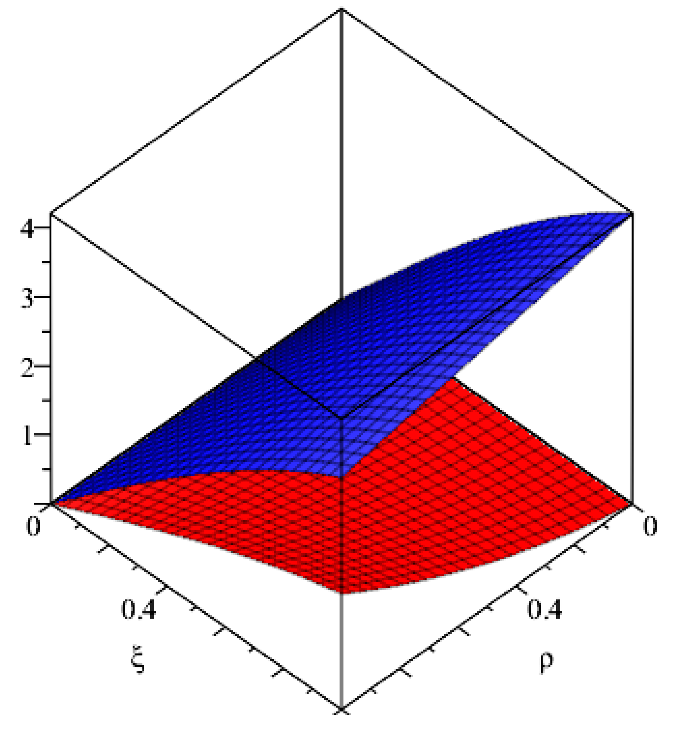
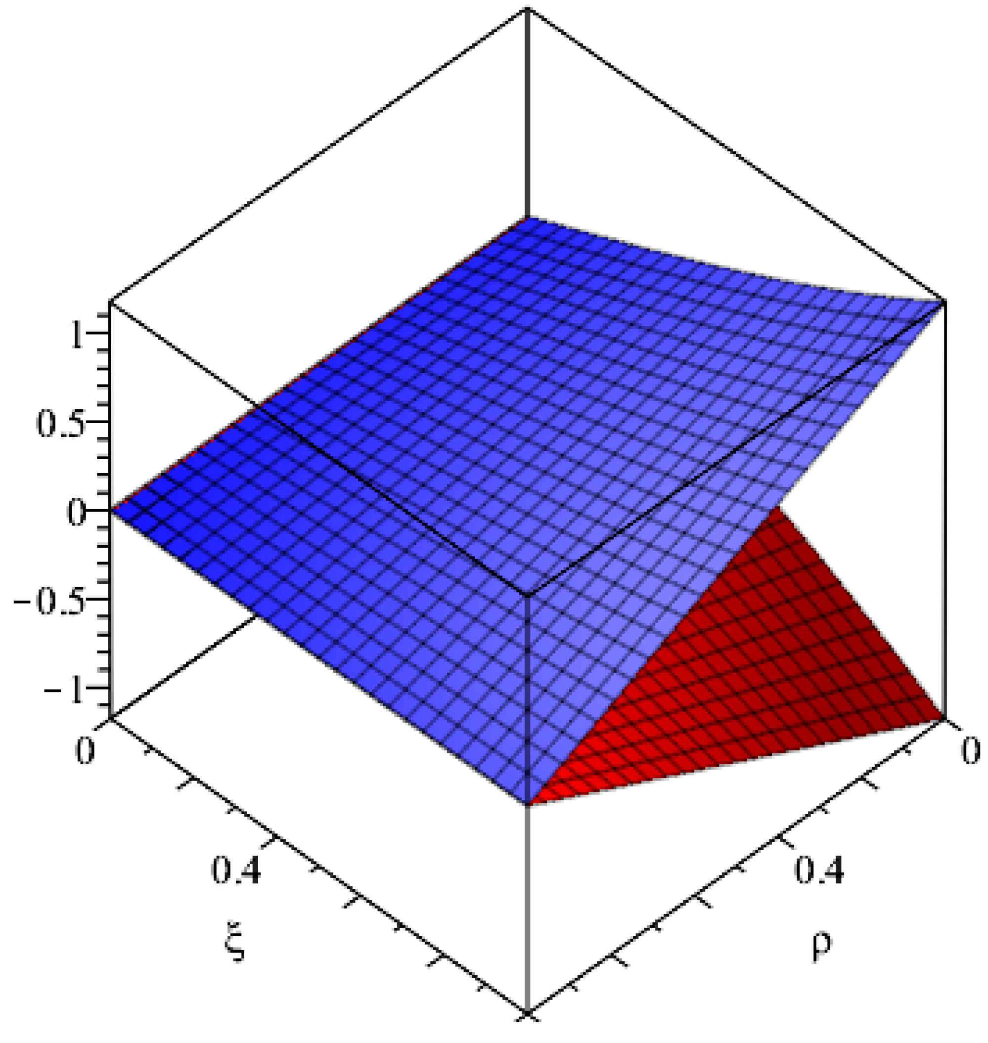
Example 1.

A linear fuzzy integro-differential equation is:

$${{\rm Y}}^{\left(1\right)}\left(\xi ,\rho \right)=f\left(\xi ,\rho \right)-{\displaystyle \underset{0}{\overset{\xi }{\int }}}{\rm Y}\left(t,\rho \right)dt,$$

with conditions,${\rm Y}\left(0,\rho \right)=\left(0,0\right)$, where:

$$\lambda =1,0\le t\le \xi ,0\le \rho \le 1,K\left(\xi ,t\right)=1,$$

i.e.,:

$$f\left(\xi ,\rho \right)=\left(\left({\rho }^2+\rho \right),\left(5-\rho \right)\right)$$

To solve this fuzzy integro-differential, we proceed as follows:

$$\{\begin{array}{c}\underset{\_}{{{\rm Y}}^{\left(1\right)}}\left(\xi ,\rho \right)=f\left(\xi ,\rho \right)-{\displaystyle \underset{0}{\overset{\xi }{\int }}}\underset{\_}{{\rm Y}\left(t,\rho \right)dt}\\ \overline{{{\rm Y}}^{\left(1\right)}}\left(\xi ,\rho \right)=f\left(\xi ,\rho \right)-{\displaystyle \underset{0}{\overset{\xi }{\int }}}\overline{{\rm Y}\left(t,\rho \right)dt}\end{array}$$

(20)

$$\{\begin{array}{c}\underset{\_}{{{\rm Y}}^{\left(1\right)}}\left(\xi ,\rho \right)=\left({\rho }^2+\rho \right)-{\displaystyle \underset{0}{\overset{\xi }{\int }}}\underset{\_}{{\rm Y}\left(t,\rho \right)dt}\\ \overline{{{\rm Y}}^{\left(1\right)}}\left(\xi ,\rho \right)=\left(5-\rho \right)-{\displaystyle \underset{0}{\overset{\xi }{\int }}}\overline{{\rm Y}\left(t,\rho \right)dt}\end{array}$$

(21)

Applying Sumudu transform on (21) and using Equations (A) and (B), we have:

$$\{\begin{array}{c}\mathcal{S}\left[\underset{\_}{{{\rm Y}}^{\left(1\right)}}\left(\xi ,\rho \right)\right]=\mathcal{S}(\left({\rho }^2+\rho \right)-\mathcal{S}{\displaystyle \underset{0}{\overset{\xi }{\int }}}\underset{\_}{{\rm Y}\left(t,\rho \right)dt}\\ \mathcal{S}\overline{[{{\rm Y}}^{\left(1\right)}}\left(\xi ,\rho \right)]=\mathcal{S}(\left(5-\rho \right)-\mathcal{S}{\displaystyle \underset{0}{\overset{\xi }{\int }}}\overline{{\rm Y}\left(t,\rho \right)dt}\end{array}$$

(22)

$$\{\begin{array}{c}\underset{\_}{{\rm Y}}\left(\xi ,\rho \right)={\mathcal{S}}^{-1}\left(u\left({\rho }^2+\rho \right)\right)-{\mathcal{S}}^{-1}(u^2\mathcal{S}\left(\underset{\_}{{\rm Y}}\left(\xi ,\rho \right)\right)\\ \overline{{\rm Y}}\left(\xi ,\rho \right)={\mathcal{S}}^{-1}\left(u\left(5-\rho \right)\right)-{\mathcal{S}}^{-1}(u^2\mathcal{S}\left(\overline{{\rm Y}}\left(\xi ,\rho \right)\right)\end{array}$$

(23)

For$\underset{\_}{{\rm Y}}\left(\xi ,\rho \right)$:

$$\begin{array}{lll}{{\rm Y}}_0=\xi \left({\alpha }^2+\alpha \right)& & \\ {{\rm Y}}_1={\mathcal{S}}^{-1}(u^2\mathcal{S}\left(\xi \left({\rho }^2+\rho \right)\right),& & {{\rm Y}}_1=-\frac{{\xi }^3}{3!}\left({\rho }^2+\rho \right)\\ {{\rm Y}}_2={\mathcal{S}}^{-1}(u^2\mathcal{S}\left(\frac{{\xi }^3}{3!}\left({\rho }^2+\rho \right)\right),& & {{\rm Y}}_2=\frac{{\xi }^5}{5!}\left({\rho }^2+\rho \right)\\ {{\rm Y}}_3={\mathcal{S}}^{-1}(u^2\mathcal{S}\left(\frac{{\xi }^5}{5!}\left({\rho }^2+\rho \right)\right),& & {{\rm Y}}_3=-\frac{{\xi }^7}{7!}\left({\rho }^2+\rho \right)\end{array}$$

Similarly, for$\overline{{\rm Y}\left(\xi ,\rho \right)}$:

$$\begin{array}{lll}{{\rm Y}}_0=\xi \left(5-\rho \right)& & \\ {{\rm Y}}_1={\mathcal{S}}^{-1}(u^2\mathcal{S}\left(\xi \left(5-\rho \right)\right),& & {{\rm Y}}_1=-\frac{{\xi }^3}{3!}\left(5-\rho \right),\\ {{\rm Y}}_2={\mathcal{S}}^{-1}(u^2\mathcal{S}\left(-\frac{{\xi }^3}{3!}\left(5-\rho \right)\right),& & {{\rm Y}}_2=\frac{{\xi }^5}{5!}\left(5-\rho \right),\\ {{\rm Y}}_3={\mathcal{S}}^{-1}(u^2\mathcal{S}\left(\frac{{\xi }^5}{5!}\left(5-\rho \right)\right),& & {{\rm Y}}_3=-\frac{{\xi }^7}{7!}\left(5-\rho \right)\end{array}$$

Thus, using above iterative results, the series form solution is given as:

$$\{\begin{array}{c}\underset{\_}{{\rm Y}\left(\xi ,\rho \right)}=\xi \left(5-\rho \right)-\frac{{\xi }^3}{3!}\left(5-\rho \right)+\frac{{\xi }^5}{5!}\left(5-\rho \right)-\frac{{\xi }^7}{7!}\left(5-\rho \right)+....\\ \overline{{\rm Y}\left(\xi ,\rho \right)}=\xi \left(5-\rho \right)-\frac{{\xi }^3}{3!}\left(5-\rho \right)+\frac{{\xi }^5}{5!}\left(5-\rho \right)-\frac{{\xi }^7}{7!}\left(5-\rho \right)+.....\end{array}$$

(24)

Using (17), we get the exact solution:

$$\{\begin{array}{c}\underset{\_}{{\rm Y}\left(\xi ,\rho \right)}=sin\xi \left({\rho }^2+\rho \right)\\ \overline{{\rm Y}\left(\xi ,\rho \right)}=sin\xi \left(5-\rho \right)\end{array}$$

(25)

A graphical representation of the solution is given in Figure 1.

Figure 1. Graphical interpolation of Example 1.

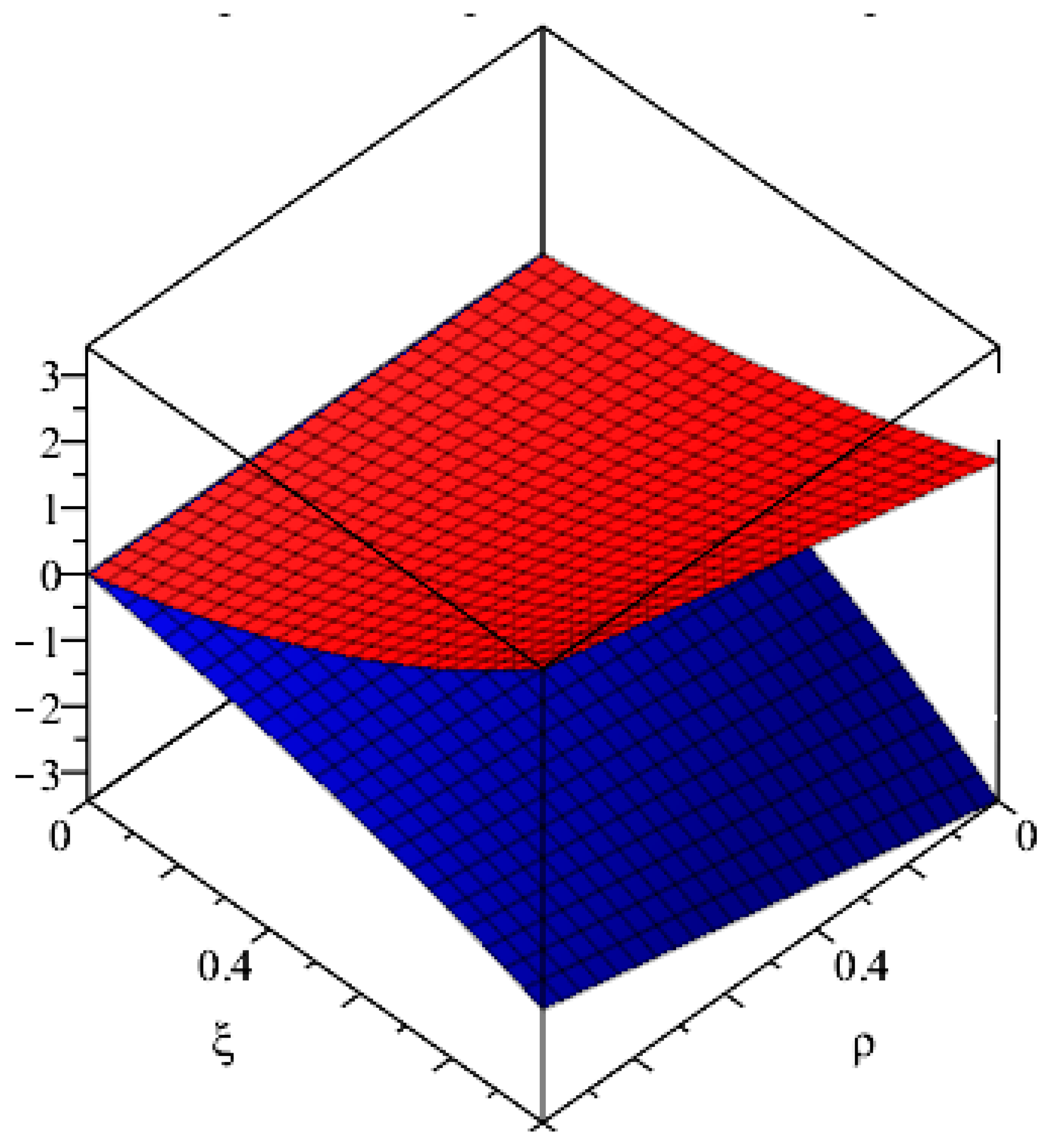
Example 2.

Consider the following fuzzy Volterra integro-differential equation:

$$\begin{array}{c}\{\begin{array}{c}{\underset{\_}{{\rm Y}}}^{\left(1\right)}\left(\xi ,\rho \right)=\left(\rho -1\right)+{\displaystyle \underset{0}{\overset{\xi }{\int }}}\underset{\_}{{\rm Y}}\left(t,\rho \right)dt\\ {\overline{{\rm Y}}}^{\left(1\right)}\left(\xi ,\rho \right)=\left(1-\rho \right)+{\displaystyle \underset{0}{\overset{\xi }{\int }}}\overline{{\rm Y}}\left(t,\rho \right)dt\end{array}\\ {\underset{\_}{{\rm Y}}}^{\left(1\right)}\left(0\right)=0={\overline{{\rm Y}}}^{\left(1\right)}\left(0\right);0\le \rho \le 1,0\le t\le \xi ,\xi \in \left[0,1\right]\end{array}$$

(26)

Using (A) and (B) on both sides and taking the inverse:

$$\{\begin{array}{c}\underset{\_}{{\rm Y}}\left(\xi ,\rho \right))={\mathcal{S}}^{-1}\left(u\left(\rho -1\right)\right)+{\mathcal{S}}^{-1}\left(u^2\mathcal{S}\left[\underset{\_}{{\rm Y}}\left(\xi ,\rho \right)\right]\right)\\ \overline{{\rm Y}}\left(\xi ,\rho \right))={\mathcal{S}}^{-1}\left(u\left(1-\rho \right)\right)+{\mathcal{S}}^{-1}\left(u^2\mathcal{S}\left[\overline{{\rm Y}}\left(\xi ,\rho \right)\right]\right)\end{array}$$

(27)

$$\{\begin{array}{c}\underset{\_}{{\rm Y}}\left(\xi ,\rho \right))=\xi \left(\rho -1\right))+{\mathcal{S}}^{-1}\left(u^2\mathcal{S}\left[\underset{\_}{{\rm Y}}\left(\xi ,\rho \right)\right]\right)\\ \overline{{\rm Y}}\left(\xi ,\rho \right))=\xi \left(1-\rho \right))+{\mathcal{S}}^{-1}\left(u^2\mathcal{S}\left[\overline{{\rm Y}}\left(\xi ,\rho \right)\right]\right)\end{array}$$

Then, the solution in the series form will be:

$${\displaystyle \sum _{i=0}^{\infty }}{\underset{\_}{{\rm Y}}}_i\left(\xi ,\rho \right)={\underset{\_}{{\rm Y}}}_0\left(\xi ,\rho \right)+{\underset{\_}{{\rm Y}}}_1\left(\xi ,\rho \right)+{\underset{\_}{{\rm Y}}}_2\left(\xi ,\rho \right)+{\underset{\_}{{\rm Y}}}_3\left(\xi ,\rho \right)+\cdots$$

$$=\xi \left(\rho -1\right)+\frac{{\xi }^3}{3!}\left(\rho -1\right)+\frac{{\xi }^5}{3!}\left(\rho -1\right)+\frac{{\xi }^7}{3!}\left(\rho -1\right)+\cdots$$

Similarly, for$\overline{{\rm Y}}\left(\xi ,\rho \right)$:

$$=\xi \left(1-\rho \right)+\frac{{\xi }^3}{3!}\left(1-\rho \right)+\frac{{\xi }^5}{5!}\left(1-\rho \right)+\frac{{\xi }^7}{5!}\left(1-\rho \right)+\cdots$$

and the exact solution is given using (17).

$$\overline{{\rm Y}}\left(\xi ,\rho \right)=\left(\rho -1\right)sinht\mathrm{and}\overline{{\rm Y}}\left(\xi ,\rho \right)=\left(1-\rho \right)sinht$$

The graphical representation of the solution is given in Figure 2.

Figure 2. Graphical interpolation of Example 2.

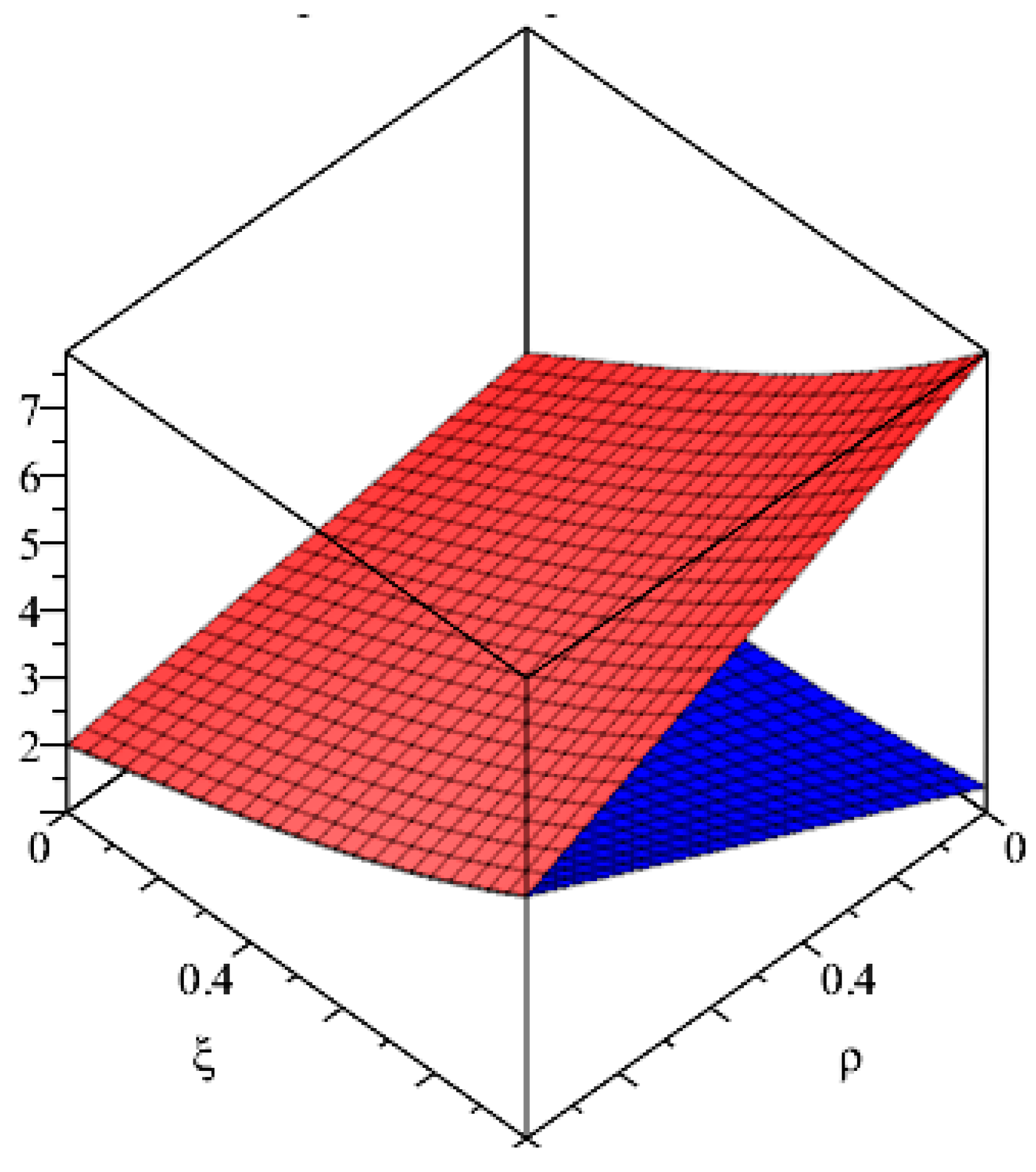
Example 3.

Consider the following fuzzy Volterra integro-differential equation:

$$\begin{array}{c}\{\begin{array}{c}{\underset{\_}{{\rm Y}}}^{\left(1\right)}\left(\xi ,\rho \right)=\left(\rho +1\right)\left(1+\xi \right)+{\displaystyle \underset{0}{\overset{\xi }{\int }}}\underset{\_}{{\rm Y}}\left(t,\rho \right)dt\\ {\overline{{\rm Y}}}^{\left(1\right)}\left(\xi ,\rho \right)=\left(\rho -2\right)\left(1+\xi \right)+{\displaystyle \underset{0}{\overset{\xi }{\int }}}\overline{{\rm Y}}\left(t,\rho \right)dt\end{array}\\ {\underset{\_}{{\rm Y}}}^{\left(1\right)}\left(0\right)=0={\overline{{\rm Y}}}^{\left(1\right)}\left(0\right);0\le \rho \le 1,0\le t\le \xi ,\xi \in \left[0,1\right]\end{array}$$

(28)

Using (A) and (B) on (28), we get:

$$\begin{array}{c}\{\begin{array}{c}\mathcal{S}({\underset{\_}{{\rm Y}}}^{\left(1\right)}\left(\xi ,\rho \right))=\mathcal{S}\left(\left(\rho +1\right)\left(1+\xi \right)\right)+\mathcal{S}[{\displaystyle \underset{0}{\overset{\xi }{\int }}}\underset{\_}{{\rm Y}}\left(t,\rho \right)]dt\\ \mathcal{S}({\overline{{\rm Y}}}^{\left(1\right)}\left(\xi ,\rho \right))=\mathcal{S}\left(\left(\rho -2\right)\left(1+\xi \right)\right)+\mathcal{S}[{\displaystyle \underset{0}{\overset{\xi }{\int }}}\overline{{\rm Y}}\left(t,\rho \right)]dt\end{array}\\ \{\begin{array}{c}\underset{\_}{{\rm Y}}\left(\xi ,\rho \right))={\mathcal{S}}^{-1}\left(u\left(\rho +1\right)\right)+{\mathcal{S}}^{-1}(u^2\left(\rho +1\right)+{\mathcal{S}}^{-1}\left(u^2\mathcal{S}\left[\underset{\_}{{\rm Y}}\left(\xi ,\rho \right)\right]\right)\\ \overline{{\rm Y}}\left(\xi ,\rho \right))={\mathcal{S}}^{-1}\left(u\left(\rho -2\right)\right)+{\mathcal{S}}^{-1}(u^2\left(\rho -2\right)+{\mathcal{S}}^{-1}\left(u^2\mathcal{S}\left[\overline{{\rm Y}}\left(\xi ,\rho \right)\right]\right)\end{array}\end{array}$$

(29)

Then, the solution in the series form will be:

$${\displaystyle \sum _{i=0}^{\infty }}{\underset{\_}{{\rm Y}}}_i\left(\xi ,\rho \right)={\underset{\_}{{\rm Y}}}_0\left(\xi ,\rho \right)+{\underset{\_}{{\rm Y}}}_1\left(\xi ,\rho \right)+{\underset{\_}{{\rm Y}}}_2\left(\xi ,\rho \right)+{\underset{\_}{{\rm Y}}}_3\left(\xi ,\rho \right)+\cdots$$

$$=\xi \left(\rho +1\right)+\frac{{\xi }^2}{2!}\left(\rho +1\right)+\frac{{\xi }^3}{3!}\left(\rho +1\right)+\frac{{\xi }^4}{4!}\left(\rho +1\right)+\frac{{\xi }^5}{5!}\left(\rho +1\right)+\frac{{\xi }^6}{6!}\left(\rho +1\right)\frac{{\xi }^7}{7!}\left(\rho +1\right)+\frac{{\xi }^8}{8!}\left(\rho +1\right)+\cdots$$

(30)

Similarly, for$\overline{{\rm Y}}\left(\xi ,\rho \right)$:

$$=\xi \left(\rho -2\right)+\frac{{\xi }^2}{2!}\left(\rho -2\right)+\frac{{\xi }^3}{3!}\left(\rho -2\right)+\frac{{\xi }^4}{4!}\left(\rho -2\right)+\frac{{\xi }^5}{5!}\left(\rho -2\right)+\frac{{\xi }^6}{6!}\left(\rho -2\right)\frac{{\xi }^7}{7!}\left(\rho -2\right)+\frac{{\xi }^8}{8!}\left(\rho -2\right)+\cdots$$

(31)

Using (17), we get the exact solution.

$$\underset{\_}{{\rm Y}}\left(\xi ,\rho \right)=\left(\rho +1\right)\left(e^x-1\right)\mathrm{and}\overline{{\rm Y}}\left(\xi ,\rho \right)=\left(\rho -2\right)\left(e^x-1\right)$$

The graphical representation of the solution is given in Figure 3.

Figure 3. Graphical interpretation of Example 3.

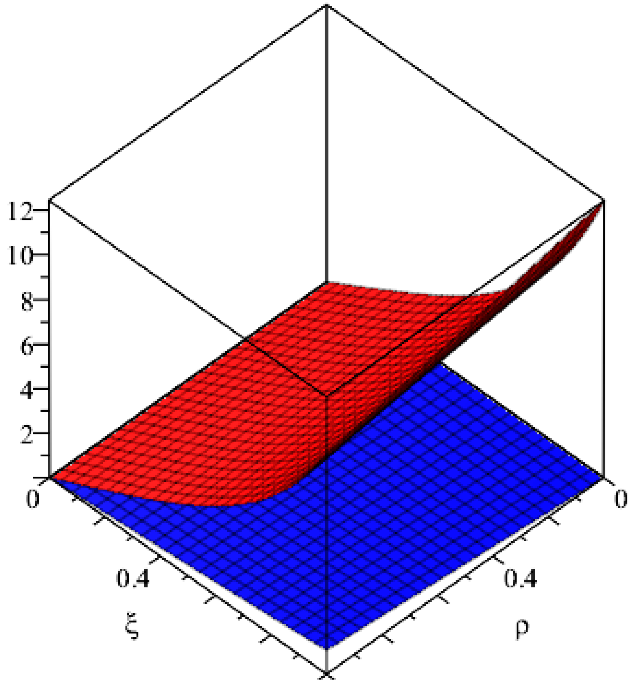
Example 4.

Consider a Volterra integro-differential equation:

$${{\rm Y}}^{\left(2\right)}\left(\xi ,\rho \right)=f\left(\xi ,\rho \right)-{\displaystyle \underset{0}{\overset{\xi }{\int }}}\left(\xi -t\right){\rm Y}\left(t,\rho \right)dt$$

(32)

with conditions:

$$\begin{array}{c}u\left(0,\rho \right)=\left(\rho +1,3-\rho \right);u^{\left(1\right)}\left(0,\rho \right)=\left(\rho ,2-\rho \right)\\ \lambda =1,0\le t\le \xi ,0\le \rho \le 1,K\left(\xi ,t\right)=\left(\xi -t\right),\end{array}$$

To solve Equation (32), we proceed as follows:

$$\{\begin{array}{c}\underset{\_}{u^{\left(2\right)}\left(\xi ,\rho \right)}=f\left(\xi ,\rho \right)-{\displaystyle \underset{0}{\overset{\xi }{\int }}}\left(\xi -t\right)\underset{\_}{{\rm Y}\left(t,\rho \right)dt}\\ \overline{u^{\left(2\right)}\left(\xi ,\rho \right)}=f\left(\xi ,\rho \right)-{\displaystyle \underset{0}{\overset{\xi }{\int }}}\left(\xi -t\right)\overline{{\rm Y}\left(t,\rho \right)dt}\end{array}$$

(33)

$$\{\begin{array}{c}\underset{\_}{u^{\left(2\right)}\left(\xi ,\rho \right)}=\left(\rho +2\right)\xi -{\displaystyle \underset{0}{\overset{\xi }{\int }}}\left(\xi -t\right)\underset{\_}{{\rm Y}\left(t,\rho \right)dt}\\ \overline{u^{\left(2\right)}\left(\xi ,\alpha \right)}=\left(4-\rho \right)\xi -{\displaystyle \underset{0}{\overset{\xi }{\int }}}\left(\xi -t\right)\overline{{\rm Y}\left(t,\rho \right)dt}\end{array}$$

(34)

Using (A) and (B), we get:

$$\{\begin{array}{c}\underset{\_}{{\rm Y}\left(\xi ,\rho \right)}={\mathcal{S}}^{-1}(u^3\left(\rho +2\right)+{\mathcal{S}}^{-1}\left(u\rho \right)+{\mathcal{S}}^{-1}\left(\rho +1\right)-{\mathcal{S}}^{-1}(u^4\mathcal{S}\left(\underset{\_}{{\rm Y}\left(\xi ,\rho \right)}\right)\\ \overline{{\rm Y}\left(\xi ,\rho \right)}={\mathcal{S}}^{-1}(u^3\left(4-\rho \right)+{\mathcal{S}}^{-1}\left(2-\rho \right)+{\mathcal{S}}^{-1}\left(3-\rho \right)-{\mathcal{S}}^{-1}(u^4\mathcal{S}\left(\overline{{\rm Y}\left(\xi ,\rho \right)}\right)\end{array}$$

(35)

Now, applying the decomposition method for$\underset{\_}{{\rm Y}\left(\xi ,\rho \right)}$:

$$\begin{array}{lll}{{\rm Y}}_0=\frac{{\xi }^3}{3!}\left(\rho +2\right)+\xi \rho +\left(\rho +1\right)& & \\ {{\rm Y}}_1={\mathcal{S}}^{-1}\left(u^4\mathcal{S}\left(\frac{{\xi }^3}{3!}\left(\rho +2\right)+\xi \rho +\left(\rho +1\right)\right)\right),& & {{\rm Y}}_1=\frac{{\xi }^7}{7!}\left(\rho +2\right)+\frac{{\xi }^5}{5!}\rho +\frac{{\xi }^4}{4!}\left(\rho +1\right)\\ {{\rm Y}}_2={\mathcal{S}}^{-1}\left(u^4\mathcal{S}(\frac{{\xi }^7}{7!}\left(\rho +2\right)+\frac{{\xi }^5}{5!}\rho +\frac{{\xi }^4}{4!}\left(\rho +1\right)\right)& & {{\rm Y}}_2=\frac{{\xi }^{11}}{11!}\left(\rho +2\right)+\frac{{\xi }^9}{9!}\rho +\frac{{\xi }^8}{8!}\left(\rho +1\right)\end{array}$$

Similarly, we can find$\underset{\_}{{{\rm Y}}_3}\left(\xi ,\rho \right),\underset{\_}{{{\rm Y}}_4}\left(\xi ,\rho \right),....$:

$$\begin{array}{cc}\hfill {\displaystyle \sum _{i=0}^{\infty }}\underset{\_}{{{\rm Y}}_i}\left(\xi ,\rho \right)& =\underset{\_}{{{\rm Y}}_0}\left(\xi ,\rho \right)+\underset{\_}{{{\rm Y}}_1}\left(\xi ,\rho \right)+\underset{\_}{{{\rm Y}}_2}\left(\xi ,\rho \right)+....\hfill \\ & =\left(\xi +\frac{{\xi }^5}{5!}+\frac{{\xi }^9}{9!}+.....\right)\rho +\left(1+\frac{{\xi }^4}{4!}+\frac{{\xi }^8}{8!}+.....\right)\left(\rho +1\right)\hfill \\ & +\left(\frac{{\xi }^3}{3!}+\frac{{\xi }^7}{7!}+\frac{{\xi }^{11}}{11!}.....\right)\left(\rho +2\right)+\cdots \hfill \end{array}$$

(36)

Now, for$\overline{{\rm Y}\left(\xi ,\rho \right)}$:

$$\begin{array}{c}{{\rm Y}}_0=\frac{{\xi }^3}{3!}\left(4-\rho \right)+\xi \left(2-\rho \right)+\left(3-\rho \right)\\ {{\rm Y}}_1={\mathcal{S}}^{-1}(u^4\mathcal{S}\left(\frac{\xi }{3!}\left(4-\rho \right)+\xi \left(2-\rho \right)+\left(3-\rho \right)\right),\\ \\ {{\rm Y}}_1=\frac{{\xi }^7}{7!}\left(4-\rho \right)+\frac{{\xi }^5}{5!}\left(2-\rho \right)+\frac{{\xi }^4}{4!}\left(3-\rho \right)\\ {{\rm Y}}_2={\mathcal{S}}^{-1}(u^4\mathcal{S}\left(\frac{{\xi }^7}{7!}\left(4-\rho \right)+\frac{{\xi }^5}{5!}\left(2-\rho \right)+\frac{{\xi }^4}{4!}\left(3-\rho \right)\right),\\ {{\rm Y}}_2=\frac{{\xi }^{11}}{11!}\left(4-\rho \right)+\frac{{\xi }^9}{9!}\left(2-\rho \right)+\frac{{\xi }^8}{8!}\left(3-\rho \right)\end{array}$$

Similarly, for$\overline{{{\rm Y}}_i}\left(\xi ,\rho \right)$:

$$\begin{array}{l}=\left(\xi +\frac{{\xi }^5}{5!}+\frac{{\xi }^9}{9!}+.....\right)\left(2-\rho \right)+\left(1+\frac{{\xi }^4}{4!}+\frac{{\xi }^8}{8!}+.....\right)\left(3-\rho \right)\\ +\left(\frac{{\xi }^3}{3!}+\frac{{\xi }^7}{7!}+\frac{{\xi }^{11}}{11!}.....\right)\left(4-\rho \right)+\cdots \end{array}$$

and the exact solution is given as:

$$\begin{array}{c}\underset{\_}{{\rm Y}}\left(\xi ;\rho \right)=\left(\rho +2\right).\frac{1}{2}\left(sinh\xi -sin\xi \right)+\left(\rho +1\right).\frac{1}{2}\left(cos\xi +cosh\xi \right)+\left(\rho \right)\left(sin\xi +sinh\xi \right)\\ \\ \overline{{\rm Y}}\left(t;\rho \right)=\left(4-\rho \right).\frac{1}{2}\left(sinh\xi -sin\xi \right)+\left(3-\rho \right).\frac{1}{2}\left(cos\xi +cosh\xi \right)\\ +\left(2-\rho \right)\left(sin\xi +sinh\xi \right)0\le \rho \le 1\end{array}$$

The graphical representation of the solution is given in Figure 4.

Figure 4. Graphical interpretation of Example 4.

Example 5.

Consider a nonlinear fuzzy Volterra integro-differential equation:

$${{\rm Y}}^{\left(1\right)}\left(\xi ,\rho \right)=f\left(\xi ,\rho \right)-{\displaystyle \underset{0}{\overset{\xi }{\int }}}{{\rm Y}}^2\left(t,\rho \right)dt$$

(37)

with conditions${\rm Y}\left(0,\rho \right)=\left(0,0\right)$, where:

$$\begin{array}{c}\lambda =1,0\le t\le \xi ,0\le \rho \le 1,K\left(\xi ,t\right)=1,\mathrm{i}.\mathrm{e}.,\\ f\left(\xi ,\rho \right)=\left(\rho ,7-\rho \right)\end{array}$$

To solve Equation (37), we proceed as follows:

$$\{\begin{array}{c}\underset{\_}{{{\rm Y}}^{\left(1\right)}\left(\xi ,\rho \right)}=f\left(\xi ,\rho \right)-{\displaystyle \underset{0}{\overset{\xi }{\int }}}\underset{\_}{{{\rm Y}}^2\left(t,\rho \right)dt}\\ \overline{{{\rm Y}}^{\left(1\right)}\left(\xi ,\rho \right)}=f\left(\xi ,\rho \right)-{\displaystyle \underset{0}{\overset{\xi }{\int }}}\overline{{{\rm Y}}^2\left(t,\rho \right)dt}\end{array}$$

(38)

$$\{\begin{array}{c}\underset{\_}{{{\rm Y}}^{\left(1\right)}\left(\xi ,\rho \right)}=\rho -{\displaystyle \underset{0}{\overset{\xi }{\int }}}\underset{\_}{{{\rm Y}}^2\left(t,\rho \right)dt}\\ \overline{{{\rm Y}}^{\left(1\right)}\left(\xi ,\rho \right)}=7-\rho -{\displaystyle \underset{0}{\overset{\xi }{\int }}}\overline{{{\rm Y}}^2\left(t,\rho \right)dt}\end{array}$$

(39)

Applying the Sumudu transform on both sides of the equation, we get:

$$\{\begin{array}{c}\mathcal{S}(\underset{\_}{{{\rm Y}}^{\left(1\right)}\left(\xi ,\rho \right)}=\mathcal{S}\left(\rho \right)-\mathcal{S}{\displaystyle \underset{0}{\overset{\xi }{\int }}}\underset{\_}{{{\rm Y}}^2\left(t,\rho \right)dt}\\ \mathcal{S}(\overline{{{\rm Y}}^{\left(1\right)}\left(\xi ,\rho \right)}=\mathcal{S}\left(7-\rho \right)-\mathcal{S}{\displaystyle \underset{0}{\overset{\xi }{\int }}}\overline{{{\rm Y}}^2\left(t,\rho \right)dt}\end{array}$$

(40)

Applying the inverse Sumudu transform and using (19), we get:

$$\{\begin{array}{c}\underset{\_}{{\rm Y}\left(\xi ,\rho \right)}={\mathcal{S}}^{-1}\left(u\rho \right)-{\mathcal{S}}^{-1}(u^2\mathcal{S}\left({{\rm Y}}^2\underset{\_}{\left(\xi ,\rho \right)}\right)\\ \overline{{\rm Y}\left(\xi ,\rho \right)}={\mathcal{S}}^{-1}\left(u\left(7-\rho \right)\right)-{\mathcal{S}}^{-1}(u^2\mathcal{S}\left(\overline{{{\rm Y}}^2\left(\xi ,\rho \right)}\right)\end{array}$$

$$\begin{array}{cc}\hfill {\displaystyle \sum _{i=0}^{\infty }}\overline{{{\rm Y}}_i}\left(\xi ,\rho \right)& =\overline{{{\rm Y}}_1}\left(\xi ,\rho \right)+\overline{{{\rm Y}}_2}\left(\xi ,\rho \right)+\overline{{{\rm Y}}_3}\left(\xi ,\rho \right)+....\hfill \\ & =\xi \left(7-\rho \right)+\frac{{\xi }^4}{12}{\left(7-\rho \right)}^2+\frac{{\xi }^7}{252}{\left(7-\rho \right)}^3+\dots \hfill \end{array}$$

The graphical representation of the solution is given in Figure 5.

Figure 5. Graphical interpretation of Example 5.

6. Conclusions

Usually, it is difficult to solve fuzzy integro-differential equations analytically. Most probably, it is required to obtain the approximate solutions. In this paper, we developed a numerical technique (Sumudu decomposition method) to find the solution to linear and nonlinear fuzzy Volterra integro-differential equations. A general method for solving VIDE was developed. This technique proved reliable and effective based on the achieved results. It gives fast convergence because by utilizing a lower number of iterations, we get approximate as well as exact solutions.