An Alternative to Real Number Axioms


Abstract
:1. Introduction
2. Materials and Methods
- 1.
- F is non-decreasing
- 2.
- F is right continuous in any point,
- 3.
- 4.
- .
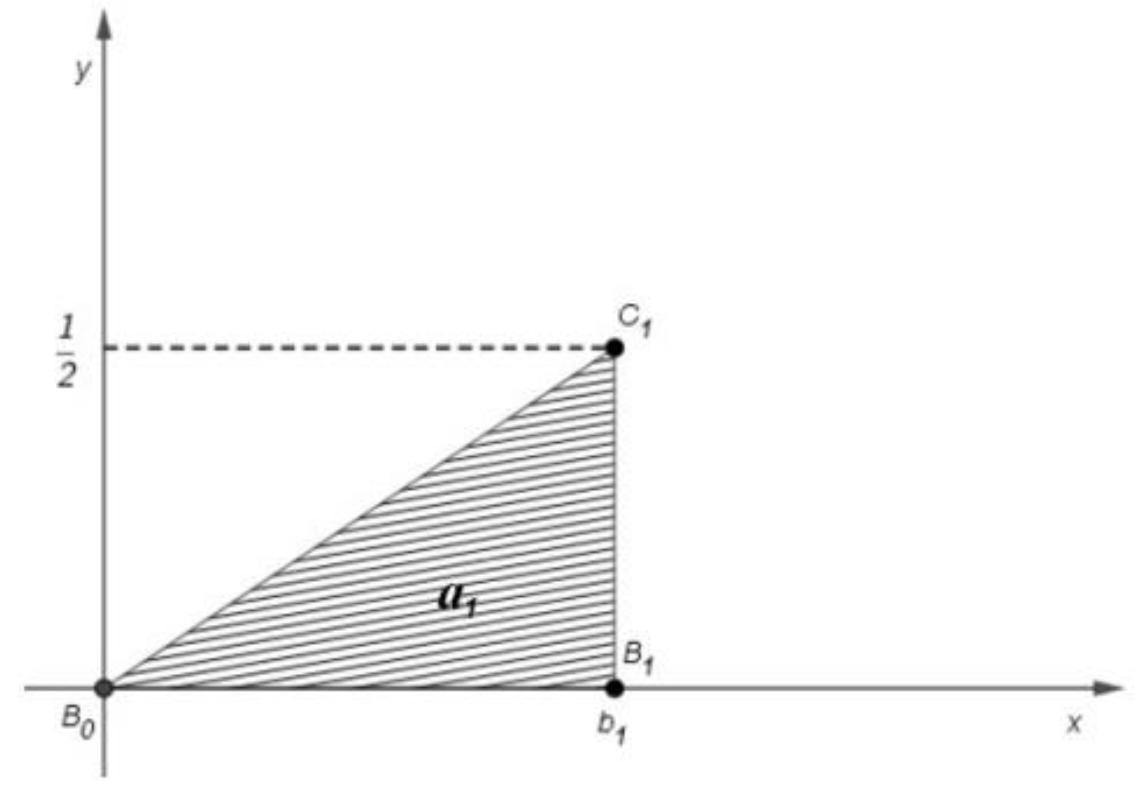
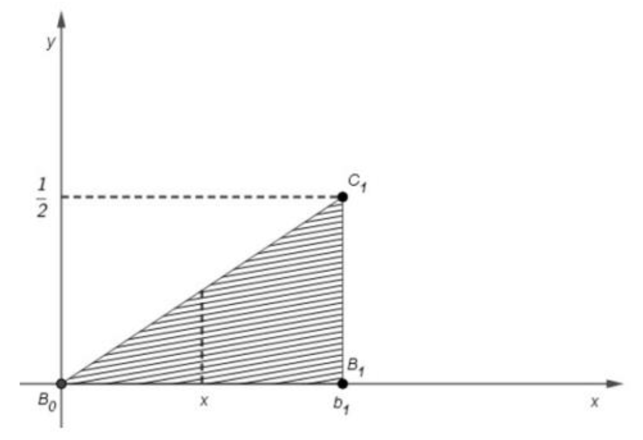
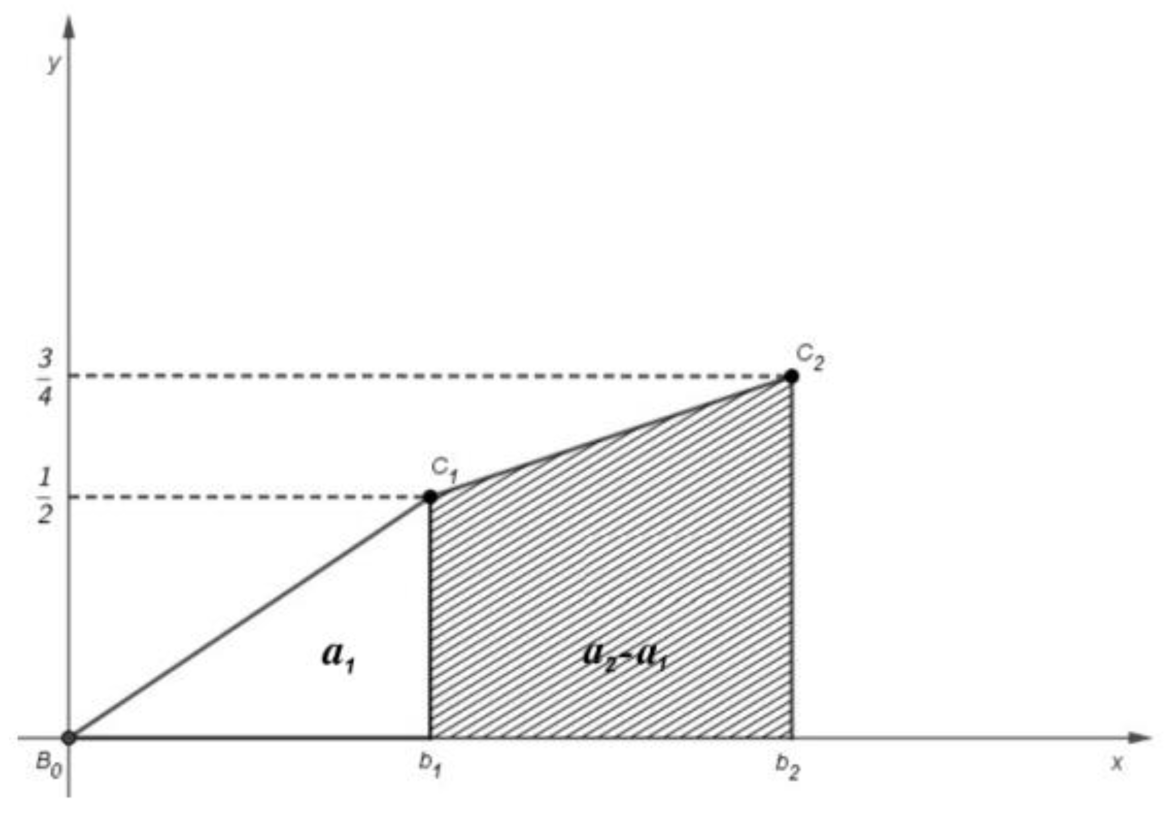
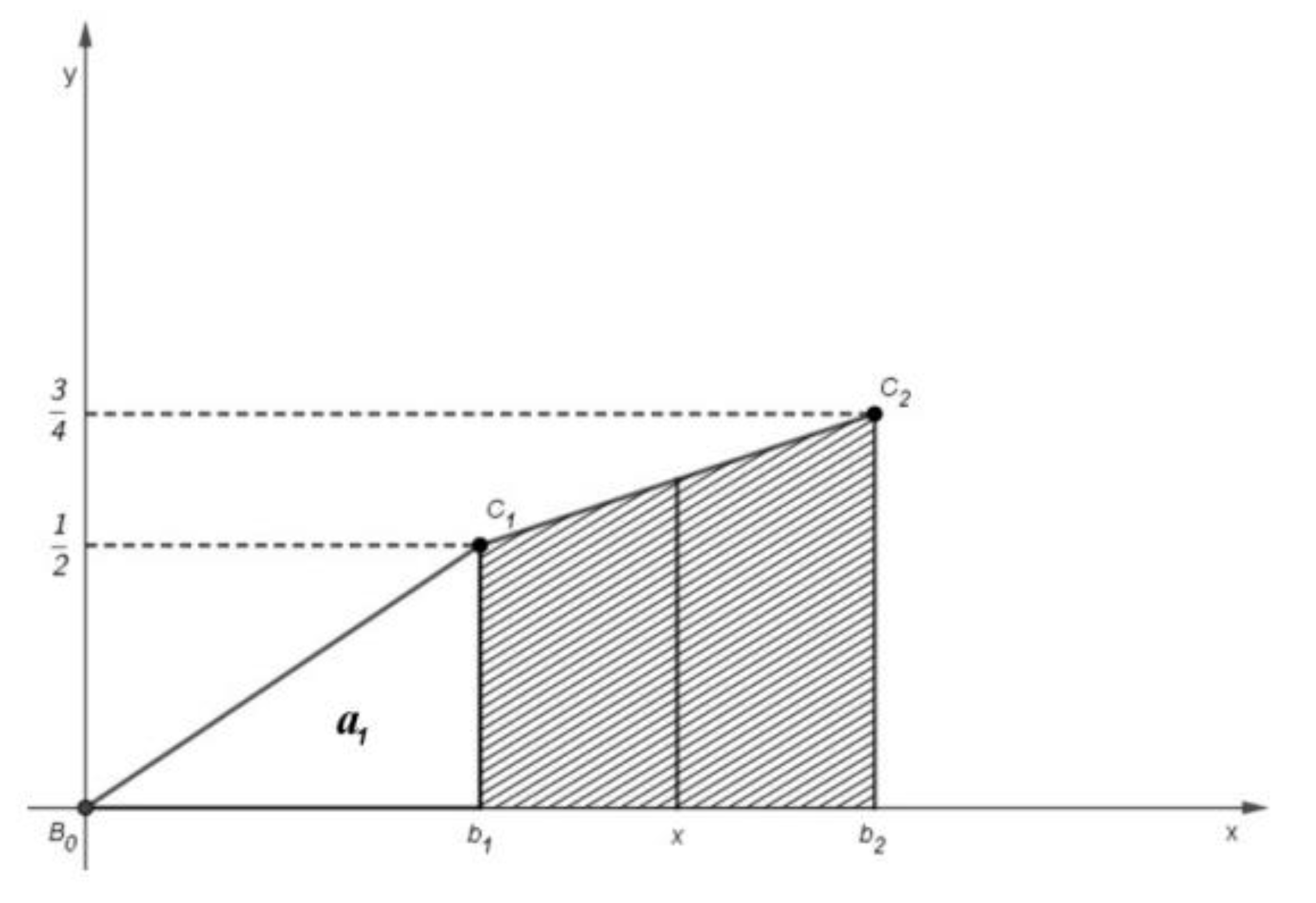
3. Results
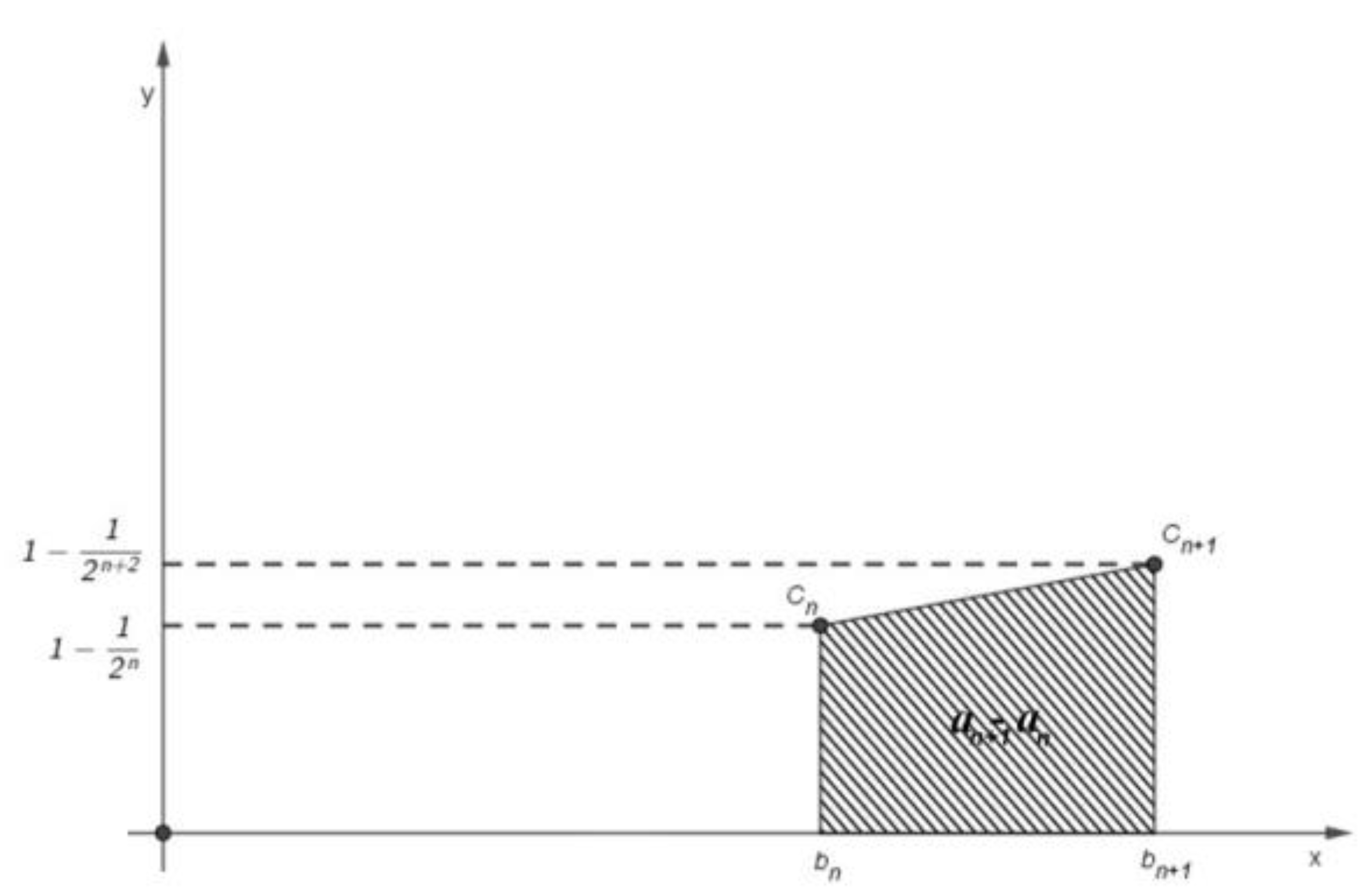
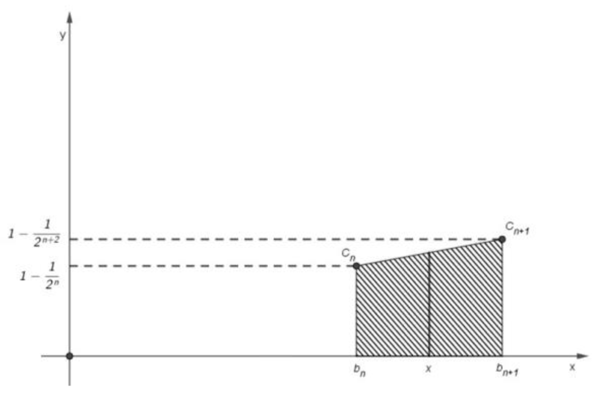
- For all , put .
- If there exists a natural number n and , then
- if for all natural numbers n, then .
4. Conclusions
Author Contributions
Funding
Acknowledgments
Conflicts of Interest
References
- Teissman, H. Toward a More Complete List of Completeness Axiom. Am. Math. Mon. 2013, 120, 99–114. [Google Scholar] [CrossRef]
- Riečan, B.; Neubrunn, T. Integral, Measure and Ordening; Springer Science & Business Media: Berlin/Heidelberg, Germany, 2013. [Google Scholar]
- Billingsley, P. Probability and Measure; John Wiley & Sons: Hoboken, NJ, USA, 2008. [Google Scholar]


© 2018 by the authors. Licensee MDPI, Basel, Switzerland. This article is an open access article distributed under the terms and conditions of the Creative Commons Attribution (CC BY) license (http://creativecommons.org/licenses/by/4.0/).
Share and Cite
Líška, I.; Riečan, B.; Tirpáková, A. An Alternative to Real Number Axioms. Axioms 2018, 7, 59. https://doi.org/10.3390/axioms7030059
Líška I, Riečan B, Tirpáková A. An Alternative to Real Number Axioms. Axioms. 2018; 7(3):59. https://doi.org/10.3390/axioms7030059
Chicago/Turabian StyleLíška, Igor, Beloslav Riečan, and Anna Tirpáková. 2018. "An Alternative to Real Number Axioms" Axioms 7, no. 3: 59. https://doi.org/10.3390/axioms7030059
APA StyleLíška, I., Riečan, B., & Tirpáková, A. (2018). An Alternative to Real Number Axioms. Axioms, 7(3), 59. https://doi.org/10.3390/axioms7030059