Certain Notions of Energy in Single-Valued Neutrosophic Graphs

Abstract

A single-valued neutrosophic set is an instance of a neutrosophic set, which provides us an additional possibility to represent uncertainty, imprecise, incomplete and inconsistent information existing in real situations. In this research study, we present concepts of energy, Laplacian energy and signless Laplacian energy in single-valued neutrosophic graphs (SVNGs), describe some of their properties and develop relationship among them. We also consider practical examples to illustrate the applicability of the our proposed concepts.

1. Introduction

Smarandache [1] originally introduced the notion of neutrosophic set (NS) from philosophical point of view. Wang et al. [2] put forth the notion of a single-valued neutrosophic set (SVNS) from a scientific or engineering point of view, as a subclass of the NS and an extension of intuitionistic fuzzy set (IFS) [3], and provide its various properties. The prominent characteristic of SVNS is that a truth-membership, an indeterminacy-membership and a falsity-membership degree, in [0,1] are independently assigned to each element in the set. IFSs cannot deal with all types of uncertainty, such as indeterminate and inconsistent information, existing commonly in real situations. For instance, if during a voting process there are sixteen voters, seven vote ‘aye’, six vote ‘blackball’ and three are undecided. According to single-valued neutrosophic notation, it can be represented as $u\langle 0.7,0.3,0.6\rangle$. This information is beyond the scope of IFS. That is why, the concept of SVNS is more extensive than IFS. NS, particularly SVNS has attracted significant interest from researchers in recent years. It has been widely applied in various fields, including information fusion in which data are combined from different sensors [4], control theory [5], image processing [6], medical diagnosis [7], decision making [8], and graph theory [9,10].

A graph is a mathematical object containing points (vertices) and connections (edges). For instance, the vertices could represent communication centers, with edges depicting communication links. Graph spectra is one of the most important concepts of graph theory. Gutman [11] introduced the notion of energy of a graph in chemistry, because of its relevance to the total $\pi$-electron energy of certain molecules and found upper and lower bounds for the energy of graphs [12]. Later, Gutman and Zhou [13] defined the Laplacian energy of a graph as the sum of the absolute values of the differences of average vertex degree of G to the Laplacian eigenvalues of G. Signless Laplacian energy of a graph was defined in [14]. However, in many real-life applications, there is a variety of non-deterministic information due to the increase of system complexity. Sometimes, the connection between two objects cannot be fully determined and to verify the properties of the graph traditional methods are useless. Erdös [15] used the probability theory, to deal with this problem. Meanwhile, after the inception of fuzzy sets by Zadeh [16], the concept of fuzzy graph was put forth by Kaufmann [17] and Rosenfeld [18] to handle the fuzzy phenomena in graphs. Fuzzy graphs are useful in representing structures of relationships between objects, where the existence of a concrete object and relationship between two objects are uncertain or obscure. Anjali and Mathew [19] investigated the energy of a graph within the framework of fuzzy set theory. Laplacian energy of a fuzzy graph was defined by Sharbaf and Fayazi [20]. Later on, many generalized fuzzy graphs [21,22,23,24,25,26,27,28,29,30,31] have been introduced in literature. Among these extensions, the notion of intuitionistic fuzzy graph (IFG) whose vertex set and edge set specify a degree of membership, a degree of non-membership and a degree of hesitancy was proposed by Parvathi and Karunambigai [21], and Akram and Davvaz [23]. Praba et al. [32] defined the energy of IFGs. Basha and Kartheek [33] generalized the concept of the Laplacian energy of fuzzy graph to the Laplacian energy of an IFG. When description of the objects or their relations or both is indeterminate and inconsistent, it cannot be handled by fuzzy graphs and IFGs. To overcome this shortcoming of the IFGs, Akram et al. [24] extended the concept of IFGs to SVNGs and put forward many new concepts related to SVNGs and its extensions [24,25,26]. Naz et al. [10] introduced the concept of single-valued neutrosophic digraphs (SVNDGs). In this research study, we present concepts of energy, Laplacian energy and signless Laplacian energy in single-valued neutrosophic graphs (SVNGs), describe some of their properties and develop relationship among them. We also consider practical examples to illustrate the applicability of the our proposed concepts.

Definition 1.

[2] Let Z be a space of points (objects), with a generic element in Z denoted by u. A SVNS X in Z is characterized by a truth-membership function $T_X$, an indeterminacy-membership function $I_X$ and a falsity-membership function $F_X$. For each point $u\in X$, $T_X(u),I_X(u),F_X(u)\in [0,1]$. Therefore, a SVNS X in Z can be written as

$$X=\{\langle u,T_X(u),I_X(u),F_X(u)\rangle |u\in Z\}.$$

Definition 2.

[24] A SVNG on a non-empty set Z is a pair $\mathcal{G}=(X,Y)$, where X is a single-valued neutrosophic set (SVNS) in Z and Y is a single-valued neutrosophic relation on Z such that

$$T_Y(uv)\le min\{T_X(u),T_X(v)\},$$

$$I_Y(uv)\le max\{I_X(u),I_X(v)\},$$

$$F_Y(uv)\le max\{F_X(u),F_X(v)\}$$

for all $u,v\in Z$. X and Y are called the single-valued neutrosophic vertex set and the single-valued neutrosophic edge set of $\mathcal{G}$, respectively. Here Y is a symmetric single-valued neutrosophic relation on X. If Y is not symmetric on X, then $\mathcal{D}=(X,\overrightarrow{Y})$ is called SVNDG.

We have used standard definitions and terminologies, in this paper. For more details and background, the readers are referred to [34,35,36,37,38,39,40].

2. Energy of Single-Valued Neutrosophic Graphs

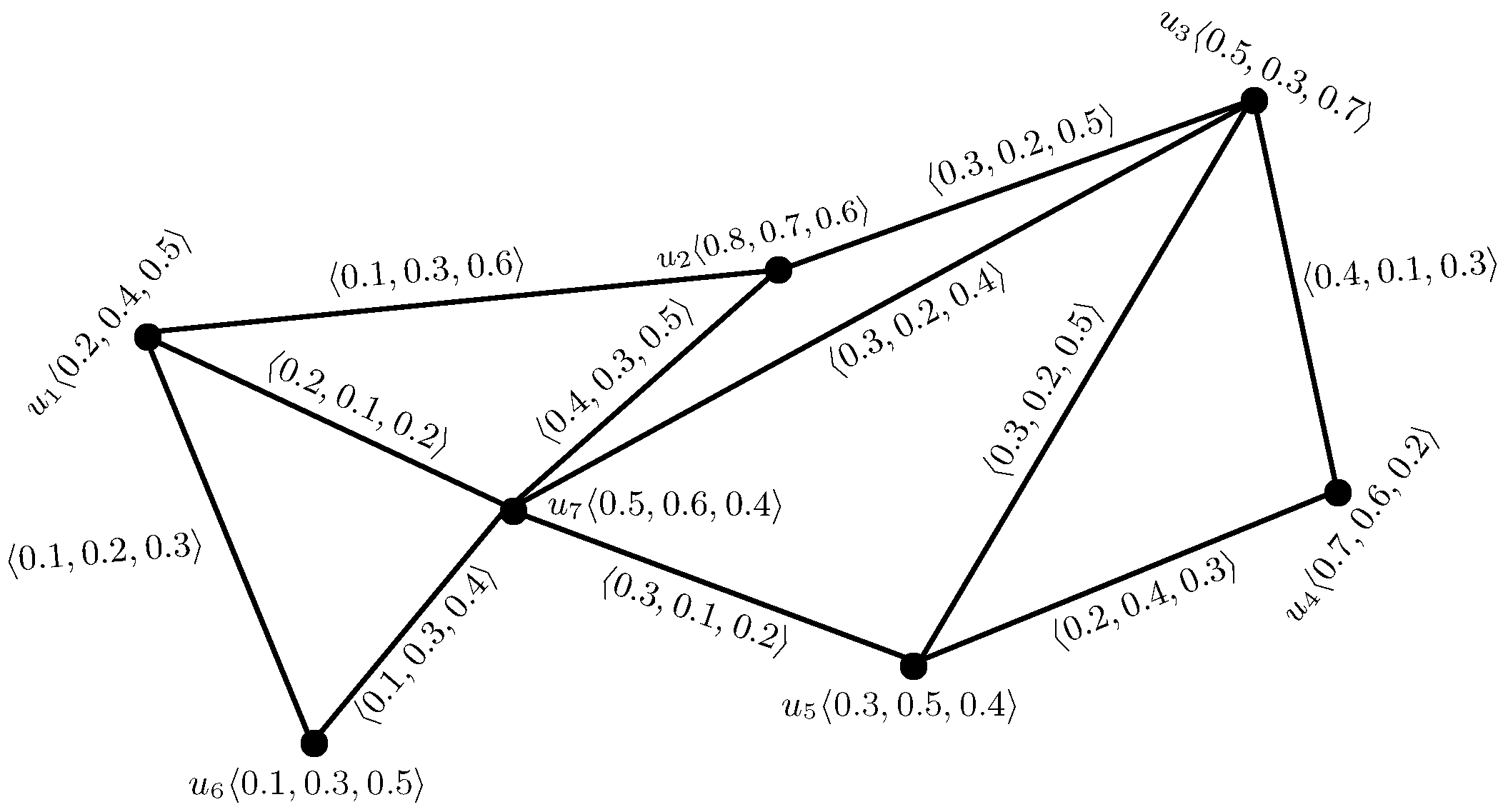
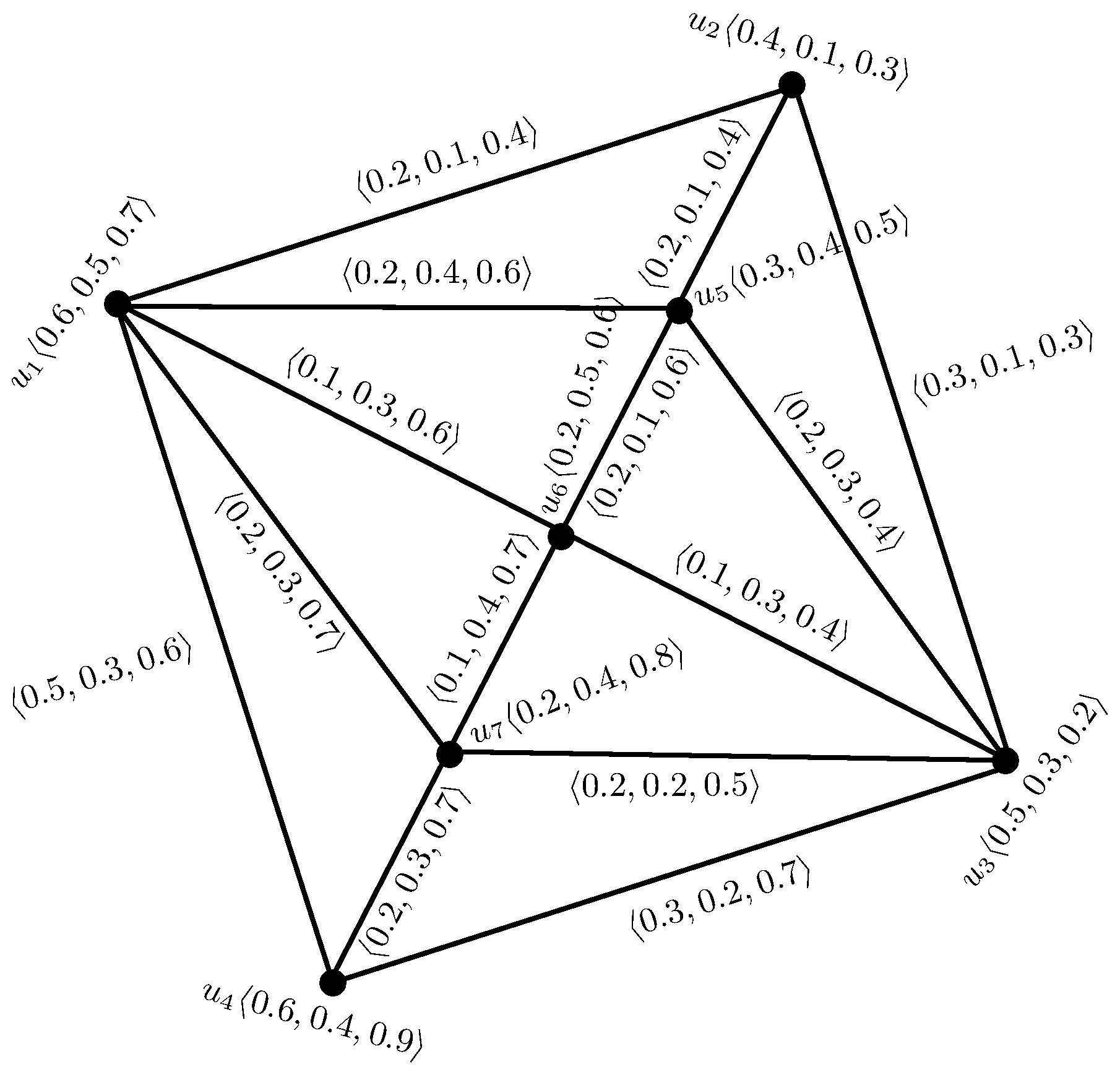
In this section, we define and investigate the energy of a graph within the framework of SVNS theory and discuss its properties.

Definition 3.

The adjacency matrix $A(\mathcal{G})$ of a SVNG $\mathcal{G}=(X,Y)$ is defined as a square matrix $A(\mathcal{G})=\left[a_{jk}\right],$ $a_{jk}=\langle T_Y(u_j{u}_k),I_Y(u_j{u}_k),F_Y(u_j{u}_k)\rangle$, where $T_Y(u_j{u}_k),I_Y(u_j{u}_k)$ and $F_Y(u_j{u}_k)$ represent the strength of relationship, strength of undecided relationship and strength of non-relationship between $u_j$ and $u_k$, respectively.

The adjacency matrix of a SVNG can be expressed as three matrices, first matrix contains the entries as truth-membership values, second contains the entries as indeterminacy-membership values and the third contains the entries as falsity-membership values, i.e., $A(\mathcal{G})=\langle A(T_Y(u_j{u}_k)),A(I_Y(u_j{u}_k)),A(F_Y(u_j{u}_k))\rangle$.

Definition 4.

The spectrum of adjacency matrix of a SVNG $A(\mathcal{G})$ is defined as $\langle M,N,O\rangle$, where M, N and O are the sets of eigenvalues of $A(T_Y(u_j{u}_k))$, $A(I_Y(u_j{u}_k))$ and $A(F_Y(u_j{u}_k))$, respectively.

Example 1.

Consider a graph $G=(V,E)$, where $V=\{u_1,u_2,u_3,u_4,u_5,u_6,u_7\}$ and $E=\{u_1{u}_2,u_2{u}_3,u_3{u}_4,u_4{u}_1,u_1{u}_5,u_1{u}_6,u_1{u}_7,u_3{u}_5,u_3{u}_6,u_3{u}_7,u_2{u}_5,u_5{u}_6,u_6{u}_7,u_4{u}_7\}$. Let $\mathcal{G}=(X,Y)$ be a SVNG on V, as shown in Figure 1, defined by

X	u1	u2	u3	u4	u5	u6	u7
$T_X$	0.6	0.4	0.5	0.6	0.3	0.2	0.2
$I_X$	0.5	0.1	0.3	0.4	0.4	0.5	0.4
$F_X$	0.7	0.3	0.2	0.9	0.5	0.6	0.8

Y	u1u2	u2u3	u3u4	u4u1	u1u5	u1u6	u1u7	u3u5	u3u6	u3u7	u2u5	u5u6	u6u7	u4u7
$T_Y$	0.2	0.3	0.3	0.5	0.2	0.1	0.2	0.2	0.1	0.2	0.2	0.2	0.1	0.2
$I_Y$	0.1	0.1	0.2	0.3	0.4	0.3	0.3	0.3	0.3	0.2	0.1	0.1	0.4	0.3
$F_Y$	0.4	0.3	0.7	0.6	0.6	0.6	0.7	0.4	0.4	0.5	0.4	0.6	0.7	0.7

The adjacency matrix of a SVNG given in Figure 1, is

$$A(\mathcal{G})=\left(\begin{array}{ccccccc}\langle 0,0,0\rangle & \langle 0.2,0.1,0.4\rangle & \langle 0,0,0\rangle & \langle 0.5,0.3,0.6\rangle & \langle 0.2,0.4,0.6\rangle & \langle 0.1,0.3,0.6\rangle & \langle 0.2,0.3,0.7\rangle \\ \langle 0.2,0.1,0.4\rangle & \langle 0,0,0\rangle & \langle 0.3,0.1,0.3\rangle & \langle 0,0,0\rangle & \langle 0.2,0.1,0.4\rangle & \langle 0,0,0\rangle & \langle 0,0,0\rangle \\ \langle 0,0,0\rangle & \langle 0.3,0.1,0.3\rangle & \langle 0,0,0\rangle & \langle 0.3,0.2,0.7\rangle & \langle 0.2,0.3,0.4\rangle & \langle 0.1,0.3,0.4\rangle & \langle 0.2,0.2,0.5\rangle \\ \langle 0.5,0.3,0.6\rangle & \langle 0,0,0\rangle & \langle 0.3,0.2,0.7\rangle & \langle 0,0,0\rangle & \langle 0,0,0\rangle & \langle 0,0,0\rangle & \langle 0.2,0.3,0.7\rangle \\ \langle 0.2,0.4,0.6\rangle & \langle 0.2,0.1,0.4\rangle & \langle 0.2,0.3,0.4\rangle & \langle 0,0,0\rangle & \langle 0,0,0\rangle & \langle 0.2,0.1,0.6\rangle & \langle 0,0,0\rangle \\ \langle 0.1,0.3,0.6\rangle & \langle 0,0,0\rangle & \langle 0.1,0.3,0.4\rangle & \langle 0,0,0\rangle & \langle 0.2,0.1,0.6\rangle & \langle 0,0,0\rangle & \langle 0.1,0.4,0.7\rangle \\ \langle 0.2,0.3,0.7\rangle & \langle 0,0,0\rangle & \langle 0.2,0.2,0.5\rangle & \langle 0.2,0.3,0.7\rangle & \langle 0,0,0\rangle & \langle 0.1,0.4,0.7\rangle & \langle 0,0,0\rangle \end{array}\right).$$

The spectrum of a SVNG $\mathcal{G}$, given in Figure 1 is as follows:

$$\begin{array}{c}Spec(T_Y(u_j{u}_k))=\{-0.7137,-0.2966,-0.2273,0.0000,0.0577,0.2646,0.9152\},\hfill \\ Spec(I_Y(u_j{u}_k))=\{-0.7150,-0.4930,-0.0874,-0.0308,0.0507,0.2012,1.0743\},\hfill \\ Spec(F_Y(u_j{u}_k))=\{-1.2963,-1.1060,-0.5118,-0.0815,0.1507,0.5510,2.2938\}.\hfill \end{array}$$

Therefore,

$$\begin{array}{ccc}Spec(\mathcal{G})\hfill & =\hfill & \{\langle -0.7137,-0.7150,-1.2963\rangle ,\langle -0.2966,-0.4930,-1.1060\rangle ,\langle -0.2273,-0.0874,-0.5118\rangle ,\hfill \\ & & \langle 0.0000,-0.0308,-0.0815\rangle ,\langle 0.0577,0.0507,0.1507\rangle ,\langle 0.2646,0.2012,0.5510\rangle ,\langle 0.9152,1.0743,2.2938\rangle \}.\hfill \end{array}$$

Definition 5.

The energy of a SVNG $\mathcal{G}=(X,Y)$ is defined as

$$E(\mathcal{G})=〈E(T_Y(u_j{u}_k)),E(I_Y(u_j{u}_k)),E(F_Y(u_j{u}_k))〉=〈\sum _{\begin{array}{c}j=1\\ {\lambda }_j\in M\end{array}}^n|{\lambda }_j|,\sum _{\begin{array}{c}j=1\\ {\zeta }_j\in N\end{array}}^n|{\zeta }_j|,\sum _{\begin{array}{c}j=1\\ {\eta }_j\in O\end{array}}^n|{\eta }_j|〉.$$

Definition 6.

Two SVNGs with the same number of vertices and the same energy are called equienergetic.

Theorem 1.

Let $\mathcal{G}=(X,Y)$ be a SVNG and $A(\mathcal{G})$ be its adjacency matrix. If ${\lambda }_1\ge {\lambda }_2\ge \dots \ge {\lambda }_n$, ${\zeta }_1\ge {\zeta }_2\ge \dots \ge {\zeta }_n$ and ${\eta }_1\ge {\eta }_2\ge \dots \ge {\eta }_n$ are the eigenvalues of $A(T_Y(u_j{u}_k))$, $A(I_Y(u_j{u}_k))$ and $A(F_Y(u_j{u}_k))$, respectively. Then

• ${\displaystyle \sum _{\begin{array}{c}j=1\\ {\lambda }_j\in M\end{array}}^n}{\lambda }_j=0,{\displaystyle \sum _{\begin{array}{c}j=1\\ {\zeta }_j\in N\end{array}}^n}{\zeta }_j=0$ and ${\displaystyle \sum _{\begin{array}{c}j=1\\ {\eta }_j\in O\end{array}}^n}{\eta }_j=0$
• ${\displaystyle \sum _{\begin{array}{c}j=1\\ {\lambda }_j\in M\end{array}}^n}{\lambda }_j^2=2{\displaystyle \sum _{1\le j<k\le n}}{(T_Y(u_j{u}_k))}^2$, ${\displaystyle \sum _{\begin{array}{c}j=1\\ {\zeta }_j\in N\end{array}}^n}{\zeta }_j^2=2{\displaystyle \sum _{1\le j<k\le n}}{(I_Y(u_j{u}_k))}^2$ and ${\displaystyle \sum _{\begin{array}{c}j=1\\ {\eta }_j\in O\end{array}}^n}{\eta }_j^2=2{\displaystyle \sum _{1\le j<k\le n}}{(F_Y(u_j{u}_k))}^2$.

Proof. 

• Since $A(\mathcal{G})$ is a symmetric matrix whose trace is zero, so its eigenvalues are real with zero sum.
• By matrix trace properties, we have

  $$tr({(A(T_Y(u_j{u}_k)))}^2)={\displaystyle \sum _{\begin{array}{c}j=1\\ {\lambda }_j\in M\end{array}}^n}{\lambda }_j^2$$

  where

  $$\begin{array}{ccc}\hfill tr({(A(T_Y(u_j{u}_k)))}^2)& =& (0+T_Y^2(u_1{u}_2)+\dots +T_Y^2(u_1{u}_n))+(T_Y^2(u_2{u}_1)+0+\dots +T_Y^2(u_2{u}_n))\hfill \\ & +& \dots +(T_Y^2(u_n{u}_1)+T_Y^2(u_n{u}_2)+\dots +0)\hfill \\ & =& 2{\displaystyle \sum _{1\le j<k\le n}}{(T_Y(u_j{u}_k))}^2.\hfill \end{array}$$
  Hence ${\displaystyle \sum _{\begin{array}{c}j=1\\ {\lambda }_j\in M\end{array}}^n}{\lambda }_j^2=2{\displaystyle \sum _{1\le j<k\le n}}{(T_Y(u_j{u}_k))}^2.$ Analogously, we can show that ${\displaystyle \sum _{\begin{array}{c}j=1\\ {\zeta }_j\in N\end{array}}^n}{\zeta }_j^2=2{\displaystyle \sum _{1\le j<k\le n}}{(I_Y(u_j{u}_k))}^2$ and ${\displaystyle \sum _{\begin{array}{c}j=1\\ {\eta }_j\in O\end{array}}^n}{\eta }_j^2=2{\displaystyle \sum _{1\le j<k\le n}}{(F_Y(u_j{u}_k))}^2$. ☐

Example 2.

Consider a SVNG $\mathcal{G}=(X,Y)$ on $V=\{u_1,u_2,u_3,u_4,u_5,u_6,u_7\}$, as shown in Figure 1. Then $E(T_Y(u_j{u}_k))=2.4752$, $E(I_Y(u_j{u}_k))=2.6524$ and $E(F_Y(u_j{u}_k))=5.9911$.

Therefore, $E(\mathcal{G})=\langle 2.4752,2.6524,5.9911\rangle$. Also we have

$${\displaystyle \sum _{\begin{array}{c}j=1\\ {\lambda }_j\in M\end{array}}^7}{\lambda }_j=-0.7137-0.2966-0.2273+0.0000+0.0577+0.2646+0.9152=0,$$

$${\displaystyle \sum _{\begin{array}{c}j=1\\ {\zeta }_j\in N\end{array}}^7}{\zeta }_j=-0.7150-0.4930-0.0874-0.0308+0.0507+0.2012+1.0743=0,$$

$${\displaystyle \sum _{\begin{array}{c}j=1\\ {\eta }_j\in O\end{array}}^7}{\eta }_j=-1.2963-1.1060-0.5118-0.0815+0.1507+0.5510+2.2938=0.$$

$${\displaystyle \sum _{\begin{array}{c}j=1\\ {\lambda }_j\in M\end{array}}^7}{\lambda }_j^2=1.5600=2(0.7800)=2\sum _{1\le j<k\le 7}{(T_Y(u_j{u}_k))}^2,$$

$${\displaystyle \sum _{\begin{array}{c}j=1\\ {\zeta }_j\in N\end{array}}^7}{\zeta }_j^2=1.9600=2(0.9800)=2\sum _{1\le j<k\le 7}{(I_Y(u_j{u}_k))}^2,$$

$${\displaystyle \sum _{\begin{array}{c}j=1\\ {\eta }_j\in O\end{array}}^7}{\eta }_j^2=8.7600=2(4.3800)=2\sum _{1\le j<k\le 7}{(F_Y(u_j{u}_k))}^2.$$

We now give upper and lower bounds on energy of a SVNG $\mathcal{G}$, in terms of the number of vertices and the sum of squares of truth-membership, indeterminacy-membership and falsity-membership values of edges.

Theorem 2.

Let $\mathcal{G}=(X,Y)$ be a SVNG on n vertices with adjacency matrix $A(\mathcal{G})=\langle A(T_Y(u_j{u}_k)),A(I_Y(u_j{u}_k)),A(F_Y(u_j{u}_k))\rangle$. Then

(i) 

$\sqrt{2{\displaystyle \sum _{1\le j<k\le n}}{(T_Y(u_j{u}_k))}^2+n(n-1){|T|}^{\frac{2}{n}}}\le E(T_Y(u_j{u}_k))\le \sqrt{2n{\displaystyle \sum _{1\le j<k\le n}}{(T_Y(u_j{u}_k))}^2}$

(ii) 

$\sqrt{2{\displaystyle \sum _{1\le j<k\le n}}{(I_Y(u_j{u}_k))}^2+n(n-1){|I|}^{\frac{2}{n}}}\le E(I_Y(u_j{u}_k))\le \sqrt{2n{\displaystyle \sum _{1\le j<k\le n}}{(I_Y(u_j{u}_k))}^2}$

(iii) 

$\sqrt{2{\displaystyle \sum _{1\le j<k\le n}}{(F_Y(u_j{u}_k))}^2+n(n-1){|F|}^{\frac{2}{n}}}\le E(F_Y(u_j{u}_k))\le \sqrt{2n{\displaystyle \sum _{1\le j<k\le n}}{(F_Y(u_j{u}_k))}^2}$

where $|T|,|I|$ and $|F|$ are the determinant of $A(T_Y(u_j{u}_k)),A(I_Y(u_j{u}_k))$ and $A(F_Y(u_j{u}_k))$, respectively.

Proof. 

(i) Upper bound:

Apply Cauchy-Schwarz inequality to the n numbers $1,1,\dots ,1$ and $|{\lambda }_1|,|{\lambda }_2|,\dots ,|{\lambda }_n|$, then

$${\displaystyle \sum _{j=1}^n}|{\lambda }_j|\le \sqrt{n}\sqrt{{\displaystyle \sum _{j=1}^n}{|{\lambda }_j|}^2}$$

(2.1)

$${\left({\displaystyle \sum _{j=1}^n}{\lambda }_j\right)}^2={\displaystyle \sum _{j=1}^n}{|{\lambda }_j|}^2+2\sum _{1\le j<k\le n}{\lambda }_j{\lambda }_k$$

(2.2)

By comparing the coefficients of ${\lambda }^{n-2}$ in the characteristic polynomial

$${\displaystyle \prod _{j=1}^n}(\lambda -{\lambda }_j)=|A(\mathcal{G})-\lambda I|,$$

we have

$$\sum _{1\le j<k\le n}{\lambda }_j{\lambda }_k=-\sum _{1\le j<k\le n}{(T_Y(u_j{u}_k))}^2.$$

(2.3)

Substituting (2.3) in (2.2), we obtain

$${\displaystyle \sum _{j=1}^n}{|{\lambda }_j|}^2=2\sum _{1\le j<k\le n}{(T_Y(u_j{u}_k))}^2.$$

(2.4)

Substituting (2.4) in (2.1), we obtain

$${\displaystyle \sum _{j=1}^n}|{\lambda }_j|\le \sqrt{n}\sqrt{2{\displaystyle \sum _{1\le j<k\le n}}{(T_Y(u_j{u}_k))}^2}=\sqrt{2n{\displaystyle \sum _{1\le j<k\le n}}{(T_Y(u_j{u}_k))}^2}.$$

Therefore,

$$E(T_Y(u_j{u}_k))\le \sqrt{2n{\displaystyle \sum _{1\le j<k\le n}}{(T_Y(u_j{u}_k))}^2}.$$

(ii) Lower bound:

$$\begin{array}{ccc}\hfill {(E(T_Y(u_j{u}_k)))}^2& =& {\left({\displaystyle \sum _{j=1}^n}|{\lambda }_j|\right)}^2={\displaystyle \sum _{j=1}^n}|{\lambda }_j{|}^2+2{\displaystyle \sum _{1\le j<k\le n}}|{\lambda }_j{\lambda }_k|\hfill \\ & =& 2{\displaystyle \sum _{1\le j<k\le n}}{(T_Y(u_j{u}_k))}^2+\frac{2n(n-1)}{2}AM\{|{\lambda }_j{\lambda }_k|\}\hfill \end{array}$$

Since $AM\{|{\lambda }_j{\lambda }_k|\}\ge GM\{|{\lambda }_j{\lambda }_k|\}$, $1\le j<k\le n$, so,

$$E(T_Y(u_j{u}_k))\ge \sqrt{2{\displaystyle \sum _{1\le j<k\le n}}{(T_Y(u_j{u}_k))}^2+n(n-1)GM\{|{\lambda }_j{\lambda }_k|\}}$$

also since

$$\begin{array}{c}\hfill GM\{|{\lambda }_j{\lambda }_k|\}={\left({\displaystyle \prod _{1\le j<k\le n}}|{\lambda }_j{\lambda }_k|\right)}^{\frac{2}{n(n-1)}}={\left({\displaystyle \prod _{j=1}^n}{|{\lambda }_j|}^{n-1}\right)}^{\frac{2}{n(n-1)}}={\left({\displaystyle \prod _{j=1}^n}|{\lambda }_j|\right)}^{\frac{2}{n}}={|T|}^{\frac{2}{n}}\end{array}$$

so,

$$E(T_Y(u_j{u}_k))\ge \sqrt{2{\displaystyle \sum _{1\le j<k\le n}}{(T_Y(u_j{u}_k))}^2+n(n-1){|T|}^{\frac{2}{n}}}.$$

Thus,

$$\sqrt{2{\displaystyle \sum _{1\le j<k\le n}}{(T_Y(u_j{u}_k))}^2+n(n-1){|T|}^{\frac{2}{n}}}\le E(T_Y(u_j{u}_k))\le \sqrt{2n{\displaystyle \sum _{1\le j<k\le n}}{(T_Y(u_j{u}_k))}^2}.$$

Analogously, we can show that $\sqrt{2{\displaystyle \sum _{1\le j<k\le n}}{(I_Y(u_j{u}_k))}^2+n(n-1){|I|}^{\frac{2}{n}}}\le E(I_Y(u_j{u}_k))\le \sqrt{2n{\displaystyle \sum _{1\le j<k\le n}}{(I_Y(u_j{u}_k))}^2}$ and $\sqrt{2{\displaystyle \sum _{1\le j<k\le n}}{(F_Y(u_j{u}_k))}^2+n(n-1){|F|}^{\frac{2}{n}}}\le E(F_Y(u_j{u}_k))\le \sqrt{2n{\displaystyle \sum _{1\le j<k\le n}}{(F_Y(u_j{u}_k))}^2}.$ ☐

Example 3.

(Illustration to Theorem 2) For the SVNG $\mathcal{G}$, given in Figure 1

$$\begin{array}{c}E(T_Y(u_j{u}_k))=2.4752,\text{ lower bound}=1.2490\text{ and upper bound}=3.3045,\hfill \\ \text{therefore},1.2490\le 2.4752\le 3.3045,\hfill \\ E(I_Y(u_j{u}_k))=2.6524,\text{ lower bound}=1.8823\text{ and upper bound}=3.7041,\hfill \\ \text{therefore},1.8823\le 2.6524\le 3.7041,\hfill \\ E(F_Y(u_j{u}_k))=5.9911,\text{ lower bound}=4.5226\text{ and upper bound}=7.8307,\hfill \\ \text{therefore}4.5226\le 5.9911\le 7.8307.\hfill \end{array}$$

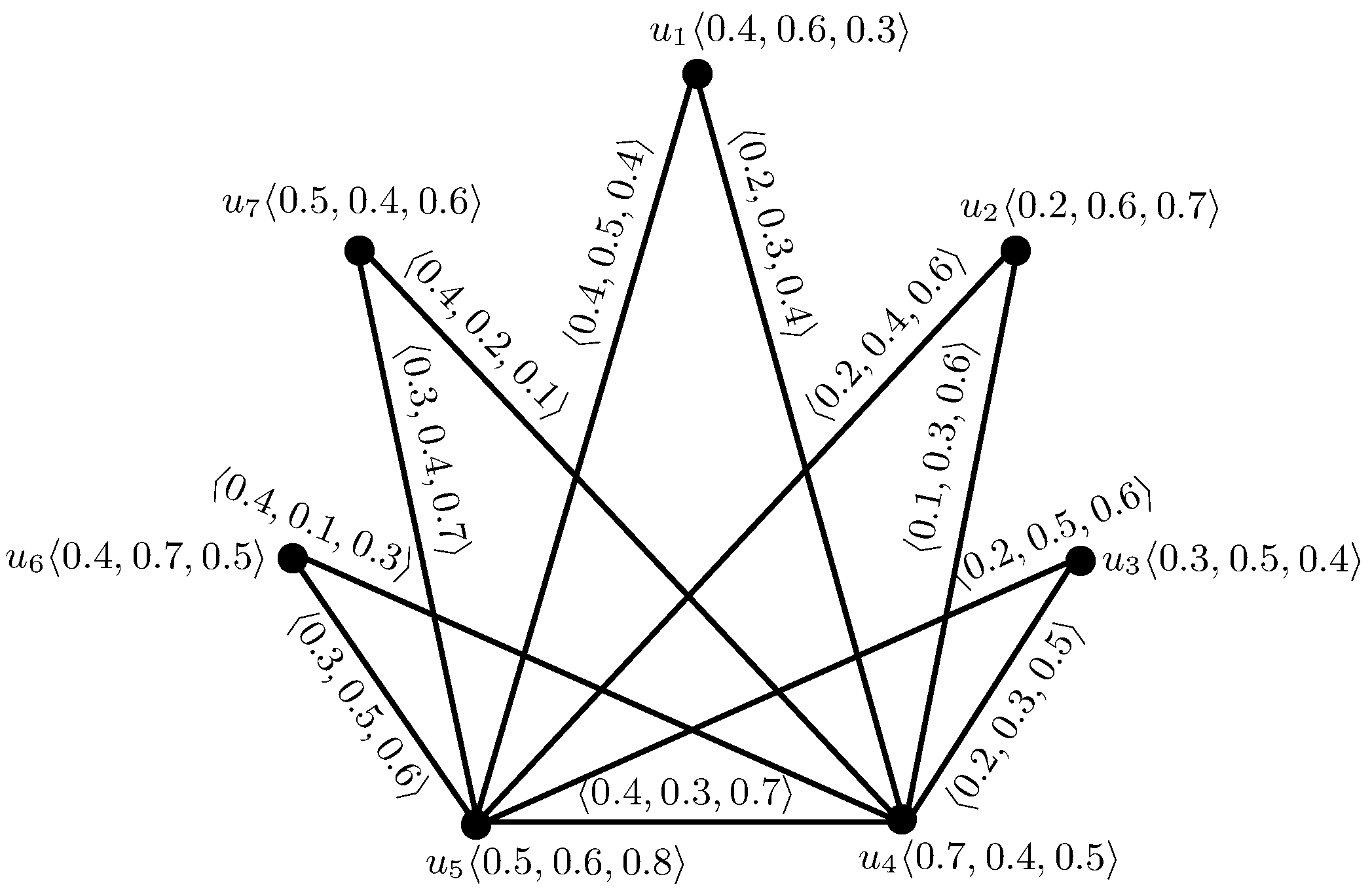
3. Laplacian Energy of Single-Valued Neutrosophic Graphs

In this section, we define and investigate the Laplacian energy of a graph under single-valued neutrosophic environment and investigate its properties.

Definition 7.

Let $\mathcal{G}=(X,Y)$ be a SVNG on n vertices. The degree matrix, $D(\mathcal{G})=\langle D(T_Y(u_j{u}_k)),D(I_Y(u_j{u}_k)),D(F_Y(u_j{u}_k))\rangle =\left[d_{jk}\right],$ of $\mathcal{G}$ is a $n\times n$ diagonal matrix defined as:

$$d_{jk}=\left\{\begin{array}{cc}{d}_{\mathcal{G}}(u_j)\hfill & \mathrm{if}j=k,\hfill \\ 0\hfill & \mathrm{otherwise}\hfill \end{array}\right.$$

Definition 8.

The Laplacian matrix of a SVNG $\mathcal{G}=(X,Y)$ is defined as $L(\mathcal{G})=\langle L(T_Y(u_j{u}_k)),L(I_Y(u_j{u}_k)),L(F_Y(u_j{u}_k))\rangle =D(\mathcal{G})-A(\mathcal{G})$, where $A(\mathcal{G})$ is an adjacency matrix and $D(\mathcal{G})$ is a degree matrix of a SVNG $\mathcal{G}$.

Definition 9.

The spectrum of Laplacian matrix of a SVNG $L(\mathcal{G})$ is defined as $\langle M_L,N_L,O_L\rangle$, where $M_L$, $N_L$ and $O_L$ are the sets of Laplacian eigenvalues of $L(T_Y(u_j{u}_k))$, $L(I_Y(u_j{u}_k))$ and $L(F_Y(u_j{u}_k))$, respectively.

Example 4.

Consider a SVNG $\mathcal{G}=(X,Y)$ of a graph $G=(V,E)$, where $V=\{u_1,u_2,u_3,u_4,u_5,u_6,u_7\}$ and $E=\{u_1{u}_4,u_1{u}_5,u_2{u}_4,u_2{u}_5,u_3{u}_4,u_3{u}_5,u_6{u}_4,u_6{u}_5,u_7{u}_4,u_7{u}_5\}$, as shown in Figure 2.

The adjacency and the Laplacian matrices of the SVNG shown in Figure 2 are as follows:

$$A(\mathcal{G})=\left(\begin{array}{ccccccc}\langle 0,0,0\rangle & \langle 0,0,0\rangle & \langle 0,0,0\rangle & \langle 0.2,0.3,0.4\rangle & \langle 0.4,0.5,0.4\rangle & \langle 0,0,0\rangle & \langle 0,0,0\rangle \\ \langle 0,0,0\rangle & \langle 0,0,0\rangle & \langle 0,0,0\rangle & \langle 0.1,0.3,0.6\rangle & \langle 0.2,0.4,0.6\rangle & \langle 0,0,0\rangle & \langle 0,0,0\rangle \\ \langle 0,0,0\rangle & \langle 0,0,0\rangle & \langle 0,0,0\rangle & \langle 0.2,0.3,0.5\rangle & \langle 0.2,0.5,0.6\rangle & \langle 0,0,0\rangle & \langle 0,0,0\rangle \\ \langle 0.2,0.3,0.4\rangle & \langle 0.1,0.3,0.6\rangle & \langle 0.2,0.3,0.5\rangle & \langle 0,0,0\rangle & \langle 0.4,0.3,0.7\rangle & \langle 0.4,0.1,0.3\rangle & \langle 0.4,0.2,0.1\rangle \\ \langle 0.4,0.5,0.4\rangle & \langle 0.2,0.4,0.6\rangle & \langle 0.2,0.5,0.6\rangle & \langle 0.4,0.3,0.7\rangle & \langle 0,0,0\rangle & \langle 0.3,0.5,0.6\rangle & \langle 0.3,0.4,0.7\rangle \\ \langle 0,0,0\rangle & \langle 0,0,0\rangle & \langle 0,0,0\rangle & \langle 0.4,0.1,0.3\rangle & \langle 0.3,0.5,0.6\rangle & \langle 0,0,0\rangle & \langle 0,0,0\rangle \\ \langle 0,0,0\rangle & \langle 0,0,0\rangle & \langle 0,0,0\rangle & \langle 0.4,0.2,0.1\rangle & \langle 0.3,0.4,0.7\rangle & \langle 0,0,0\rangle & \langle 0,0,0\rangle \end{array}\right).$$

$$L(\mathcal{G})=\left(\begin{array}{ccccccc}\langle 0.6,0.8,0.8\rangle & \langle 0,0,0\rangle & \langle 0,0,0\rangle & \langle -0.2,-0.3,-0.4\rangle & \langle -0.4,-0.5,-0.4\rangle & \langle 0,0,0\rangle & \langle 0,0,0\rangle \\ \langle 0,0,0\rangle & \langle 0.3,0.7,1.2\rangle & \langle 0,0,0\rangle & \langle -0.1,-0.3,-0.6\rangle & \langle -0.2,-0.4,-0.6\rangle & \langle 0,0,0\rangle & \langle 0,0,0\rangle \\ \langle 0,0,0\rangle & \langle 0,0,0\rangle & \langle 0.4,0.8,1.1\rangle & \langle -0.2,-0.3,-0.5\rangle & \langle -0.2,-0.5,-0.6\rangle & \langle 0,0,0\rangle & \langle 0,0,0\rangle \\ \langle -0.2,-0.3,-0.4\rangle & \langle -0.1,-0.3,-0.6\rangle & \langle -0.2,-0.3,-0.5\rangle & \langle 1.7,1.5,2.6\rangle & \langle -0.4,-0.3,-0.7\rangle & \langle -0.4,-0.1,-0.3\rangle & \langle -0.4,-0.2,-0.1\rangle \\ \langle -0.4,-0.5,-0.4\rangle & \langle -0.2,-0.4,-0.6\rangle & \langle -0.2,-0.5,-0.6\rangle & \langle -0.4,-0.3,-0.7\rangle & \langle 1.8,2.6,3.6\rangle & \langle -0.3,-0.5,-0.6\rangle & \langle -0.3,-0.4,-0.7\rangle \\ \langle 0,0,0\rangle & \langle 0,0,0\rangle & \langle 0,0,0\rangle & \langle -0.4,-0.1,-0.3\rangle & \langle -0.3,-0.5,-0.6\rangle & \langle 0.7,0.6,0.9\rangle & \langle 0,0,0\rangle \\ \langle 0,0,0\rangle & \langle 0,0,0\rangle & \langle 0,0,0\rangle & \langle -0.4,-0.2,-0.1\rangle & \langle -0.3,-0.4,-0.7\rangle & \langle 0,0,0\rangle & \langle 0.7,0.6,0.8\rangle \end{array}\right).$$

The Laplacian spectrum of a SVNG $\mathcal{G}$, given in Figure 2 is

$$\begin{array}{c}\text{Laplacian Spec}(T_Y(u_j{u}_k))=\{-0.8857,-0.5652,-0.4422,-0.2754,-0.1857,1.0605,1.2939\},\hfill \\ \text{Laplacian Spec}(I_Y(u_j{u}_k))=\{-1.0857,-0.4950,-0.4533,-0.3485,-0.2857,0.6952,1.9731\},\hfill \\ \text{Laplacian Spec}(F_Y(u_j{u}_k))=\{-1.5714,-0.8065,-0.7191,-0.5957,-0.4212,1.4560,2.6581\}.\hfill \end{array}$$

Therefore,

$$\begin{array}{ccc}\text{Laplacian Spec}(\mathcal{G})\hfill & =\hfill & \{\langle -0.8857,-1.0857,-1.5714\rangle ,\langle -0.5652,-0.4950,-0.8065\rangle ,\langle -0.4422,-0.4533,-0.7191\rangle ,\hfill \\ & & \langle -0.2754,-0.3485,-0.5957\rangle ,\langle -0.1857,-0.2857,-0.4212\rangle ,\langle 1.0605,0.6952,1.4560\rangle ,\hfill \\ & & \langle 1.2939,1.9731,2.6581\rangle \}.\hfill \end{array}$$

Theorem 3.

Let $\mathcal{G}=(X,Y)$ be a SVNG and let $L(\mathcal{G})=\langle L(T_Y(u_j{u}_k)),L(I_Y(u_j{u}_k)),L(F_Y(u_j{u}_k))\rangle$ be the Laplacian matrix of $\mathcal{G}$. If ${\vartheta }_1\ge {\vartheta }_2\ge \dots \ge {\vartheta }_n$, ${\phi }_1\ge {\phi }_2\ge \dots \ge {\phi }_n$ and ${\psi }_1\ge {\psi }_2\ge \dots \ge {\psi }_n$ are the eigenvalues of $L(T_Y(u_j{u}_k))$, $L(I_Y(u_j{u}_k))$ and $L(F_Y(u_j{u}_k))$, respectively. Then

• ${\displaystyle \sum _{\begin{array}{c}j=1\\ {\vartheta }_j\in M_L\end{array}}^n}{\vartheta }_j=2{\displaystyle \sum _{1\le j<k\le n}}{T}_Y(u_j{u}_k),{\displaystyle \sum _{\begin{array}{c}j=1\\ {\phi }_j\in N_L\end{array}}^n}{\phi }_j=2{\displaystyle \sum _{1\le j<k\le n}}{I}_Y(u_j{u}_k)$ and ${\displaystyle \sum _{\begin{array}{c}j=1\\ {\psi }_j\in O_L\end{array}}^n}{\psi }_j=2{\displaystyle \sum _{1\le j<k\le n}}{F}_Y(u_j{u}_k)$
• ${\displaystyle \sum _{\begin{array}{c}j=1\\ {\vartheta }_j\in M_L\end{array}}^n}{\vartheta }_j^2=2{\displaystyle \sum _{1\le j<k\le n}}{(T_Y(u_j{u}_k))}^2+{\displaystyle \sum _{j=1}^n}{d}_{T_Y(u_j{u}_k)}^2(u_j)$, ${\displaystyle \sum _{\begin{array}{c}j=1\\ {\phi }_j\in N_L\end{array}}^n}{\phi }_j^2=2{\displaystyle \sum _{1\le j<k\le n}}{(I_Y(u_j{u}_k))}^2+{\displaystyle \sum _{j=1}^n}{d}_{I_Y(u_j{u}_k)}^2(u_j)$ and ${\displaystyle \sum _{\begin{array}{c}j=1\\ {\psi }_j\in O_L\end{array}}^n}{\psi }_j^2=2{\displaystyle \sum _{1\le j<k\le n}}{(F_Y(u_j{u}_k))}^2+{\displaystyle \sum _{j=1}^n}{d}_{F_Y(u_j{u}_k)}^2(u_j)$.

Proof. 

• Since $L(\mathcal{G})$ is a symmetric matrix with non-negative Laplacian eigenvalues, such that

  $${\displaystyle \sum _{\begin{array}{c}j=1\\ {\vartheta }_j\in M_L\end{array}}^n}{\vartheta }_j=tr(L(\mathcal{G}))={\displaystyle \sum _{j=1}^n}{d}_{T_Y(u_j{u}_k)}(u_j)=2{\displaystyle \sum _{1\le j<k\le n}}{T}_Y(u_j{u}_k).$$
  Similarly, it is easy to show that, ${\displaystyle \sum _{\begin{array}{c}j=1\\ {\phi }_j\in N_L\end{array}}^n}{\phi }_j=2{\displaystyle \sum _{1\le j<k\le n}}{I}_Y(u_j{u}_k)$ and ${\displaystyle \sum _{\begin{array}{c}j=1\\ {\psi }_j\in O_L\end{array}}^n}{\psi }_j=2{\displaystyle \sum _{1\le j<k\le n}}{F}_Y(u_j{u}_k).$
• By definition of Laplacian matrix, we have

  $$L(T_Y(u_j{u}_k))=\left(\begin{array}{cccc}{d}_{T_Y(u_j{u}_k)}(u_1)& -T_Y(u_1{u}_2)& \dots & -T_Y(u_1{u}_n)\\ -T_Y(u_2{u}_1)& d_{T_Y(u_j{u}_k)}(u_2)& \dots & -T_Y(u_2{u}_n)\\ ⋮& ⋮& \ddots & ⋮\\ -T_Y(u_n{u}_1)& -T_Y(u_n{u}_2)& \dots & d_{T_Y(u_j{u}_k)}(u_n)\end{array}\right).$$

By trace properties of a matrix, we have

$$tr({(L(T_Y(u_j{u}_k)))}^2)={\displaystyle \sum _{\begin{array}{c}j=1\\ {\vartheta }_j\in M_L\end{array}}^n}{\vartheta }_j^2$$

where

$$\begin{array}{ccc}\hfill tr({(L(T_Y(u_j{u}_k)))}^2)& =& (d_{T_Y(u_j{u}_k)}^2(u_1)+T_Y^2(u_1{u}_2)+\dots +T_Y^2(u_1{u}_n))\hfill \\ & & +(T_Y^2(u_2{u}_1)+d_{T_Y(u_j{u}_k)}^2(u_2)+\dots +T_Y^2(u_2{u}_n))\hfill \\ & & +\dots +(T_Y^2(u_n{u}_1)+T_Y^2(u_n{u}_2)+\dots +d_{T_Y(u_j{u}_k)}^2(u_n))\hfill \\ & =& 2{\displaystyle \sum _{1\le j<k\le n}}{(T_Y(u_j{u}_k))}^2+{\displaystyle \sum _{j=1}^n}{d}_{T_Y(u_j{u}_k)}^2(u_j).\hfill \end{array}$$

Therefore,

$${\displaystyle \sum _{\begin{array}{c}j=1\\ {\vartheta }_j\in M_L\end{array}}^n}{\vartheta }_j^2=2\sum _{1\le j<k\le n}{(T_Y(u_j{u}_k))}^2+{\displaystyle \sum _{j=1}^n}{d}_{T_Y(u_j{u}_k)}^2(u_j).$$

Analogously, we can show that ${\displaystyle \sum _{\begin{array}{c}j=1\\ {\phi }_j\in N_L\end{array}}^n}{\phi }_j^2=2{\displaystyle \sum _{1\le j<k\le n}}{(I_Y(u_j{u}_k))}^2+{\displaystyle \sum _{j=1}^n}{d}_{I_Y(u_j{u}_k)}^2(u_j)$ and ${\displaystyle \sum _{\begin{array}{c}j=1\\ {\psi }_j\in O_L\end{array}}^n}{\psi }_j^2=2{\displaystyle \sum _{1\le j<k\le n}}{(F_Y(u_j{u}_k))}^2+{\displaystyle \sum _{j=1}^n}{d}_{F_Y(u_j{u}_k)}^2(u_j)$. ☐

Definition 10.

The Laplacian energy of a SVNG $\mathcal{G}=(X,Y)$ is defined as

$$LE(\mathcal{G})=〈LE(T_Y(u_j{u}_k)),LE(I_Y(u_j{u}_k)),LE(F_Y(u_j{u}_k))〉=〈\sum _{j=1}^n|{\varrho }_j|,\sum _{j=1}^n|{\xi }_j|,\sum _{j=1}^n|{\tau }_j|〉$$

where

$$\begin{array}{c}\hfill {\varrho }_j={\vartheta }_j-\frac{2{\displaystyle \sum _{1\le j<k\le n}}{T}_Y(u_j{u}_k)}{n},{\xi }_j={\phi }_j-\frac{2{\displaystyle \sum _{1\le j<k\le n}}{I}_Y(u_j{u}_k)}{n},{\tau }_j={\psi }_j-\frac{2{\displaystyle \sum _{1\le j<k\le n}}{F}_Y(u_j{u}_k)}{n}.\end{array}$$

Theorem 4.

Let $\mathcal{G}=(X,Y)$ be a SVNG and let $L(\mathcal{G})$ be the Laplacian matrix of $\mathcal{G}$. If ${\vartheta }_1\ge {\vartheta }_2\ge \dots \ge {\vartheta }_n$, ${\phi }_1\ge {\phi }_2\ge \dots \ge {\phi }_n$ and ${\psi }_1\ge {\psi }_2\ge \dots \ge {\psi }_n$ are the eigenvalues of $L(T_Y(u_j{u}_k))$, $L(I_Y(u_j{u}_k))$ and $L(F_Y(u_j{u}_k))$, respectively, and ${\varrho }_j={\vartheta }_j-\frac{2{\displaystyle \sum _{1\le j<k\le n}}{T}_Y(u_j{u}_k)}{n},{\xi }_j={\phi }_j-\frac{2{\displaystyle \sum _{1\le j<k\le n}}{I}_Y(u_j{u}_k)}{n},{\tau }_j={\psi }_j-\frac{2{\displaystyle \sum _{1\le j<k\le n}}{F}_Y(u_j{u}_k)}{n}.$ Then

$$\begin{array}{c}{\displaystyle \sum _{j=1}^n}{\varrho }_j=0,{\displaystyle \sum _{j=1}^n}{\xi }_j=0,{\displaystyle \sum _{j=1}^n}{\tau }_j=0,\hfill \\ {\displaystyle \sum _{j=1}^n}{\varrho }_j^2=2{\mathcal{M}}_T,{\displaystyle \sum _{j=1}^n}{\xi }_j^2=2{\mathcal{M}}_I,{\displaystyle \sum _{j=1}^n}{\tau }_j^2=2{\mathcal{M}}_F,\hfill \end{array}$$

where

$${\mathcal{M}}_T={\displaystyle \sum _{1\le j<k\le n}}{(T_Y(u_j{u}_k))}^2+\frac{1}{2}{\displaystyle \sum _{j=1}^n}{\left(d_{T_Y(u_j{u}_k)}(u_j)-\frac{2{\displaystyle \sum _{1\le j<k\le n}}{T}_Y(u_j{u}_k)}{n}\right)}^2,$$

$${\mathcal{M}}_I={\displaystyle \sum _{1\le j<k\le n}}{(I_Y(u_j{u}_k))}^2+\frac{1}{2}{\displaystyle \sum _{j=1}^n}{\left(d_{I_Y(u_j{u}_k)}(u_j)-\frac{2{\displaystyle \sum _{1\le j<k\le n}}{I}_Y(u_j{u}_k)}{n}\right)}^2,$$

$${\mathcal{M}}_F={\displaystyle \sum _{1\le j<k\le n}}{(F_Y(u_j{u}_k))}^2+\frac{1}{2}{\displaystyle \sum _{j=1}^n}{\left(d_{F_Y(u_j{u}_k)}(u_j)-\frac{2{\displaystyle \sum _{1\le j<k\le n}}{F}_Y(u_j{u}_k)}{n}\right)}^2.$$

Example 5.

Consider a SVNG $\mathcal{G}=(X,Y)$ on $V=\{u_1,u_2,u_3,u_4,u_5,u_6,u_7\}$, as shown in Figure 2. Then $LE(T_Y(u_j{u}_k))=4.7086,LE(I_Y(u_j{u}_k))=5.3364,LE(F_Y(u_j{u}_k))=8.2279.$

Therefore, $LE(\mathcal{G})=\langle 4.7086,5.3364,8.2279\rangle$. Also we have

$${\displaystyle \sum _{j=1}^7}{\varrho }_j=0,{\displaystyle \sum _{j=1}^7}{\xi }_j=0,{\displaystyle \sum _{j=1}^7}{\tau }_j=0.$$

$${\displaystyle \sum _{j=1}^7}{\varrho }_j^2=4.2086=2(2.1043)=2{\mathcal{M}}_T,$$

$${\displaystyle \sum _{j=1}^7}{\xi }_j^2=6.2086=2(3.1043)=2{\mathcal{M}}_I,$$

$${\displaystyle \sum _{j=1}^7}{\tau }_j^2=13.3543=2(6.6771)=2{\mathcal{M}}_F.$$

Theorem 5.

Let $\mathcal{G}=(X,Y)$ be a SVNG on n vertices and let $L(\mathcal{G})=\langle L(T_Y(u_j{u}_k)),L(I_Y(u_j{u}_k)),L(F_Y(u_j{u}_k))\rangle$ be the Laplacian matrix of $\mathcal{G}$. Then

(i) 

$LE(T_Y(u_j{u}_k))\le \sqrt{2n{\displaystyle \sum _{1\le j<k\le n}}{(T_Y(u_j{u}_k))}^2+n{\displaystyle \sum _{j=1}^n}{\left(d_{T_Y(u_j{u}_k)}(u_j)-\frac{2{\displaystyle \sum _{1\le j<k\le n}}{T}_Y(u_j{u}_k)}{n}\right)}^2};$

(ii) 

$LE(I_Y(u_j{u}_k))\le \sqrt{2n{\displaystyle \sum _{1\le j<k\le n}}{(I_Y(u_j{u}_k))}^2+n{\displaystyle \sum _{j=1}^n}{\left(d_{I_Y(u_j{u}_k)}(u_j)-\frac{2{\displaystyle \sum _{1\le j<k\le n}}{I}_Y(u_j{u}_k)}{n}\right)}^2};$

(iii) 

$LE(F_Y(u_j{u}_k))\le \sqrt{2n{\displaystyle \sum _{1\le j<k\le n}}{(F_Y(u_j{u}_k))}^2+n{\displaystyle \sum _{j=1}^n}{\left(d_{F_Y(u_j{u}_k)}(u_j)-\frac{2{\displaystyle \sum _{1\le j<k\le n}}{F}_Y(u_j{u}_k)}{n}\right)}^2}$.

Proof. 

Apply Cauchy-Schwarz inequality to the n numbers $1,1,\dots ,1$ and $|{\varrho }_1|,|{\varrho }_2|,\dots ,|{\varrho }_n|$, we have

$${\displaystyle \sum _{j=1}^n}|{\varrho }_j|\le \sqrt{n}\sqrt{{\displaystyle \sum _{j=1}^n}{|{\varrho }_j|}^2}$$

$$LE(T_Y(u_j{u}_k))\le \sqrt{n}\sqrt{2{\mathcal{M}}_T}=\sqrt{2n{\mathcal{M}}_T}.$$

Since ${\mathcal{M}}_T={\displaystyle \sum _{1\le j<k\le n}}{(T_Y(u_j{u}_k))}^2+\frac{1}{2}{\displaystyle \sum _{j=1}^n}{\left(d_{T_Y(u_j{u}_k)}(u_j)-\frac{2{\displaystyle \sum _{1\le j<k\le n}}{T}_Y(u_j{u}_k)}{n}\right)}^2,$ therefore, $LE(T_Y(u_j{u}_k))\le \sqrt{2n{\displaystyle \sum _{1\le j<k\le n}}{(T_Y(u_j{u}_k))}^2+n{\displaystyle \sum _{j=1}^n}{\left(d_{T_Y(u_j{u}_k)}(u_j)-\frac{2{\displaystyle \sum _{1\le j<k\le n}}{T}_Y(u_j{u}_k)}{n}\right)}^2}.$

Analogously, it is easy to show that $LE(I_Y(u_j{u}_k))\le \sqrt{2n{\displaystyle \sum _{1\le j<k\le n}}{(I_Y(u_j{u}_k))}^2+n{\displaystyle \sum _{j=1}^n}{\left(d_{I_Y(u_j{u}_k)}(u_j)-\frac{2{\displaystyle \sum _{1\le j<k\le n}}{I}_Y(u_j{u}_k)}{n}\right)}^2}$ and $LE(F_Y(u_j{u}_k))\le \sqrt{2n{\displaystyle \sum _{1\le j<k\le n}}{(F_Y(u_j{u}_k))}^2+n{\displaystyle \sum _{j=1}^n}{\left(d_{F_Y(u_j{u}_k)}(u_j)-\frac{2{\displaystyle \sum _{1\le j<k\le n}}{F}_Y(u_j{u}_k)}{n}\right)}^2}$. ☐

Theorem 6.

Let $\mathcal{G}=(X,Y)$ be a SVNG on n vertices and let $L(\mathcal{G})=\langle L(T_Y(u_j{u}_k)),L(I_Y(u_j{u}_k)),L(F_Y(u_j{u}_k))\rangle$ be the Laplacian matrix of $\mathcal{G}$. Then

(i) 

$LE(T_Y(u_j{u}_k))\ge 2\sqrt{{\displaystyle \sum _{1\le j<k\le n}}{(T_Y(u_j{u}_k))}^2+\frac{1}{2}{\displaystyle \sum _{j=1}^n}{\left(d_{T_Y(u_j{u}_k)}(u_j)-\frac{2{\displaystyle \sum _{1\le j<k\le n}}{T}_Y(u_j{u}_k)}{n}\right)}^2};$

(ii) 

$LE(I_Y(u_j{u}_k))\ge 2\sqrt{{\displaystyle \sum _{1\le j<k\le n}}{(I_Y(u_j{u}_k))}^2+\frac{1}{2}{\displaystyle \sum _{j=1}^n}{\left(d_{I_Y(u_j{u}_k)}(u_j)-\frac{2{\displaystyle \sum _{1\le j<k\le n}}{I}_Y(u_j{u}_k)}{n}\right)}^2};$

(iii) 

$LE(F_Y(u_j{u}_k))\ge 2\sqrt{{\displaystyle \sum _{1\le j<k\le n}}{(F_Y(u_j{u}_k))}^2+\frac{1}{2}{\displaystyle \sum _{j=1}^n}{\left(d_{F_Y(u_j{u}_k)}(u_j)-\frac{2{\displaystyle \sum _{1\le j<k\le n}}{F}_Y(u_j{u}_k)}{n}\right)}^2}$.

Proof. 

$${\left(\sum _{j=1}^n|{\varrho }_j|\right)}^2={\displaystyle \sum _{j=1}^n}|{\varrho }_j{|}^2+2\sum _{1\le j<k\le n}|{\varrho }_j{\varrho }_k|\ge 4{\mathcal{M}}_T$$

$$LE(T_Y(u_j{u}_k))\ge 2\sqrt{{\mathcal{M}}_T}$$

Since ${\mathcal{M}}_T={\displaystyle \sum _{1\le j<k\le n}}{(T_Y(u_j{u}_k))}^2+\frac{1}{2}{\displaystyle \sum _{j=1}^n}{\left(d_{T_Y(u_j{u}_k)}(u_j)-\frac{2{\displaystyle \sum _{1\le j<k\le n}}{T}_Y(u_j{u}_k)}{n}\right)}^2,$ therefore, $LE(T_Y(u_j{u}_k))\ge 2\sqrt{{\displaystyle \sum _{1\le j<k\le n}}{(T_Y(u_j{u}_k))}^2+\frac{1}{2}{\displaystyle \sum _{j=1}^n}{\left(d_{T_Y(u_j{u}_k)}(u_j)-\frac{2{\displaystyle \sum _{1\le j<k\le n}}{T}_Y(u_j{u}_k)}{n}\right)}^2}$.

Similarly, it is easy to show that $LE(I_Y(u_j{u}_k))\ge 2\sqrt{{\displaystyle \sum _{1\le j<k\le n}}{(I_Y(u_j{u}_k))}^2+\frac{1}{2}{\displaystyle \sum _{j=1}^n}{\left(d_{I_Y(u_j{u}_k)}(u_j)-\frac{2{\displaystyle \sum _{1\le j<k\le n}}{I}_Y(u_j{u}_k)}{n}\right)}^2}$ and $LE(F_Y(u_j{u}_k))\ge 2\sqrt{{\displaystyle \sum _{1\le j<k\le n}}{(F_Y(u_j{u}_k))}^2+\frac{1}{2}{\displaystyle \sum _{j=1}^n}{\left(d_{F_Y(u_j{u}_k)}(u_j)-\frac{2{\displaystyle \sum _{1\le j<k\le n}}{F}_Y(u_j{u}_k)}{n}\right)}^2}.$ ☐

Theorem 7.

Let $\mathcal{G}=(X,Y)$ be a SVNG on n vertices and let $L(\mathcal{G})=\langle L(T_Y(u_j{u}_k)),L(I_Y(u_j{u}_k)),L(F_Y(u_j{u}_k))\rangle$ be the Laplacian matrix of $\mathcal{G}$. Then

(i) 

$LE(T_Y(u_j{u}_k))\le |{\varrho }_1|+\sqrt{(n-1)\left(2{\displaystyle \sum _{1\le j<k\le n}}{(T_Y(u_j{u}_k))}^2+{\displaystyle \sum _{j=1}^n}{\left(d_{T_Y(u_j{u}_k)}(u_j)-\frac{2{\displaystyle \sum _{1\le j<k\le n}}{T}_Y(u_j{u}_k)}{n}\right)}^2-{\varrho }_1^2\right)};$

(ii) 

$LE(I_Y(u_j{u}_k))\le |{\xi }_1|+\sqrt{(n-1)\left(2{\displaystyle \sum _{1\le j<k\le n}}{(I_Y(u_j{u}_k))}^2+{\displaystyle \sum _{j=1}^n}{\left(d_{I_Y(u_j{u}_k)}(u_j)-\frac{2{\displaystyle \sum _{1\le j<k\le n}}{I}_Y(u_j{u}_k)}{n}\right)}^2-{\xi }_1^2\right)}$;

(iii) 

$LE(F_Y(u_j{u}_k))\le |{\tau }_1|+\sqrt{(n-1)\left(2{\displaystyle \sum _{1\le j<k\le n}}{(F_Y(u_j{u}_k))}^2+{\displaystyle \sum _{j=1}^n}{\left(d_{F_Y(u_j{u}_k)}(u_j)-\frac{2{\displaystyle \sum _{1\le j<k\le n}}{F}_Y(u_j{u}_k)}{n}\right)}^2-{\tau }_1^2\right)}.$

Proof. 

Using Cauchy-Schwarz inequality, we get

$${\displaystyle \sum _{j=1}^n}|{\varrho }_j|\le \sqrt{n{\displaystyle \sum _{j=1}^n}{|{\varrho }_j|}^2}$$

$${\displaystyle \sum _{j=2}^n}|{\varrho }_j|\le \sqrt{(n-1){\displaystyle \sum _{j=2}^n}{|{\varrho }_j|}^2}$$

$$LE(T_Y(u_j{u}_k))-|{\varrho }_1|\le \sqrt{(n-1)(2{\mathcal{M}}_T-{\varrho }_1^2)}$$

$$LE(T_Y(u_j{u}_k))\le |{\varrho }_1|+\sqrt{(n-1)(2{\mathcal{M}}_T-{\varrho }_1^2)}$$

Since ${\mathcal{M}}_T={\displaystyle \sum _{1\le j<k\le n}}{(T_Y(u_j{u}_k))}^2+\frac{1}{2}{\displaystyle \sum _{j=1}^n}{\left(d_{T_Y(u_j{u}_k)}(u_j)-\frac{2{\displaystyle \sum _{1\le j<k\le n}}{T}_Y(u_j{u}_k)}{n}\right)}^2,$ therefore

$$LE(T_Y(u_j{u}_k))\le |{\varrho }_1|+\sqrt{(n-1)\left(2{\displaystyle \sum _{1\le j<k\le n}}{(T_Y(u_j{u}_k))}^2+{\displaystyle \sum _{j=1}^n}{\left(d_{T_Y(u_j{u}_k)}(u_j)-\frac{2{\displaystyle \sum _{1\le j<k\le n}}{T}_Y(u_j{u}_k)}{n}\right)}^2-{\varrho }_1^2\right)}.$$

(3.1)

Similarly, we can show that $LE(I_Y(u_j{u}_k))\le |{\xi }_1|+\sqrt{(n-1)\left(2{\displaystyle \sum _{1\le j<k\le n}}{(I_Y(u_j{u}_k))}^2+{\displaystyle \sum _{j=1}^n}{\left(d_{I_Y(u_j{u}_k)}(u_j)-\frac{2{\displaystyle \sum _{1\le j<k\le n}}{I}_Y(u_j{u}_k)}{n}\right)}^2-{\xi }_1^2\right)}$ and $LE(F_Y(u_j{u}_k))\le |{\tau }_1|+\sqrt{(n-1)\left(2{\displaystyle \sum _{1\le j<k\le n}}{(F_Y(u_j{u}_k))}^2+{\displaystyle \sum _{j=1}^n}{\left(d_{F_Y(u_j{u}_k)}(u_j)-\frac{2{\displaystyle \sum _{1\le j<k\le n}}{F}_Y(u_j{u}_k)}{n}\right)}^2-{\tau }_1^2\right)}.$ ☐

Theorem 8.

If the SVNG $\mathcal{G}=(X,Y)$ is regular, then

(i) 

$LE(T_Y(u_j{u}_k))\le |{\varrho }_1|+\sqrt{(n-1)\left(2{\displaystyle \sum _{1\le j<k\le n}}{(T_Y(u_j{u}_k))}^2-{\varrho }_1^2\right)};$

(ii) 

$LE(I_Y(u_j{u}_k))\le |{\xi }_1|+\sqrt{(n-1)\left(2{\displaystyle \sum _{1\le j<k\le n}}{(I_Y(u_j{u}_k))}^2-{\xi }_1^2\right)};$

(iii) 

$LE(F_Y(u_j{u}_k))\le |{\tau }_1|+\sqrt{(n-1)\left(2{\displaystyle \sum _{1\le j<k\le n}}{(F_Y(u_j{u}_k))}^2-{\tau }_1^2\right)}.$

Proof. 

Let $\mathcal{G}$ be a regular SVNG, then

$$d_{T_Y(u_j{u}_k)}(u_j)=\frac{2{\displaystyle \sum _{1\le j<k\le n}}{T}_Y(u_j{u}_k)}{n}$$

(3.2)

Substituting (3.2) in (3.1), we get $LE(T_Y(u_j{u}_k))\le |{\varrho }_1|+\sqrt{(n-1)\left(2{\displaystyle \sum _{1\le j<k\le n}}{(T_Y(u_j{u}_k))}^2-{\varrho }_1^2\right)}$.

Similarly, it is easy to show that $LE(I_Y(u_j{u}_k))\le |{\xi }_1|+\sqrt{(n-1)\left(2{\displaystyle \sum _{1\le j<k\le n}}{(I_Y(u_j{u}_k))}^2-{\xi }_1^2\right)}$ and $LE(F_Y(u_j{u}_k))\le |{\tau }_1|+\sqrt{(n-1)\left(2{\displaystyle \sum _{1\le j<k\le n}}{(F_Y(u_j{u}_k))}^2-{\tau }_1^2\right)}.$ ☐

Theorem 9.

Let $\mathcal{G}=(X,Y)$ be a SVNG on n vertices with Laplacian matrix $L(\mathcal{G})=\langle L(T_Y(u_j{u}_k)),L(I_Y(u_j{u}_k)),L(F_Y(u_j{u}_k))\rangle$. Then

$$\begin{array}{c}LE(T_Y(u_j{u}_k))={\displaystyle \underset{1\le l\le n}{max}}\left\{2S_l(T_Y(u_j{u}_k))-\frac{4l{\displaystyle \sum _{1\le j<k\le n}}{T}_Y(u_j{u}_k)}{n}\right\},\hfill \\ LE(I_Y(u_j{u}_k))={\displaystyle \underset{1\le l\le n}{max}}\left\{2S_l(I_Y(u_j{u}_k))-\frac{4l{\displaystyle \sum _{1\le j<k\le n}}{I}_Y(u_j{u}_k)}{n}\right\},\hfill \\ LE(F_Y(u_j{u}_k))={\displaystyle \underset{1\le l\le n}{max}}\left\{2S_l(F_Y(u_j{u}_k))-\frac{4l{\displaystyle \sum _{1\le j<k\le n}}{F}_Y(u_j{u}_k)}{n}\right\},\hfill \end{array}$$

where $S_l(T_Y(u_j{u}_k))={\displaystyle \sum _{j=1}^l}{\vartheta }_j,$ $S_l(I_Y(u_j{u}_k))={\displaystyle \sum _{j=1}^l}{\phi }_j$ and $S_l(F_Y(u_j{u}_k))={\displaystyle \sum _{j=1}^l}{\psi }_j.$

4. Signless Laplacian Energy of Single-Valued Neutrosophic Graphs

Definition 11.

The signless Laplacian matrix of a SVNG $\mathcal{G}=(X,Y)$ is defined as $L^{+}(\mathcal{G})=\langle L^{+}(T_Y(u_j{u}_k)),L^{+}(I_Y(u_j{u}_k)),L^{+}(F_Y(u_j{u}_k))\rangle =D(\mathcal{G})+A(\mathcal{G})$, where $D(\mathcal{G})$ and $A(\mathcal{G})$ are the degree matrix and the adjacency matrix, respectively, of a SVNG $\mathcal{G}$.

Definition 12.

The spectrum of signless Laplacian matrix of a SVNG $L^{+}(\mathcal{G})$ is defined as $\langle M_{L^{+}},N_{L^{+}},O_{L^{+}}\rangle$, where $M_{L^{+}}$, $N_{L^{+}}$ and $O_{L^{+}}$ are the sets of signless Laplacian eigenvalues of $L^{+}(T_Y(u_j{u}_k))$, $L^{+}(I_Y(u_j{u}_k))$ and $L^{+}(F_Y(u_j{u}_k))$, respectively.

Example 6.

Consider a SVNG $\mathcal{G}=(X,Y)$ of a graph $G=(V,E)$, where $V=\{u_1,u_2,u_3,u_4,u_5,u_6,u_7\}$ and $E=\{u_1{u}_2,u_2{u}_3,u_3{u}_4,u_4{u}_5,u_5{u}_7,u_6{u}_7,u_6{u}_1,u_3{u}_5,u_1{u}_7,u_2{u}_7,u_3{u}_7\}$, as shown in Figure 3.

The adjacency and the signless Laplacian matrices of the SVNG, shown in Figure 3 are as follows:

$$A(\mathcal{G})=\left(\begin{array}{ccccccc}\langle 0,0,0\rangle & \langle 0.1,0.3,0.6\rangle & \langle 0,0,0\rangle & \langle 0,0,0\rangle & \langle 0,0,0\rangle & \langle 0.1,0.2,0.3\rangle & \langle 0.2,0.1,0.2\rangle \\ \langle 0.1,0.3,0.6\rangle & \langle 0,0,0\rangle & \langle 0.3,0.2,0.5\rangle & \langle 0,0,0\rangle & \langle 0,0,0\rangle & \langle 0,0,0\rangle & \langle 0.4,0.3,0.5\rangle \\ \langle 0,0,0\rangle & \langle 0.3,0.2,0.5\rangle & \langle 0,0,0\rangle & \langle 0.4,0.1,0.3\rangle & \langle 0.3,0.2,0.5\rangle & \langle 0,0,0\rangle & \langle 0.3,0.2,0.4\rangle \\ \langle 0,0,0\rangle & \langle 0,0,0\rangle & \langle 0.4,0.1,0.3\rangle & \langle 0,0,0\rangle & \langle 0.2,0.4,0.3\rangle & \langle 0,0,0\rangle & \langle 0,0,0\rangle \\ \langle 0,0,0\rangle & \langle 0,0,0\rangle & \langle 0.3,0.2,0.5\rangle & \langle 0.2,0.4,0.3\rangle & \langle 0,0,0\rangle & \langle 0,0,0\rangle & \langle 0.3,0.1,0.2\rangle \\ \langle 0.1,0.2,0.3\rangle & \langle 0,0,0\rangle & \langle 0,0,0\rangle & \langle 0,0,0\rangle & \langle 0,0,0\rangle & \langle 0,0,0\rangle & \langle 0.1,0.3,0.4\rangle \\ \langle 0.2,0.1,0.2\rangle & \langle 0.4,0.3,0.5\rangle & \langle 0.3,0.2,0.4\rangle & \langle 0,0,0\rangle & \langle 0.3,0.1,0.2\rangle & \langle 0.1,0.3,0.4\rangle & \langle 0,0,0\rangle \end{array}\right).$$

$$L^{+}(\mathcal{G})=\left(\begin{array}{ccccccc}\langle 0.4,0.6,1.1\rangle & \langle 0.1,0.3,0.6\rangle & \langle 0,0,0\rangle & \langle 0,0,0\rangle & \langle 0,0,0\rangle & \langle 0.1,0.2,0.3\rangle & \langle 0.2,0.1,0.2\rangle \\ \langle 0.1,0.3,0.6\rangle & \langle 0.8,0.8,1.6\rangle & \langle 0.3,0.2,0.5\rangle & \langle 0,0,0\rangle & \langle 0,0,0\rangle & \langle 0,0,0\rangle & \langle 0.4,0.3,0.5\rangle \\ \langle 0,0,0\rangle & \langle 0.3,0.2,0.5\rangle & \langle 1.3,0.7,1.7\rangle & \langle 0.4,0.1,0.3\rangle & \langle 0.3,0.2,0.5\rangle & \langle 0,0,0\rangle & \langle 0.3,0.2,0.4\rangle \\ \langle 0,0,0\rangle & \langle 0,0,0\rangle & \langle 0.4,0.1,0.3\rangle & \langle 0.6,0.5,0.6\rangle & \langle 0.2,0.4,0.3\rangle & \langle 0,0,0\rangle & \langle 0,0,0\rangle \\ \langle 0,0,0\rangle & \langle 0,0,0\rangle & \langle 0.3,0.2,0.5\rangle & \langle 0.2,0.4,0.3\rangle & \langle 0.8,0.7,1.0\rangle & \langle 0,0,0\rangle & \langle 0.3,0.1,0.2\rangle \\ \langle 0.1,0.2,0.3\rangle & \langle 0,0,0\rangle & \langle 0,0,0\rangle & \langle 0,0,0\rangle & \langle 0,0,0\rangle & \langle 0.2,0.5,0.7\rangle & \langle 0.1,0.3,0.4\rangle \\ \langle 0.2,0.1,0.2\rangle & \langle 0.4,0.3,0.5\rangle & \langle 0.3,0.2,0.4\rangle & \langle 0,0,0\rangle & \langle 0.3,0.1,0.2\rangle & \langle 0.1,0.3,0.4\rangle & \langle 1.3,1.0,1.7\rangle \end{array}\right).$$

The signless Laplacian spectrum of a SVNG $\mathcal{G}$, given in Figure 3 is

$$\begin{array}{c}\text{Signless Laplacian Spec}(T_Y(u_j{u}_k))=\{-0.6176,-0.4406,-0.3647,-0.3184,0.0300,0.4324,1.2792\},\hfill \\ \text{Signless Laplacian Spec}(I_Y(u_j{u}_k))=\{-0.5270,-0.4824,-0.2533,-0.0297,0.0686,0.3889,0.8349\},\hfill \\ \text{Signless Laplacian Spec}(F_Y(u_j{u}_k)=\{-0.8718,-0.7690,-0.5311,-0.2577,0.1719,0.5803,1.6774\}.\hfill \end{array}$$

Therefore,

$$\begin{array}{ccc}\text{Signless Laplacian Spec}(\mathcal{G})\hfill & =\hfill & \{\langle -0.6176,-0.5270,-0.8718\rangle ,\langle -0.4406,-0.4824,-0.7690\rangle ,\langle -0.3647,\hfill \\ & & -0.2533,-0.5311\rangle ,\langle -0.3184,-0.0297,-0.2577\rangle ,\langle 0.0300,0.0686,0.1719\rangle ,\hfill \\ & & \langle 0.4324,0.3889,0.5803\rangle ,\langle 1.2792,0.8349,1.6774\rangle \}.\hfill \end{array}$$

Theorem 10.

Let $\mathcal{G}=(X,Y)$ be a SVNG and let $L^{+}(\mathcal{G})$ be the signless Laplacian matrix of $\mathcal{G}$. If ${\vartheta }_1^{+}\ge {\vartheta }_2^{+}\ge \dots \ge {\vartheta }_n^{+}$, ${\phi }_1^{+}\ge {\phi }_2^{+}\ge \dots \ge {\phi }_n^{+}$ and ${\psi }_1^{+}\ge {\psi }_2^{+}\ge \dots \ge {\psi }_n^{+}$ are the eigenvalues of $L^{+}(T_Y(u_j{u}_k))$, $L^{+}(I_Y(u_j{u}_k))$ and $L^{+}(F_Y(u_j{u}_k))$, respectively. Then

1. 

${\displaystyle \sum _{\begin{array}{c}j=1\\ {\vartheta }_j^{+}\in M_{L^{+}}\end{array}}^n}{\vartheta }_j^{+}=2{\displaystyle \sum _{1\le j<k\le n}}{T}_Y(u_j{u}_k),{\displaystyle \sum _{\begin{array}{c}j=1\\ {\phi }_j^{+}\in N_{L^{+}}\end{array}}^n}{\phi }_j^{+}=2{\displaystyle \sum _{1\le j<k\le n}}{I}_Y(u_j{u}_k)$ and ${\displaystyle \sum _{\begin{array}{c}j=1\\ {\psi }_j^{+}\in O_{L^{+}}\end{array}}^n}{\psi }_j^{+}=2{\displaystyle \sum _{1\le j<k\le n}}{F}_Y(u_j{u}_k)$

2. 

${\displaystyle \sum _{\begin{array}{c}j=1\\ {\vartheta }_j^{+}\in M_{L^{+}}\end{array}}^n}{({\vartheta }_j^{+})}^2=2{\displaystyle \sum _{1\le j<k\le n}}{(T_Y(u_j{u}_k))}^2+{\displaystyle \sum _{j=1}^n}{d}_{T_Y(u_j{u}_k)}^2(u_j)$, ${\displaystyle \sum _{\begin{array}{c}j=1\\ {\phi }_j^{+}\in N_{L^{+}}\end{array}}^n}{({\phi }_j^{+})}^2=2{\displaystyle \sum _{1\le j<k\le n}}{(I_Y(u_j{u}_k))}^2+{\displaystyle \sum _{j=1}^n}{d}_{I_Y(u_j{u}_k)}^2(u_j)$ and ${\displaystyle \sum _{\begin{array}{c}j=1\\ {\psi }_j^{+}\in O_{L^{+}}\end{array}}^n}{({\psi }_j^{+})}^2=2{\displaystyle \sum _{1\le j<k\le n}}{(F_Y(u_j{u}_k))}^2+{\displaystyle \sum _{j=1}^n}{d}_{F_Y(u_j{u}_k)}^2(u_j)$.

Proof. 

Proof follows at once from proof of Theorem 3. ☐

Definition 13.

The signless Laplacian energy of a SVNG $\mathcal{G}=(X,Y)$ is defined as

$$L{E}^{+}(\mathcal{G})=〈L{E}^{+}(T_Y(u_j{u}_k)),L{E}^{+}(I_Y(u_j{u}_k)),L{E}^{+}(F_Y(u_j{u}_k))〉=〈\sum _{j=1}^n|{\varrho }_j^{+}|,\sum _{j=1}^n|{\xi }_j^{+}|,\sum _{j=1}^n|{\tau }_j^{+}|〉$$

where

$$\begin{array}{c}\hfill {\varrho }_j^{+}={\vartheta }_j^{+}-\frac{2{\displaystyle \sum _{1\le j<k\le n}}{T}_Y(u_j{u}_k)}{n},{\xi }_j^{+}={\phi }_j^{+}-\frac{2{\displaystyle \sum _{1\le j<k\le n}}{I}_Y(u_j{u}_k)}{n},{\tau }_j^{+}={\psi }_j^{+}-\frac{2{\displaystyle \sum _{1\le j<k\le n}}{F}_Y(u_j{u}_k)}{n}.\end{array}$$

Theorem 11.

Let $\mathcal{G}=(X,Y)$ be a SVNG and let $L^{+}(\mathcal{G})$ be the signless Laplacian matrix of $\mathcal{G}$. If ${\vartheta }_1^{+}\ge {\vartheta }_2^{+}\ge \dots \ge {\vartheta }_n^{+}$, ${\phi }_1^{+}\ge {\phi }_2^{+}\ge \dots \ge {\phi }_n^{+}$ and ${\psi }_1^{+}\ge {\psi }_2^{+}\ge \dots \ge {\psi }_n^{+}$ are the eigenvalues of $L^{+}(T_Y(u_j{u}_k))$, $L^{+}(I_Y(u_j{u}_k))$ and $L^{+}(F_Y(u_j{u}_k))$, respectively, and ${\varrho }_j^{+}={\vartheta }_j^{+}-\frac{2{\displaystyle \sum _{1\le j<k\le n}}{T}_Y(u_j{u}_k)}{n},{\xi }_j^{+}={\phi }_j^{+}-\frac{2{\displaystyle \sum _{1\le j<k\le n}}{I}_Y(u_j{u}_k)}{n},{\tau }_j^{+}={\psi }_j^{+}-\frac{2{\displaystyle \sum _{1\le j<k\le n}}{F}_Y(u_j{u}_k)}{n}.$ Then

$$\begin{array}{c}{\displaystyle \sum _{j=1}^n}{\varrho }_j^{+}=0,{\displaystyle \sum _{j=1}^n}{\xi }_j^{+}=0,{\displaystyle \sum _{j=1}^n}{\tau }_j^{+}=0,\hfill \\ {\displaystyle \sum _{j=1}^n}{({\varrho }_j^{+})}^2=2{\mathcal{M}}_T^{+},{\displaystyle \sum _{j=1}^n}{({\xi }_j^{+})}^2=2{\mathcal{M}}_I^{+},{\displaystyle \sum _{j=1}^n}{({\tau }_j^{+})}^2=2{\mathcal{M}}_F^{+},\hfill \end{array}$$

where

$$\begin{array}{c}{\mathcal{M}}_T^{+}={\displaystyle \sum _{1\le j<k\le n}}{(T_Y(u_j{u}_k))}^2+\frac{1}{2}{\displaystyle \sum _{j=1}^n}{\left(d_{T_Y(u_j{u}_k)}(u_j)-\frac{2{\displaystyle \sum _{1\le j<k\le n}}{T}_Y(u_j{u}_k)}{n}\right)}^2,\hfill \\ {\mathcal{M}}_I^{+}={\displaystyle \sum _{1\le j<k\le n}}{(I_Y(u_j{u}_k))}^2+\frac{1}{2}{\displaystyle \sum _{j=1}^n}{\left(d_{I_Y(u_j{u}_k)}(u_j)-\frac{2{\displaystyle \sum _{1\le j<k\le n}}{I}_Y(u_j{u}_k)}{n}\right)}^2,\hfill \\ {\mathcal{M}}_F^{+}={\displaystyle \sum _{1\le j<k\le n}}{(F_Y(u_j{u}_k))}^2+\frac{1}{2}{\displaystyle \sum _{j=1}^n}{\left(d_{F_Y(u_j{u}_k)}(u_j)-\frac{2{\displaystyle \sum _{1\le j<k\le n}}{F}_Y(u_j{u}_k)}{n}\right)}^2.\hfill \end{array}$$

Example 7.

Consider a SVNG $\mathcal{G}=(X,Y)$ on $V=\{u_1,u_2,u_3,u_4,u_5,u_6,u_7\}$, as shown in Figure 3. Then $L{E}^{+}(T_Y(u_j{u}_k))=3.4830,L{E}^{+}(I_Y(u_j{u}_k))=2.5848,L{E}^{+}(F_Y(u_j{u}_k))=4.8593.$

Therefore, $L{E}^{+}(\mathcal{G})=\langle 3.4830,2.5848,4.8593\rangle$. Also we have

$${\displaystyle \sum _{j=1}^7}{\varrho }_j^{+}=0,{\displaystyle \sum _{j=1}^7}{\xi }_j^{+}=0,{\displaystyle \sum _{j=1}^7}{\tau }_j^{+}=0.$$

$$\begin{array}{c}{\displaystyle \sum _{j=1}^7}{({\varrho }_j^{+})}^2=2.6343=2(1.3171)=2{\mathcal{M}}_T^{+},{\displaystyle \sum _{j=1}^7}{({\xi }_j^{+})}^2=1.4286=2(0.7143)=2{\mathcal{M}}_I^{+},\hfill \\ {\displaystyle \sum _{j=1}^7}{({\tau }_j^{+})}^2=4.8800=2(2.4400)=2{\mathcal{M}}_F^{+}.\hfill \end{array}$$

Theorem 12.

Let $\mathcal{G}=(X,Y)$ be a SVNG on n vertices with signless Laplacian matrix $L^{+}(\mathcal{G})=\langle L^{+}(T_Y(u_j{u}_k)),L^{+}(I_Y(u_j{u}_k)),L^{+}(F_Y(u_j{u}_k))\rangle$. Then

$$L{E}^{+}(T_Y(u_j{u}_k))=\underset{1\le l\le n}{max}\left\{2S_l^{+}(T_Y(u_j{u}_k))-\frac{4l{\displaystyle \sum _{1\le j<k\le n}}{T}_Y(u_j{u}_k)}{n}\right\},$$

$$L{E}^{+}(I_Y(u_j{u}_k))=\underset{1\le l\le n}{max}\left\{2S_l^{+}(I_Y(u_j{u}_k))-\frac{4l{\displaystyle \sum _{1\le j<k\le n}}{I}_Y(u_j{u}_k)}{n}\right\},$$

$$L{E}^{+}(F_Y(u_j{u}_k))=\underset{1\le l\le n}{max}\left\{2S_l^{+}(F_Y(u_j{u}_k))-\frac{4l{\displaystyle \sum _{1\le j<k\le n}}{F}_Y(u_j{u}_k)}{n}\right\},$$

where $S_l^{+}(T_Y(u_j{u}_k))={\displaystyle \sum _{j=1}^l}{\vartheta }_j^{+},$ $S_l^{+}(I_Y(u_j{u}_k))={\displaystyle \sum _{j=1}^l}{\phi }_j^{+}$ and $S_l^{+}(F_Y(u_j{u}_k))={\displaystyle \sum _{j=1}^l}{\psi }_j^{+}.$

5. Relation among Energy, Laplacian Energy and Signless Laplacian Energy of SVNGs

This section discusses the relationship among energy, Laplacian energy and signless Laplacian energy of SVNGs.

Theorem 13.

Let $\mathcal{G}$ be a SVNG on n vertices and let $A(\mathcal{G})$, $L(\mathcal{G})$ and $L^{+}(\mathcal{G})$ be the adjacency, the Laplacian and the signless Laplacian matrices of $\mathcal{G}$, respectively. Then $\left|L{E}^{+}(\mathcal{G})-LE(\mathcal{G})\right|\le 2E(\mathcal{G})$.

Proof. 

Clearly,

$$L^{+}(T_Y(u_j{u}_k))-\frac{2{\displaystyle \sum _{1\le j<k\le n}}{T}_Y(u_j{u}_k)}{n}=D(T_Y(u_j{u}_k))+A(T_Y(u_j{u}_k))-\frac{2{\displaystyle \sum _{1\le j<k\le n}}{T}_Y(u_j{u}_k)}{n}$$

(5.1)

$$L(T_Y(u_j{u}_k))-\frac{2{\displaystyle \sum _{1\le j<k\le n}}{T}_Y(u_j{u}_k)}{n}=D(T_Y(u_j{u}_k))-A(T_Y(u_j{u}_k))-\frac{2{\displaystyle \sum _{1\le j<k\le n}}{T}_Y(u_j{u}_k)}{n}$$

(5.2)

From Equations (5.1) and (5.2), we get

$$\left(L^{+}(T_Y(u_j{u}_k))-\frac{2{\displaystyle \sum _{1\le j<k\le n}}{T}_Y(u_j{u}_k)}{n}\right)-\left(L(T_Y(u_j{u}_k))-\frac{2{\displaystyle \sum _{1\le j<k\le n}}{T}_Y(u_j{u}_k)}{n}\right)=2A(T_Y(u_j{u}_k))$$

Then,

$$\left(L(T_Y(u_j{u}_k))-\frac{2{\displaystyle \sum _{1\le j<k\le n}}{T}_Y(u_j{u}_k)}{n}\right)=\left(L^{+}(T_Y(u_j{u}_k))-\frac{2{\displaystyle \sum _{1\le j<k\le n}}{T}_Y(u_j{u}_k)}{n}\right)-2A(T_Y(u_j{u}_k))$$

Also

$$\left(L^{+}(T_Y(u_j{u}_k))-\frac{2{\displaystyle \sum _{1\le j<k\le n}}{T}_Y(u_j{u}_k)}{n}\right)=2A(T_Y(u_j{u}_k))+\left(L(T_Y(u_j{u}_k))-\frac{2{\displaystyle \sum _{1\le j<k\le n}}{T}_Y(u_j{u}_k)}{n}\right)$$

By well known property of energy of a graph,

$$\begin{array}{ccc}LE(T_Y(u_j{u}_k))\hfill & =\hfill & E\left(L(T_Y(u_j{u}_k))-\frac{2{\displaystyle \sum _{1\le j<k\le n}}{T}_Y(u_j{u}_k)}{n}\right)\le E\left(L^{+}(T_Y(u_j{u}_k))-\frac{2{\displaystyle \sum _{1\le j<k\le n}}{T}_Y(u_j{u}_k)}{n}\right)\hfill \\ & & +E(-2A(T_Y(u_j{u}_k)))\hfill \\ & =\hfill & L{E}^{+}(T_Y(u_j{u}_k))+2E(T_Y(u_j{u}_k))\hfill \end{array}$$

(5.3)

$$\begin{array}{ccc}L{E}^{+}(T_Y(u_j{u}_k))\hfill & =\hfill & E\left(L^{+}(T_Y(u_j{u}_k))-\frac{2{\displaystyle \sum _{1\le j<k\le n}}{T}_Y(u_j{u}_k)}{n}\right)\le E\left(L(T_Y(u_j{u}_k))-\frac{2{\displaystyle \sum _{1\le j<k\le n}}{T}_Y(u_j{u}_k)}{n}\right)\hfill \\ & & +E(2A(T_Y(u_j{u}_k)))\hfill \\ & =\hfill & LE(T_Y(u_j{u}_k))+2E(T_Y(u_j{u}_k))\hfill \end{array}$$

(5.4)

Combining (5.3) and (5.4), we get $\left|L{E}^{+}(T_Y(u_j{u}_k))-LE(T_Y(u_j{u}_k))\right|\le 2E(T_Y(u_j{u}_k))$. Analogously, we can show that $\left|L{E}^{+}(I_Y(u_j{u}_k))-LE(I_Y(u_j{u}_k))\right|\le 2E(I_Y(u_j{u}_k))$ and $\left|L{E}^{+}(F_Y(u_j{u}_k))-LE(F_Y(u_j{u}_k))\right|\le 2E(F_Y(u_j{u}_k)).$ Hence $\left|L{E}^{+}(\mathcal{G})-LE(\mathcal{G})\right|\le 2E(\mathcal{G})$. ☐

Theorem 14.

If the SVNG $\mathcal{G}$ is regular. Then $E(\mathcal{G})=LE(\mathcal{G})=L{E}^{+}(\mathcal{G})$.

Theorem 15.

Let $\mathcal{G}=(X,Y)$ be a SVNG on n vertices and let $L(\mathcal{G})$ and $L^{+}(\mathcal{G})$ be the Laplacian and the signless Laplacian matrices of $\mathcal{G}$, respectively. Then

$$\begin{array}{c}L{E}^{+}(T_Y(u_j{u}_k))+LE(T_Y(u_j{u}_k))\ge max\left\{2E(T_Y(u_j{u}_k)),2{\displaystyle \sum _{j=1}^n}\left|d_{T_Y(u_j{u}_k)}(u_j)-\frac{2{\displaystyle \sum _{1\le j<k\le n}}{T}_Y(u_j{u}_k)}{n}\right|\right\},\hfill \\ L{E}^{+}(I_Y(u_j{u}_k))+LE(I_Y(u_j{u}_k))\ge max\left\{2E(I_Y(u_j{u}_k)),2{\displaystyle \sum _{j=1}^n}\left|d_{I_Y(u_j{u}_k)}(u_j)-\frac{2{\displaystyle \sum _{1\le j<k\le n}}{I}_Y(u_j{u}_k)}{n}\right|\right\},\hfill \\ L{E}^{+}(F_Y(u_j{u}_k))+LE(F_Y(u_j{u}_k))\ge max\left\{2E(F_Y(u_j{u}_k)),2{\displaystyle \sum _{j=1}^n}\left|d_{F_Y(u_j{u}_k)}(u_j)-\frac{2{\displaystyle \sum _{1\le j<k\le n}}{F}_Y(u_j{u}_k)}{n}\right|\right\}.\hfill \end{array}$$

Theorem 16.

Let $\mathcal{G}=(X,Y)$ be a SVNG on n vertices and let $L(\mathcal{G})$ and $L^{+}(\mathcal{G})$ be the Laplacian and the signless Laplacian matrices of $\mathcal{G}$, respectively. Then

$$L{E}^{+}(T_Y(u_j{u}_k))+LE(T_Y(u_j{u}_k))\ge 4E(T_Y(u_j{u}_k))-\frac{4r{\displaystyle \sum _{1\le j<k\le n}}{T}_Y(u_j{u}_k)}{n},$$

$$L{E}^{+}(I_Y(u_j{u}_k))+LE(I_Y(u_j{u}_k))\ge 4E(I_Y(u_j{u}_k))-\frac{4r{\displaystyle \sum _{1\le j<k\le n}}{I}_Y(u_j{u}_k)}{n},$$

$$L{E}^{+}(F_Y(u_j{u}_k))+LE(F_Y(u_j{u}_k))\ge 4E(F_Y(u_j{u}_k))-\frac{4r{\displaystyle \sum _{1\le j<k\le n}}{F}_Y(u_j{u}_k)}{n}$$

where r is the number of non-zero eigenvalues of SVNG $\mathcal{G}$.

Theorem 17.

Let $\mathcal{G}=(X,Y)$ be a SVNG on n vertices and let $L(\mathcal{G})=\langle L(T_Y(u_j{u}_k)),L(I_Y(u_j{u}_k)),L(F_Y(u_j{u}_k))\rangle$ be the Laplacian matrix of $\mathcal{G}$. Then

$$LE(T_Y(u_j{u}_k))\le E(T_Y(u_j{u}_k))+\sum _{j=1}^n\left|d_{T_Y(u_j{u}_k)}(u_j)-\frac{2{\displaystyle \sum _{1\le j<k\le n}}{T}_Y(u_j{u}_k)}{n}\right|,$$

$$LE(I_Y(u_j{u}_k))\le E(I_Y(u_j{u}_k))+\sum _{j=1}^n\left|d_{I_Y(u_j{u}_k)}(u_j)-\frac{2{\displaystyle \sum _{1\le j<k\le n}}{I}_Y(u_j{u}_k)}{n}\right|,$$

$$LE(F_Y(u_j{u}_k))\le E(F_Y(u_j{u}_k))+\sum _{j=1}^n\left|d_{F_Y(u_j{u}_k)}(u_j)-\frac{2{\displaystyle \sum _{1\le j<k\le n}}{F}_Y(u_j{u}_k)}{n}\right|.$$

Theorem 18.

Let $\mathcal{G}=(X,Y)$ be a SVNG on n vertices and let $L^{+}(\mathcal{G})=\langle L^{+}(T_Y(u_j{u}_k)),L^{+}(I_Y(u_j{u}_k)),L^{+}(F_Y(u_j{u}_k))\rangle$ be the signless Laplacian matrix of $\mathcal{G}$. Then

$$L{E}^{+}(T_Y(u_j{u}_k))\le E(T_Y(u_j{u}_k))+\sum _{j=1}^n\left|d_{T_Y(u_j{u}_k)}(u_j)-\frac{2{\displaystyle \sum _{1\le j<k\le n}}{T}_Y(u_j{u}_k)}{n}\right|,$$

$$L{E}^{+}(I_Y(u_j{u}_k))\le E(I_Y(u_j{u}_k))+\sum _{j=1}^n\left|d_{I_Y(u_j{u}_k)}(u_j)-\frac{2{\displaystyle \sum _{1\le j<k\le n}}{I}_Y(u_j{u}_k)}{n}\right|,$$

$$L{E}^{+}(F_Y(u_j{u}_k))\le E(F_Y(u_j{u}_k))+\sum _{j=1}^n\left|d_{F_Y(u_j{u}_k)}(u_j)-\frac{2{\displaystyle \sum _{1\le j<k\le n}}{F}_Y(u_j{u}_k)}{n}\right|.$$

Theorem 19.

Let $\mathcal{G}$ be a connected SVNG on n vertices and let $L^{+}(\mathcal{G})=\langle L^{+}(T_Y(u_j{u}_k)),L^{+}(I_Y(u_j{u}_k)),L^{+}(F_Y(u_j{u}_k))\rangle$ be the signless Laplacian matrix of $\mathcal{G}$. Then

$$L{E}^{+}(T_Y(u_j{u}_k))\le E(T_Y(u_j{u}_k))+\sqrt{n{\displaystyle \sum _{j=1}^n}{d}_{T_Y(u_j{u}_k)}^2(u_j)-4{\left(\sum _{1\le j<k\le n}{T}_Y(u_j{u}_k)\right)}^2},$$

$$L{E}^{+}(I_Y(u_j{u}_k))\le E(I_Y(u_j{u}_k))+\sqrt{n{\displaystyle \sum _{j=1}^n}{d}_{I_Y(u_j{u}_k)}^2(u_j)-4{\left(\sum _{1\le j<k\le n}{I}_Y(u_j{u}_k)\right)}^2},$$

$$L{E}^{+}(F_Y(u_j{u}_k))\le E(F_Y(u_j{u}_k))+\sqrt{n{\displaystyle \sum _{j=1}^n}{d}_{F_Y(u_j{u}_k)}^2(u_j)-4{\left(\sum _{1\le j<k\le n}{F}_Y(u_j{u}_k)\right)}^2}.$$

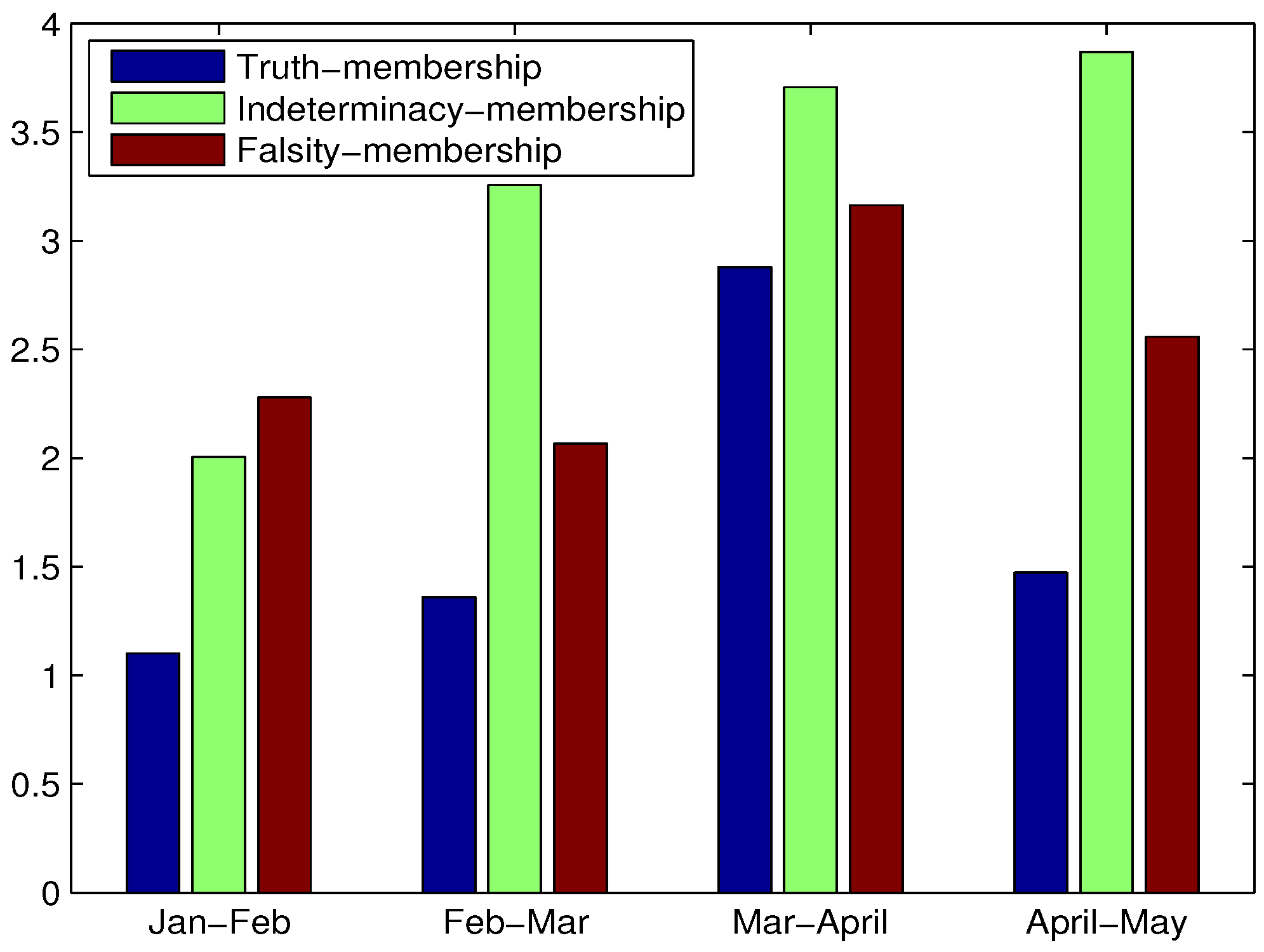
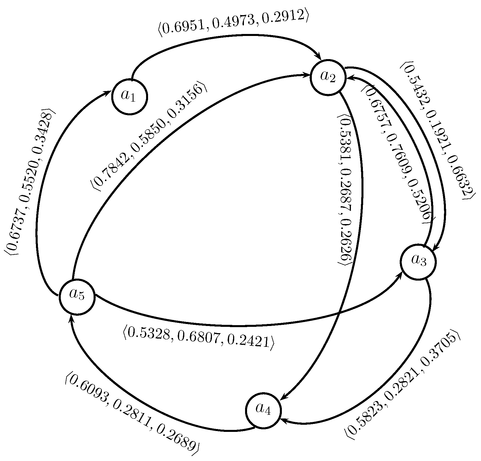
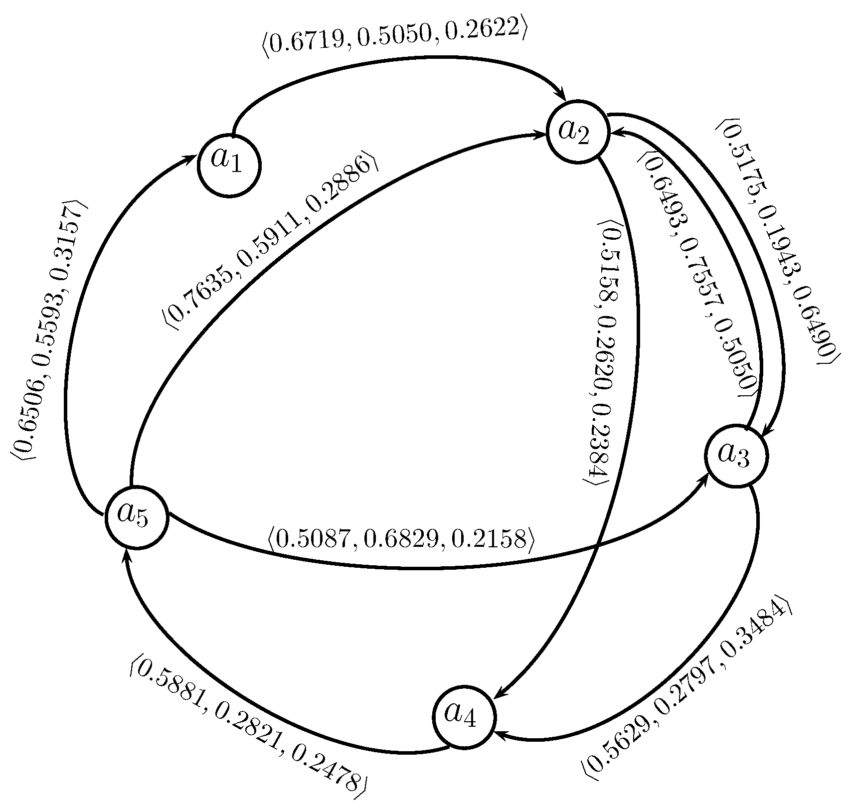
6. Application of Energy of SVNGs in Group Decision-Making

Group decision-making is a commonly used tool in human activities, which determines the optimal alternative from a given finite set of alternatives using the evaluation information given by a group of decision makers or experts. With the rapid development of society, group decision-making plays an increasingly important role when dealing with the decision-making problems. Recently, many scholars have investigated the approaches for group decision-making based on different kinds of decision information. However, in order to reflect the relationships among the alternatives, we need to make pairwise comparisons for all the alternatives in the process of decision- making. Preference relation is a powerful quantitative decision technique that support experts in expressing their preferences over the given alternatives. For a set of alternatives $Z=\{z_1,z_2,\dots ,z_n\}$, the experts compare each pair of alternatives and construct preference relations, respectively. If every element in the preference relations is a single-valued neutrosophic number, then the concept of the single-valued neutrosophic preference relation (SVNPR) can be put forth as follows:

Definition 14.

A SVNPR on the set $Z=\left\{z_1,z_2,\dots ,z_n\right\}$ is represented by a matrix $R={(r_{jk})}_{n\times n}$, where $r_{jk}=\langle z_j{z}_k,T(z_j{z}_k),I(z_j{z}_k),F(z_j{z}_k)\rangle$ for all $j,k=1,2,\dots ,n$. For convenience, let $r_{jk}=\langle T_{jk},I_{jk},F_{jk}\rangle$ where $T_{jk}$ indicates the degree to which the object $z_j$ is preferred to the object $z_k$, $F_{jk}$ denotes the degree to which the object $z_j$ is not preferred to the object $z_k$, and $I_{jk}$ is interpreted as an indeterminacy-membership degree, with the conditions:

$$\begin{array}{c}\hfill T_{jk},I_{jk},F_{jk}\in [0,1],T_{jk}=F_{kj},F_{jk}=T_{kj},I_{jk}+I_{kj}=1,T_{jj}=I_{jj}=F_{jj}=0.5,\mathit{for}\mathit{all}j,k=1,2,\dots ,n.\end{array}$$

A group decision-making problem concerning the ’Alliance partner selection of a software company’ is solved to illustrate the applicability of the proposed concepts of energy of SVNGs in realistic scenario.

Alliance Partner Selection of a Software Company

Eastsoft is one of the top five software companies in China [41]. It offers a rich portfolio of businesses, including product engineering solutions, industry solutions, and related software products and platform and services. It is dedicated to becoming a globally leading IT solutions and services provider through continuous improvement of organization and process, competence development of leadership and employees, and alliance and open innovation. To improve the operation and competitiveness capability in the global market, Eastsoft plans to establish a strategic alliance with a transnational corporation. After numerous consultations, five transnational corporations would like to establish a strategic alliance with Eastsoft; they are HP $a_1$, PHILIPS $a_2$, EMC $a_3$, SAP $a_4$ and LK $a_5$. To select the desirable strategic alliance partner, three experts $e_i(i=1,2,3)$ are invited to participate in the decision analysis, who come from the engineering management department, the human resources department, and the finance department of Eastsoft, respectively. Based on their experiences, the experts compare each pair of alternatives and give individual judgments using the following SVNPRs $R_i={(r_{jk}^{(i)})}_{5\times 5}(i=1,2,3)$:

The SVNDGs ${\mathcal{D}}_i$ corresponding to SVNPRs $R_i(i=1,2,3)$ given in

Table 1. SVNPR of the expert from the engineering management department.

${\mathit{R}}_1$	${\mathit{a}}_1$	${\mathit{a}}_2$	${\mathit{a}}_3$	${\mathit{a}}_4$	${\mathit{a}}_5$
$a_1$	$\langle 0.5,0.5,0.5\rangle$	$\langle 0.4,0.6,0.3\rangle$	$\langle 0.2,0.4,0.6\rangle$	$\langle 0.7,0.6,0.3\rangle$	$\langle 0.3,0.1,0.6\rangle$
$a_2$	$\langle 0.3,0.4,0.4\rangle$	$\langle 0.5,0.5,0.5\rangle$	$\langle 0.7,0.3,0.8\rangle$	$\langle 0.4,0.1,0.4\rangle$	$\langle 0.1,0.3,0.5\rangle$
$a_3$	$\langle 0.6,0.6,0.2\rangle$	$\langle 0.8,0.7,0.7\rangle$	$\langle 0.5,0.5,0.5\rangle$	$\langle 0.3,0.6,0.4\rangle$	$\langle 0.2,0.3,0.4\rangle$
$a_4$	$\langle 0.3,0.4,0.7\rangle$	$\langle 0.4,0.9,0.4\rangle$	$\langle 0.4,0.4,0.3\rangle$	$\langle 0.5,0.5,0.5\rangle$	$\langle 0.3,0.1,0.3\rangle$
$a_5$	$\langle 0.6,0.9,0.3\rangle$	$\langle 0.5,0.7,0.1\rangle$	$\langle 0.4,0.7,0.2\rangle$	$\langle 0.3,0.9,0.3\rangle$	$\langle 0.5,0.5,0.5\rangle$

,

Table 2. SVNPR of the expert from the human resources department.

${\mathit{R}}_2$	${\mathit{a}}_1$	${\mathit{a}}_2$	${\mathit{a}}_3$	${\mathit{a}}_4$	${\mathit{a}}_5$
$a_1$	$\langle 0.5,0.5,0.5\rangle$	$\langle 0.5,0.3,0.1\rangle$	$\langle 0.1,0.7,0.5\rangle$	$\langle 0.3,0.9,0.5\rangle$	$\langle 0.2,0.7,0.8\rangle$
$a_2$	$\langle 0.1,0.7,0.5\rangle$	$\langle 0.5,0.5,0.5\rangle$	$\langle 0.5,0.1,0.6\rangle$	$\langle 0.6,0.7,0.1\rangle$	$\langle 0.4,0.6,0.8\rangle$
$a_3$	$\langle 0.5,0.3,0.1\rangle$	$\langle 0.6,0.9,0.5\rangle$	$\langle 0.5,0.5,0.5\rangle$	$\langle 0.9,0.2,0.3\rangle$	$\langle 0.1,0.4,0.1\rangle$
$a_4$	$\langle 0.5,0.1,0.3\rangle$	$\langle 0.1,0.3,0.6\rangle$	$\langle 0.3,0.8,0.9\rangle$	$\langle 0.5,0.5,0.5\rangle$	$\langle 0.8,0.4,0.2\rangle$
$a_5$	$\langle 0.8,0.3,0.2\rangle$	$\langle 0.8,0.4,0.4\rangle$	$\langle 0.1,0.6,0.1\rangle$	$\langle 0.2,0.6,0.8\rangle$	$\langle 0.5,0.5,0.5\rangle$

and

Table 3. SVNPR of the expert from the finance department.

${\mathit{R}}_3$	${\mathit{a}}_1$	${\mathit{a}}_2$	${\mathit{a}}_3$	${\mathit{a}}_4$	${\mathit{a}}_5$
$a_1$	$\langle 0.5,0.5,0.5\rangle$	$\langle 0.9,0.8,0.7\rangle$	$\langle 0.1,0.7,0.2\rangle$	$\langle 0.4,0.3,0.1\rangle$	$\langle 0.6,0.3,0.6\rangle$
$a_2$	$\langle 0.7,0.2,0.9\rangle$	$\langle 0.5,0.5,0.5\rangle$	$\langle 0.4,0.3,0.6\rangle$	$\langle 0.6,0.3,0.4\rangle$	$\langle 0.7,0.2,0.9\rangle$
$a_3$	$\langle 0.2,0.3,0.1\rangle$	$\langle 0.6,0.7,0.4\rangle$	$\langle 0.5,0.5,0.5\rangle$	$\langle 0.1,0.2,0.4\rangle$	$\langle 0.6,0.2,0.8\rangle$
$a_4$	$\langle 0.1,0.7,0.4\rangle$	$\langle 0.4,0.7,0.6\rangle$	$\langle 0.4,0.8,0.1\rangle$	$\langle 0.5,0.5,0.5\rangle$	$\langle 0.6,0.7,0.3\rangle$
$a_5$	$\langle 0.6,0.7,0.6\rangle$	$\langle 0.9,0.8,0.7\rangle$	$\langle 0.8,0.8,0.6\rangle$	$\langle 0.3,0.3,0.6\rangle$	$\langle 0.5,0.5,0.5\rangle$

, are shown in Figure 4.

The energy of a SVNDG is the sum of absolute values of the real part of eigenvalues of $\mathcal{D}$. The energy of each SVNDG ${\mathcal{D}}_i(i=1,2,3)$ is calculated as:

$$E({\mathcal{D}}_1)=\langle 3.2419,3.5861,3.2419\rangle ,E({\mathcal{D}}_2)=\langle 3.2790,3.9089,3.2790\rangle ,E({\mathcal{D}}_3)=\langle 4.1587,3.5618,4.1587\rangle .$$

Then the weight of each expert can be determined as:

$$w_i=({(w_T)}_i,{(w_I)}_i,{(w_F)}_i)=\left(\frac{E({({\mathcal{D}}_T)}_i)}{{\displaystyle \sum _{l=1}^m}E({({\mathcal{D}}_T)}_l)},\frac{E({({\mathcal{D}}_I)}_i)}{{\displaystyle \sum _{l=1}^m}E({({\mathcal{D}}_I)}_l)},\frac{E({({\mathcal{D}}_F)}_i)}{{\displaystyle \sum _{l=1}^m}E({({\mathcal{D}}_F)}_l)}\right),i=1,2,\dots ,m,$$

$w_1=\langle 0.3219,0.3561,0.3219\rangle ,w_2=\langle 0.3133,0.3735,0.3133\rangle ,w_3=\langle 0.3501,0.2998,0.3501\rangle .$

Utilize the aggregation operator to fuse all the individual SVNPRs $R_i={(r_{jk}^{(i)})}_{5\times 5}(i=1,2,3)$ into the collective SVNPR $R={(r_{jk})}_{5\times 5}$ as shown in

Table 4. The collective SVNPR of all the above individual SVNPRs.

R	${\mathit{a}}_1$	${\mathit{a}}_2$	${\mathit{a}}_3$	${\mathit{a}}_4$	${\mathit{a}}_5$
$a_1$	$\langle 0.5000,0.5000,0.5000\rangle$	$\langle 0.6951,0.4973,0.2912\rangle$	$\langle 0.1321,0.5675,0.3887\rangle$	$\langle 0.4924,0.5587,0.2439\rangle$	$\langle 0.3968,0.2687,0.6615\rangle$
$a_2$	$\langle 0.4341,0.3898,0.5775\rangle$	$\langle 0.5000,0.5000,0.5000\rangle$	$\langle 0.5432,0.1921,0.6632\rangle$	$\langle 0.5381,0.2687,0.2626\rangle$	$\langle 0.4596,0.3322,0.7190\rangle$
$a_3$	$\langle 0.4458,0.3706,0.1293\rangle$	$\langle 0.6757,0.7609,0.5206\rangle$	$\langle 0.5000,0.5000,0.5000\rangle$	$\langle 0.5823,0.2821,0.3705\rangle$	$\langle 0.3466,0.2855,0.3347\rangle$
$a_4$	$\langle 0.3085,0.2744,0.4436\rangle$	$\langle 0.3136,0.5520,0.5306\rangle$	$\langle 0.3656,0.6209,0.2933\rangle$	$\langle 0.5000,0.5000,0.5000\rangle$	$\langle 0.6093,0.2811,0.2689\rangle$
$a_5$	$\langle 0.6737,0.5520,0.3428\rangle$	$\langle 0.7842,0.5850,0.3156\rangle$	$\langle 0.5328,0.6807,0.2421\rangle$	$\langle 0.2663,0.5547,0.5292\rangle$	$\langle 0.5000,0.5000,0.5000\rangle$

. Here we apply the single-valued neutrosophic weighted averaging (SVNWA) operator [42] to fuse the individual SVNPR.

$$\begin{array}{ccc}\hfill \mathrm{SVNWA}(r_{jk}^{(1)},r_{jk}^{(2)},\dots ,r_{jk}^{(s)})& =& 〈1-{\displaystyle \prod _{i=1}^s}{\left(1-T_{jk}^{(i)}\right)}^{w_i},{\displaystyle \prod _{i=1}^s}{\left(I_{jk}^{(i)}\right)}^{w_i},{\displaystyle \prod _{i=1}^s}{\left(F_{jk}^{(i)}\right)}^{w_i}〉\hfill \end{array}$$

Draw a directed network corresponding to a collective SVNPR above, as shown in Figure 5. Then, under the condition $T_{jk}\ge 0.5(j,k=1,2,3,4,5),$ a partial diagram is drawn, as shown in Figure 6.

Calculate the out-degrees out-d$(a_j)(j=1,2,3,4,5)$ of all criteria in a partial directed network as follows:

$$\begin{array}{c}\mathrm{out}-\mathrm{d}(a_1)=\langle 0.6951,0.4973,0.2912\rangle ,\mathrm{out}-\mathrm{d}(a_2)=\langle 1.0813,0.4608,0.9258\rangle ,\mathrm{out}-\mathrm{d}(a_3)=\langle 1.2580,1.0430,0.8911\rangle ,\hfill \\ \mathrm{out}-\mathrm{d}(a_4)=\langle 0.6093,0.2811,0.2689\rangle ,\mathrm{out}-\mathrm{d}(a_5)=\langle 1.9907,1.8177,0.9005\rangle .\hfill \end{array}$$

According to membership degrees of $\mathrm{out}-\mathrm{d}(a_j)(j=1,2,3,4,5)$, we get the ranking of the factors $a_j(j=1,2,3,4,5)$ as:

$$a_5\succ a_3\succ a_2\succ a_1\succ a_4.$$

Thus, the best choice is LK $a_5.$

Now, elements of the Laplacian matrices of the SVNDGs $L({\mathcal{D}}_i)=R_i^L(i=1,2,3)$ shown in Figure 4, are provided in

Table 5. Elements of the Laplacian matrix of the SVNDG ${\mathcal{D}}_1$.

${\mathit{R}}_1^{\mathit{L}}$	${\mathit{a}}_1$	${\mathit{a}}_2$	${\mathit{a}}_3$	${\mathit{a}}_4$	${\mathit{a}}_5$
$a_1$	$\langle 1.6,1.7,1.8\rangle$	$\langle -0.4,-0.6,-0.3\rangle$	$\langle -0.2,-0.4,-0.6\rangle$	$\langle -0.7,-0.6,-0.3\rangle$	$\langle -0.3,-0.1,-0.6\rangle$
$a_2$	$\langle -0.3,-0.4,-0.4\rangle$	$\langle 1.5,1.1,2.1\rangle$	$\langle -0.7,-0.3,-0.8\rangle$	$\langle -0.4,-0.1,-0.4\rangle$	$\langle -0.1,-0.3,-0.5\rangle$
$a_3$	$\langle -0.6,-0.6,-0.2\rangle$	$\langle -0.8,-0.7,-0.7\rangle$	$\langle 1.9,2.2,1.7\rangle$	$\langle -0.3,-0.6,-0.4\rangle$	$\langle -0.2,-0.3,-0.4\rangle$
$a_4$	$\langle -0.3,-0.4,-0.7\rangle$	$\langle -0.4,-0.9,-0.4\rangle$	$\langle -0.4,-0.4,-0.3\rangle$	$\langle 1.4,1.8,1.7\rangle$	$\langle -0.3,-0.1,-0.3\rangle$
$a_5$	$\langle -0.6,-0.9,-0.3\rangle$	$\langle -0.5,-0.7,-0.1\rangle$	$\langle -0.4,-0.7,-0.2\rangle$	$\langle -0.3,-0.9,-0.3\rangle$	$\langle 1.8,3.2,-0.9\rangle$

,

Table 6. Elements of the Laplacian matrix of the SVNDG ${\mathcal{D}}_2$.

${\mathit{R}}_2^{\mathit{L}}$	${\mathit{a}}_1$	${\mathit{a}}_2$	${\mathit{a}}_3$	${\mathit{a}}_4$	${\mathit{a}}_5$
$a_1$	$\langle 1.1,2.6,1.9\rangle$	$\langle -0.5,-0.3,-0.1\rangle$	$\langle -0.1,-0.7,-0.5\rangle$	$\langle -0.3,-0.9,-0.5\rangle$	$\langle -0.2,-0.7,-0.8\rangle$
$a_2$	$\langle -0.1,-0.7,-0.5\rangle$	$\langle 1.6,2.1,2.0\rangle$	$\langle -0.5,-0.1,-0.6\rangle$	$\langle -0.6,-0.7,-0.1\rangle$	$\langle -0.4,-0.6,-0.8\rangle$
$a_3$	$\langle -0.5,-0.3,-0.1\rangle$	$\langle -0.6,-0.9,-0.5\rangle$	$\langle 2.1,1.8,1.0\rangle$	$\langle -0.9,-0.2,-0.3\rangle$	$\langle -0.1,-0.4,-0.1\rangle$
$a_4$	$\langle -0.5,-0.1,-0.3\rangle$	$\langle -0.1,-0.3,-0.6\rangle$	$\langle -0.3,-0.8,-0.9\rangle$	$\langle 1.7,1.6,2.0\rangle$	$\langle -0.8,-0.4,-0.2\rangle$
$a_5$	$\langle -0.8,-0.3,-0.2\rangle$	$\langle -0.8,-0.4,-0.4\rangle$	$\langle -0.1,-0.6,-0.1\rangle$	$\langle -0.2,-0.6,-0.8\rangle$	$\langle 1.9,1.9,1.5\rangle$

and

Table 7. Elements of the Laplacian matrix of the SVNDG ${\mathcal{D}}_3$.

${\mathit{R}}_3^{\mathit{L}}$	${\mathit{a}}_1$	${\mathit{a}}_2$	${\mathit{a}}_3$	${\mathit{a}}_4$	${\mathit{a}}_5$
$a_1$	$\langle 2.0,2.1,1.6\rangle$	$\langle -0.9,-0.8,-0.7\rangle$	$\langle -0.1,-0.7,-0.2\rangle$	$\langle -0.4,-0.3,-0.1\rangle$	$\langle -0.6,-0.3,-0.6\rangle$
$a_2$	$\langle -0.7,-0.2,-0.9\rangle$	$\langle 2.4,1.0,2.8\rangle$	$\langle -0.4,-0.3,-0.6\rangle$	$\langle -0.6,-0.3,-0.4\rangle$	$\langle -0.7,-0.2,-0.9\rangle$
$a_3$	$\langle -0.2,-0.3,-0.1\rangle$	$\langle -0.6,-0.7,-0.4\rangle$	$\langle 1.5,1.4,1.7\rangle$	$\langle -0.1,-0.2,-0.4\rangle$	$\langle -0.6,-0.2,-0.8\rangle$
$a_4$	$\langle -0.1,-0.7,-0.4\rangle$	$\langle -0.4,-0.7,-0.6\rangle$	$\langle -0.4,-0.8,-0.1\rangle$	$\langle 1.5,2.9,1.4\rangle$	$\langle -0.6,-0.7,-0.3\rangle$
$a_5$	$\langle -0.6,-0.7,-0.6\rangle$	$\langle -0.9,-0.8,-0.7\rangle$	$\langle -0.8,-0.8,-0.6\rangle$	$\langle -0.3,-0.3,-0.6\rangle$	$\langle 2.6,2.6,2.5\rangle$

.

The Laplacian energy of each SVNDG is calculated as:

$$\begin{array}{c}LE({\mathcal{D}}_1)=\langle 3.2800,4.0000,3.8893\rangle ,LE({\mathcal{D}}_2)=\langle 3.3600,4.0000,3.8798\rangle ,LE({\mathcal{D}}_3)=\langle 4.6806,4.5858,4.9687\rangle .\hfill \end{array}$$

Then the weight of each expert can be determined as:

$$w_i=({(w_T)}_i,{(w_I)}_i,{(w_F)}_i)=\left(\frac{LE({({\mathcal{D}}_T)}_i)}{{\displaystyle \sum _{l=1}^m}LE({({\mathcal{D}}_T)}_l)},\frac{LE({({\mathcal{D}}_I)}_i)}{{\displaystyle \sum _{l=1}^m}LE({({\mathcal{D}}_I)}_l)},\frac{LE({({\mathcal{D}}_F)}_i)}{{\displaystyle \sum _{l=1}^m}LE({({\mathcal{D}}_F)}_l)}\right),i=1,2,\dots ,m,$$

$w_1=\langle 0.2937,0.3581,0.3482\rangle ,w_2=\langle 0.2989,0.3559,0.3452\rangle ,w_3=\langle 0.3288,0.3221,0.3490\rangle ,$ based on which, using the SVNWA operator the fused SVNPR is determined, as shown in

Table 8. The collective SVNPR of all the above individual SVNPRs.

R	${\mathit{a}}_1$	${\mathit{a}}_2$	${\mathit{a}}_3$	${\mathit{a}}_4$	${\mathit{a}}_5$
$a_1$	$\langle 0.5000,0.5000,0.5000\rangle$	$\langle 0.6719,0.5050,0.2622\rangle$	$\langle 0.1234,0.5656,0.3757\rangle$	$\langle 0.4664,0.5443,0.2317\rangle$	$\langle 0.3767,0.2620,0.6484\rangle$
$a_2$	$\langle 0.4126,0.3778,0.5515\rangle$	$\langle 0.5000,0.5000,0.5000\rangle$	$\langle 0.5175,0.1943,0.6490\rangle$	$\langle 0.5158,0.2620,0.2384\rangle$	$\langle 0.4398,0.3226,0.7011\rangle$
$a_3$	$\langle 0.4229,0.3682,0.1155\rangle$	$\langle 0.6493,0.7557,0.5050\rangle$	$\langle 0.5000,0.5000,0.5000\rangle$	$\langle 0.5629,0.2797,0.3484\rangle$	$\langle 0.3285,0.2792,0.3037\rangle$
$a_4$	$\langle 0.2929,0.2829,0.4233\rangle$	$\langle 0.2949,0.5593,0.5098\rangle$	$\langle 0.3460,0.6191,0.2839\rangle$	$\langle 0.5000,0.5000,0.5000\rangle$	$\langle 0.5881,0.2821,0.2478\rangle$
$a_5$	$\langle 0.6506,0.5593,0.3157\rangle$	$\langle 0.7635,0.5911,0.2886\rangle$	$\langle 0.5087,0.6829,0.2158\rangle$	$\langle 0.2508,0.5448,0.5094\rangle$	$\langle 0.5000,0.5000,0.5000\rangle$

.

In the directed network corresponding to a collective SVNPR above, we select those single-valued neutrosophic numbers whose membership degrees $T_{jk}\ge 0.5(j,k=1,2,3,4,5),$ and resulting partial diagram is shown in Figure 7.

Calculate the out-degrees out-d $(a_j)(j=1,2,3,4,5)$ of all criteria in a partial directed network as follows:

$$\begin{array}{c}\mathrm{out}-\mathrm{d}(a_1)=\langle 0.6719,0.5050,0.2622\rangle ,\mathrm{out}-\mathrm{d}(a_2)=\langle 1.0333,0.4563,0.8874\rangle ,\mathrm{out}-\mathrm{d}(a_3)=\langle 1.2122,1.0354,0.8534\rangle ,\hfill \\ \mathrm{out}-\mathrm{d}(a_4)=\langle 0.5881,0.2821,0.2478\rangle ,\mathrm{out}-\mathrm{d}(a_5)=\langle 1.9228,1.8333,0.8201\rangle .\hfill \end{array}$$

According to membership degrees of $\mathrm{out}-\mathrm{d}(a_j)(j=1,2,3,4,5)$, we get the ranking of the factors $a_j(j=1,2,3,4,5)$ as:

$$a_5\succ a_3\succ a_2\succ a_1\succ a_4.$$

Thus, the best choice is LK $a_5.$

Now, elements of the signless Laplacian matrices of the SVNDGs $L^{+}({\mathcal{D}}_i)=R_i^{L^{+}}(i=1,2,3)$ shown in Figure 4, are given in

Table 9. Elements of the signless Laplacian matrix of the SVNDG ${\mathcal{D}}_1$.

${\mathit{R}}_1^{{\mathit{L}}^{+}}$	${\mathit{a}}_1$	${\mathit{a}}_2$	${\mathit{a}}_3$	${\mathit{a}}_4$	${\mathit{a}}_5$
$a_1$	$\langle 1.6,1.7,1.8\rangle$	$\langle 0.4,0.6,0.3\rangle$	$\langle 0.2,0.4,0.6\rangle$	$\langle 0.7,0.6,0.3\rangle$	$\langle 0.3,0.1,0.6\rangle$
$a_2$	$\langle 0.3,0.4,0.4\rangle$	$\langle 1.5,1.1,2.1\rangle$	$\langle 0.7,0.3,0.8\rangle$	$\langle 0.4,0.1,0.4\rangle$	$\langle 0.1,0.3,0.5\rangle$
$a_3$	$\langle 0.6,0.6,0.2\rangle$	$\langle 0.8,0.7,0.7\rangle$	$\langle 1.9,2.2,1.7\rangle$	$\langle 0.3,0.6,0.4\rangle$	$\langle 0.2,0.3,0.4\rangle$
$a_4$	$\langle 0.3,0.4,0.7\rangle$	$\langle 0.4,0.9,0.4\rangle$	$\langle 0.4,0.4,0.3\rangle$	$\langle 1.4,1.8,1.7\rangle$	$\langle 0.3,0.1,0.3\rangle$
$a_5$	$\langle 0.6,0.9,0.3\rangle$	$\langle 0.5,0.7,0.1\rangle$	$\langle 0.4,0.7,0.2\rangle$	$\langle 0.3,0.9,0.3\rangle$	$\langle 1.8,3.2,0.9\rangle$

,

Table 10. Elements of the signless Laplacian matrix of the SVNDG ${\mathcal{D}}_2$.

${\mathit{R}}_2^{{\mathit{L}}^{+}}$	${\mathit{a}}_1$	${\mathit{a}}_2$	${\mathit{a}}_3$	${\mathit{a}}_4$	${\mathit{a}}_5$
$a_1$	$\langle 1.1,2.6,1.9\rangle$	$\langle 0.5,0.3,0.1\rangle$	$\langle 0.1,0.7,0.5\rangle$	$\langle 0.3,0.9,0.5\rangle$	$\langle 0.2,0.7,0.8\rangle$
$a_2$	$\langle 0.1,0.7,0.5\rangle$	$\langle 1.6,2.1,2.0\rangle$	$\langle 0.5,0.1,0.6\rangle$	$\langle 0.6,0.7,0.1\rangle$	$\langle 0.4,0.6,0.8\rangle$
$a_3$	$\langle 0.5,0.3,0.1\rangle$	$\langle 0.6,0.9,0.5\rangle$	$\langle 2.1,1.8,1.0\rangle$	$\langle 0.9,0.2,0.3\rangle$	$\langle 0.1,0.4,0.1\rangle$
$a_4$	$\langle 0.5,0.1,0.3\rangle$	$\langle 0.1,0.3,0.6\rangle$	$\langle 0.3,0.8,0.9\rangle$	$\langle 1.7,1.6,2.0\rangle$	$\langle 0.8,0.4,0.2\rangle$
$a_5$	$\langle 0.8,0.3,0.2\rangle$	$\langle 0.8,0.4,0.4\rangle$	$\langle 0.1,0.6,0.1\rangle$	$\langle 0.2,0.6,0.8\rangle$	$\langle 1.9,1.9,1.5\rangle$

and

Table 11. Elements of the signless Laplacian matrix of the SVNDG ${\mathcal{D}}_3$.

${\mathit{R}}_3^{{\mathit{L}}^{+}}$	${\mathit{a}}_1$	${\mathit{a}}_2$	${\mathit{a}}_3$	${\mathit{a}}_4$	${\mathit{a}}_5$
$a_1$	$\langle 2.0,2.1,1.6\rangle$	$\langle 0.9,0.8,0.7\rangle$	$\langle 0.1,0.7,0.2\rangle$	$\langle 0.4,0.3,0.1\rangle$	$\langle 0.6,0.3,0.6\rangle$
$a_2$	$\langle 0.7,0.2,0.9\rangle$	$\langle 2.4,1.0,2.8\rangle$	$\langle 0.4,0.3,0.6\rangle$	$\langle 0.6,0.3,0.4\rangle$	$\langle 0.7,0.2,0.9\rangle$
$a_3$	$\langle 0.2,0.3,0.1\rangle$	$\langle 0.6,0.7,0.4\rangle$	$\langle 1.5,1.4,1.7\rangle$	$\langle 0.1,0.2,0.4\rangle$	$\langle 0.6,0.2,0.8\rangle$
$a_4$	$\langle 0.1,0.7,0.4\rangle$	$\langle 0.4,0.7,0.6\rangle$	$\langle 0.4,0.8,0.1\rangle$	$\langle 1.5,2.9,1.4\rangle$	$\langle 0.6,0.7,0.3\rangle$
$a_5$	$\langle 0.6,0.7,0.6\rangle$	$\langle 0.9,0.8,0.7\rangle$	$\langle 0.8,0.8,0.6\rangle$	$\langle 0.3,0.3,0.6\rangle$	$\langle 2.6,2.6,2.5\rangle$

.

The signless Laplacian energy of each SVNDG is calculated as:

$$L{E}^{+}({\mathcal{D}}_1)=\langle 3.3244,4.7474,3.5570\rangle ,L{E}^{+}({\mathcal{D}}_2)=\langle 3.3826,4.0000,3.4427\rangle ,L{E}^{+}({\mathcal{D}}_3)=\langle 4.5859,4.4103,4.7228\rangle .$$

Then the weight of each expert is

$$w_i=({(w_T)}_i,{(w_I)}_i,{(w_F)}_i)=\left(\frac{L{E}^{+}({({\mathcal{D}}_T)}_i)}{{\displaystyle \sum _{l=1}^m}L{E}^{+}({({\mathcal{D}}_T)}_l)},\frac{L{E}^{+}({({\mathcal{D}}_I)}_i)}{{\displaystyle \sum _{l=1}^m}L{E}^{+}({({\mathcal{D}}_I)}_l)},\frac{L{E}^{+}({({\mathcal{D}}_F)}_i)}{{\displaystyle \sum _{l=1}^m}L{E}^{+}({({\mathcal{D}}_F)}_l)}\right),i=1,2,\dots ,m,$$

$w_1=\langle 0.2859,0.4082,0.3059\rangle ,w_2=\langle 0.3125,0.3695,0.3180\rangle ,w_3=\langle 0.3343,0.3215,0.3443\rangle ,$ based on which fuse all the individual SVNPRs $R_i={(r_{jk}^{(i)})}_{5\times 5}(i=1,2,3)$ into the collective SVNPR $R={(r_{jk})}_{5\times 5}$, by using the SVNWA operator, as shown in

Table 12. The collective SVNPR of all the above individual SVNPRs.

R	${\mathit{a}}_1$	${\mathit{a}}_2$	${\mathit{a}}_3$	${\mathit{a}}_4$	${\mathit{a}}_5$
$a_1$	$\langle 0.5000,0.5000,0.5000\rangle$	$\langle 0.6777,0.4843,0.2943\rangle$	$\langle 0.1236,0.5377,0.3942\rangle$	$\langle 0.4655,0.5302,0.2512\rangle$	$\langle 0.3800,0.2325,0.6682\rangle$
$a_2$	$\langle 0.4157,0.3594,0.5845\rangle$	$\langle 0.5000,0.5000,0.5000\rangle$	$\langle 0.5189,0.1774,0.6659\rangle$	$\langle 0.5223,0.2325,0.2650\rangle$	$\langle 0.4469,0.3019,0.7267\rangle$
$a_3$	$\langle 0.4249,0.3533,0.1330\rangle$	$\langle 0.6510,0.7414,0.5247\rangle$	$\langle 0.5000,0.5000,0.5000\rangle$	$\langle 0.5755,0.2670,0.3758\rangle$	$\langle 0.3317,0.2599,0.3364\rangle$
$a_4$	$\langle 0.2980,0.2620,0.4460\rangle$	$\langle 0.2951,0.5474,0.5387\rangle$	$\langle 0.3484,0.5897,0.3028\rangle$	$\langle 0.5000,0.5000,0.5000\rangle$	$\langle 0.5980,0.2483,0.2740\rangle$
$a_5$	$\langle 0.6574,0.5474,0.3479\rangle$	$\langle 0.7703,0.5736,0.3268\rangle$	$\langle 0.5118,0.6663,0.2465\rangle$	$\langle 0.2524,0.5386,0.5406\rangle$	$\langle 0.5000,0.5000,0.5000\rangle$

.

In the directed network corresponding to a collective SVNPR above, we select those single-valued neutrosophic numbers whose membership degrees $T_{jk}\ge 0.5(j,k=1,2,3,4,5),$ and resulting partial diagram is shown in Figure 8.

Calculate the out-degrees out-d$(a_j)(j=1,2,3,4,5)$ of all criteria in a partial directed network as follows:

$$\begin{array}{c}\mathrm{out}-\mathrm{d}(a_1)=\langle 0.6777,0.4843,0.2943\rangle ,\mathrm{out}-\mathrm{d}(a_2)=\langle 1.0412,0.4099,0.9309\rangle ,\mathrm{out}-\mathrm{d}(a_3)=\langle 1.2265,1.0084,0.9005\rangle ,\hfill \\ \mathrm{out}-\mathrm{d}(a_4)=\langle 0.5980,0.2483,0.2740\rangle ,\mathrm{out}-\mathrm{d}(a_5)=\langle 1.9395,1.7873,0.9212\rangle .\hfill \end{array}$$

According to membership degrees of $\mathrm{out}-\mathrm{d}(a_j)(j=1,2,3,4,5)$, we get the ranking of the factors $a_j(j=1,2,3,4,5)$ as:

$$a_5\succ a_3\succ a_2\succ a_1\succ a_4.$$

Thus, the best choice is LK $a_5.$

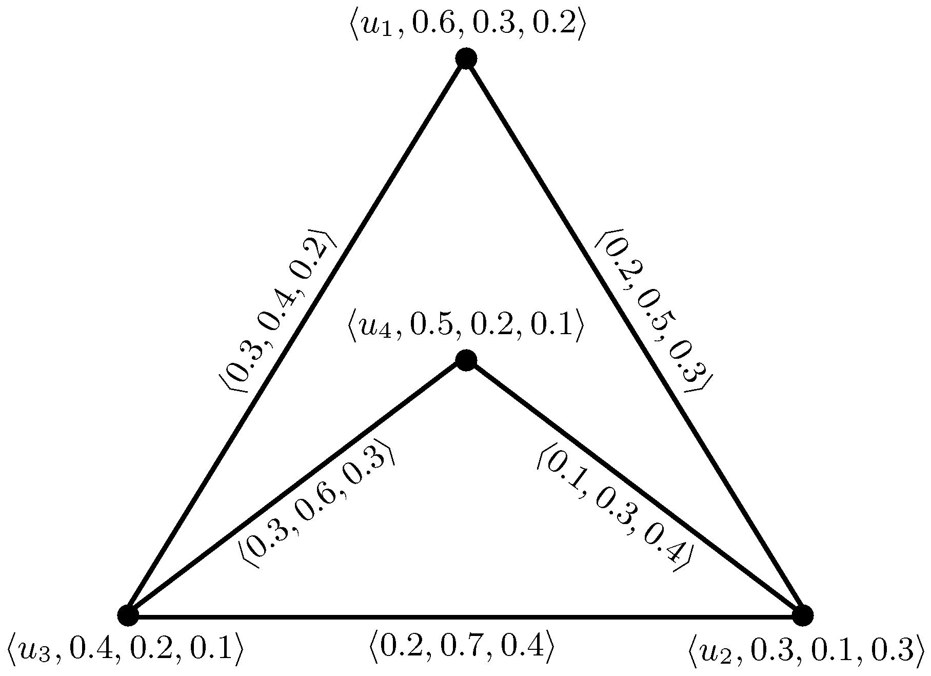
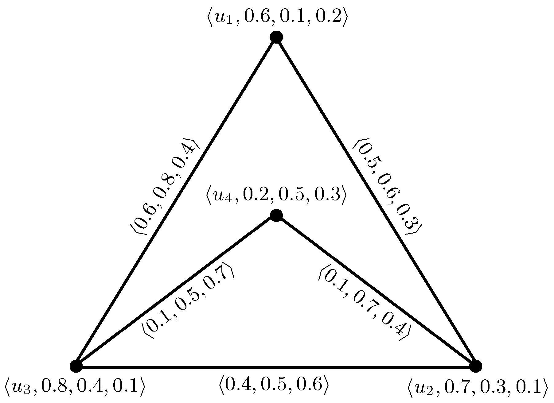
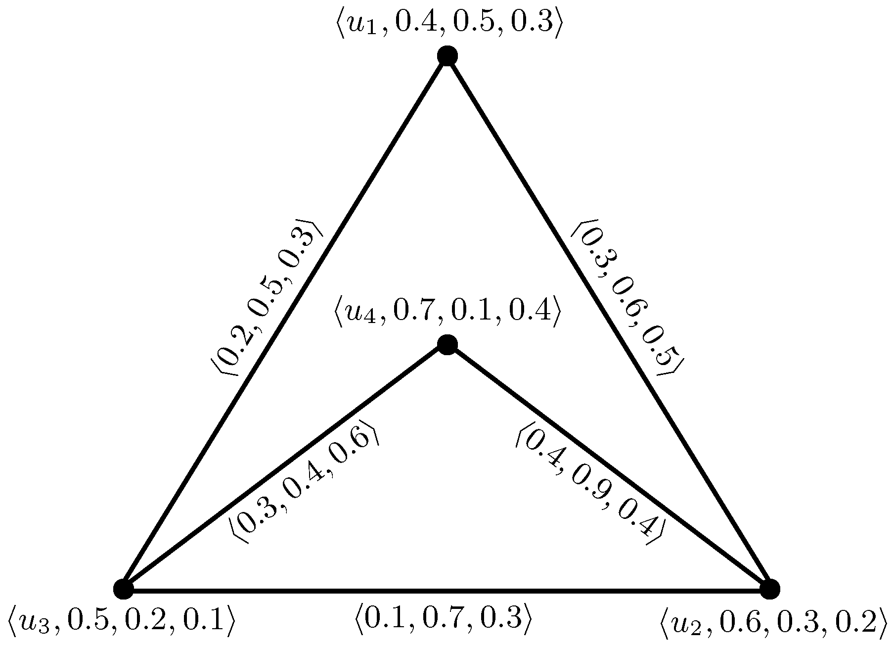
7. Real Time Example

In this section, the proposed concepts of energy, Laplacian energy and signless Laplacian energy of a SVNG are explained through a real time example. We have taken the Website http://www.pantechsolutions.net modeled as a SVNG by considering the navigation of the customer. We have taken the four links: 1. microcontroller-boards, 2. log-in html, 3. and 4. project kits for our calculation. A SVNG of this site for four different time periods is considered. The energy, Laplacian energy and signless Laplacian energy of a SVNG is calculated for each of these periods. The energy, Laplacian energy and signless Laplacian energy are represented in terms of bar graphs. In the website http://www.pantechsolutions.net (accessed on 8 May 2012). the above 4 links are considered for the period 16 January 2018 to 15 February 2018 and for this graph, as shown in Figure 9, we have

• Spec$(T_Y(u_j{u}_k))=\{-0.3442,-0.1000,0.0066,0.4376\}$,
• Spec$(I_Y(u_j{u}_k))=\{-0.6630,-0.2742,0.0774,0.8598\}$,
• Spec$(F_Y(u_j{u}_k))=\{-0.6703,-0.3296,0.0299,0.9701\}$,
• $E(T_Y(u_j{u}_k))=0.8884$, $E(I_Y(u_j{u}_k))=1.8744$, $E(F_Y(u_j{u}_k))=1.9999$.
• Therefore, $E({\mathcal{G}}_1)=\langle 0.8884,1.8744,1.9999\rangle .$

• Laplasian Spec$(T_Y(u_j{u}_k))=\{0,0.2492,0.5244,0.8264\}$,
• Laplacian Spec$(I_Y(u_j{u}_k))=\{0,0.6975,1.1757,1.5269\}$,
• Laplacian Spec$(F_Y(u_j{u}_k))=\{0,0.7605,1.4139,1.6256\}$,
• $LE(T_Y(u_j{u}_k))=1.1016$, $LE(I_Y(u_j{u}_k))=2.0051$, $LE(F_Y(u_j{u}_k))=2.2790$.
• Therefore, $LE({\mathcal{G}}_1)=\langle 1.1016,2.0051,2.2790\rangle .$

• Signless Laplacian Spec$(T_Y(u_j{u}_k))=\{-0.3183,-0.1339,-0.0555,0.5076\}$,
• Signless Laplacian Spec$(I_Y(u_j{u}_k))=\{-0.6764,-0.2500,0.0385,0.8879\}$,
• Signless Laplacian Spec$(F_Y(u_j{u}_k))=\{-0.7056,-0.2572,-0.0582,1.0211\}$,
• $L{E}^{+}(T_Y(u_j{u}_k))=1.0153$, $L{E}^{+}(I_Y(u_j{u}_k))=1.8529$, $L{E}^{+}(F_Y(u_j{u}_k))=2.0421$.
• Therefore, $L{E}^{+}({\mathcal{G}}_1)=\langle 1.0153,1.8529,2.0421\rangle .$

For the period 16 February 2018 to 15 March 2018 (see Figure 10), we have

• Spec$(T_Y(u_j{u}_k))=\{-0.4245,-0.1714,0.0215,0.5744\}$,
• Spec$(I_Y(u_j{u}_k))=\{-0.7909,-0.5799,0.0536,1.3173\}$,
• Spec$(F_Y(u_j{u}_k))=\{-0.5037,-0.3400,0.0007,0.8430\}$,
• $E(T_Y(u_j{u}_k))=1.1919$, $E(I_Y(u_j{u}_k))=2.7418$, $E(F_Y(u_j{u}_k))=1.6874$.
• Therefore, $E({\mathcal{G}}_2)=\langle 1.1919,2.7418,1.6874\rangle$.

• Laplacian Spec$(T_Y(u_j{u}_k))=\{0,0.4200,0.6908,1.0892\}$,
• Laplacian Spec$(I_Y(u_j{u}_k))=\{0,0.8716,1.7656,2.3629\}$,
• Laplacian Spec$(F_Y(u_j{u}_k))=\{0,0.5672,1.1546,1.4783\}$,
• $LE(T_Y(u_j{u}_k))=1.36$, $LE(I_Y(u_j{u}_k))=3.2569$, $LE(F_Y(u_j{u}_k))=2.0657$.
• Therefore, $LE\left({\mathcal{G}}_2\right)=\langle 1.36,3.2569,2.0657\rangle .$

• Signless Laplacian Spec$(T_Y(u_j{u}_k))=\{-0.4023,-0.1931,-0.0585,0.6538\}$,
• Signless Laplacian Spec$(I_Y(u_j{u}_k))=\{-0.7962,-0.5500,-0.1538,1.5000\}$,
• Signless Laplacian Spec$(F_Y(u_j{u}_k))=\{-0.5321,-0.2209,-0.2000,0.9530\}$,
• $L{E}^{+}(T_Y(u_j{u}_k))=1.3076$, $L{E}^{+}(I_Y(u_j{u}_k))=2.9999$, $L{E}^{+}(F_Y(u_j{u}_k))=1.9059$.
• Therefore, $L{E}^{+}({\mathcal{G}}_2)=\langle 1.3076,2.9999,1.9059\rangle .$

For the period 16 March 2018 to 15 April 2018 (see Figure 11), we have

• Spec$(T_Y(u_j{u}_k))=\{-0.6287,-0.3884,0.0004,1.0168\}$,
• Spec$(I_Y(u_j{u}_k))=\{-1.0779,-0.5696,0.0698,1.5776\}$,
• Spec$(F_Y(u_j{u}_k))=\{-0.8184,-0.4650,0.0051,1.2783\}$,
• $E(T_Y(u_j{u}_k))=2.0343$, $E(I_Y(u_j{u}_k))=3.2949$, $E(F_Y(u_j{u}_k))=2.5668.$
• Therefore, $E({\mathcal{G}}_3)=\langle 2.0343,3.2949,2.5668\rangle .$

• Laplacian Spec$(T_Y(u_j{u}_k))=\{0,0.2604,1.4221,1.7175\},$
• Laplacian Spec$(I_Y(u_j{u}_k))=\{0,1.2472,2.3360,2.6168\},$
• Laplacian Spec$(F_Y(u_j{u}_k))=\{0,0.8182,1.6721,2.3097\},$
• $LE(T_Y(u_j{u}_k))=2.8792$, $LE(I_Y(u_j{u}_k))=3.7056$, $LE(F_Y(u_j{u}_k))=3.1636$.
• Therefore, $LE({\mathcal{G}}_3)=\langle 2.8792,3.7056,3.1636\rangle$.

• Signless Laplacian Spec$(T_Y(u_j{u}_k))=\{-0.6816,-0.3513,-0.2007,1.2336\},$
• Signless Laplacian Spec$(I_Y(u_j{u}_k))=\{-1.1436,-0.4542,-0.0553,1.6531\},$
• Signless Laplacian Spec$(F_Y(u_j{u}_k))=\{-0.8066,-0.4000,-0.2632,1.4698\},$
• $L{E}^{+}(T_Y(u_j{u}_k))=2.4671$, $L{E}^{+}(I_Y(u_j{u}_k))=3.3062$, $L{E}^{+}(F_Y(u_j{u}_k))=2.9395$.
• Therefore, $L{E}^{+}({\mathcal{G}}_3)=\langle 2.4671,3.3062,2.9395\rangle$.

Finally, for the period 16 April 2018 to 15 May 2018 (see Figure 12), we have

• Spec$(T_Y(u_j{u}_k))=\{-0.5716,-0.0973,0.0027,0.6662\}$,
• Spec$(I_Y(u_j{u}_k))=\{-1.0878,-0.5755,0.0435,1.6198\}$,
• Spec$(F_Y(u_j{u}_k))=\{-0.7686,-0.3985,0.0990,1.0680\}$,
• $E(T_Y(u_j{u}_k))=1.3378$, $E(I_Y(u_j{u}_k))=3.3265$, $E(F_Y(u_j{u}_k))=2.3342$.
• Therefore, $E({\mathcal{G}}_4)=\langle 1.3378,3.3265,2.3342\rangle .$

• Laplacian Spec$(T_Y(u_j{u}_k))=\{0,0.5637,0.7641,1.2721\}$,
• Laplacian Spec$(I_Y(u_j{u}_k))=\{0,1.1660,2.0643,2.9697\}$,
• Laplacian Spec$(F_Y(u_j{u}_k))=\{0,0.8207,1.5544,1.8249\}$,
• $LE(T_Y(u_j{u}_k))=1.4725$, $LE(I_Y(u_j{u}_k))=3.868$, $LE(F_Y(u_j{u}_k))=2.5586$.
• Therefore, $LE({\mathcal{G}}_4)=\langle 1.4725,3.8680,2.5586\rangle .$

• Signless Laplacian Spec$(T_Y(u_j{u}_k))=\{-0.5588,-0.1017,-0.0500,0.7105\}$,
• Signless Laplacian Spec$(I_Y(u_j{u}_k))=\{-1.0582,-0.5617,-0.2105,1.8304\}$,
• Signless Laplacian Spec$(F_Y(u_j{u}_k))=\{-0.7996,-0.3562,0.0413,1.1145\}$,
• $L{E}^{+}(T_Y(u_j{u}_k))=1.4211$, $L{E}^{+}(I_Y(u_j{u}_k))=3.6608$, $L{E}^{+}(F_Y(u_j{u}_k))=2.3116$.
• Therefore, $L{E}^{+}({\mathcal{G}}_4)=\langle 1.4211,3.6608,2.3116\rangle .$

The bar graphs, shown in Figure 13, Figure 14 and Figure 15, represent the energy, Laplacian energy and signless Laplacian energy of four links for the above four periods corresponding to the truth-membership, indeterminacy-membership and falsity-membership values. From the above bar graphs, the energy, Laplacian energy and signless Laplacian energy of truth-membership for the period March to April is high as compared to other periods, the energy, Laplacian energy and signless Laplacian energy of indeterminacy-membership for the period April to May is high and, the energy, Laplacian energy and signless Laplacian energy of falsity-membership for the period March to April is high.

8. Conclusions

A single-valued neutrosophic model is used in computer technology, networking, communication, when the concept of indeterminacy is present. In this paper, we have introduced certain novel concepts, including energy, Laplacian energy and signless Laplacian energy of SVNGs. We have derived the lower and upper bounds for the energy and Laplacian energy of a SVNG. We have obtained the relations among energy, Laplacian energy and signless Laplacian energy of a SVNG. Among the properties of energy, Laplacian energy and signless Laplacian energy of a SVNG, there is a great deal of analogy, but also some significant differences. Finally, application in group decision-making based on SVNPRs is presented to illustrate the applicability of the proposed concepts of SVNGs. These concepts are also illustrated with real time example. We are planing to extend our research work to (1) Energy of bipolar neutrosophic graphs; (2) Simplified interval-valued Pythagorean fuzzy graphs; (3) Hesitant Pythagorean fuzzy graphs; Energy of neutrosophic hypergraphs.

References

1. Smarandache, F. A unifying field in logics. In Neutrosophy: Neutrosophic Probability, Set and Logic; American Research Press: Rehoboth, DE, USA, 1999. [Google Scholar]
2. Wang, H.; Smarandache, F.; Zhang, Y.Q.; Sunderraman, R. Single-valued neutrosophic sets. Multisp. Multistruct. 2010, 4, 410–413. [Google Scholar]
3. Atanassov, K.T. Intuitionistic fuzzy sets. Fuzzy Sets Syst. 1986, 20, 87–96. [Google Scholar]
4. Bhattacharya, S. Neutrosophic information fusion applied to the options market. Invest. Manag. Financ. Innov. 2005, 1, 139–145. [Google Scholar]
5. Aggarwal, S.; Biswas, R.; Ansari, A.Q. Neutrosophic modeling and control. In Proceedings of the 2010 International Conference on Computer and Communication Technology, Allahabad, India, 17–19 September 2010; pp. 718–723. [Google Scholar]
6. Guo, Y.; Cheng, H.D. New neutrosophic approach to image segmentation. Pattern Recognit. 2009, 42, 587–595. [Google Scholar]
7. Ye, J.; Fu, J. Multi-period medical diagnosis method using a single-valued neutrosophic similarity measure based on tangent function. Comput. Methods Programs Biomed. 2016, 123, 142–149. [Google Scholar]
8. Ye, J. Multicriteria decision-making method using the correlation coefficient under single-valued neutrosophic environment. Int. J. Gen. Syst. 2013, 42, 386–394. [Google Scholar]
9. Naz, S.; Rashmanlou, H.; Malik, M.A. Operations on single-valued neutrosophic graphs with application. J. Intell. Fuzzy Syst. 2017, 32, 2137–2151. [Google Scholar]
10. Ashraf, S.; Naz, S.; Rashmanlou, H.; Malik, M.A. Regularity of graphs in single-valued neutrosophic environment. J. Intell. Fuzzy Syst. 2017, 33, 529–542. [Google Scholar]
11. Gutman, I. The energy of a graph. Ber. Math. Stat. Sekt. Forsch. Graz. 1978, 103, 1–22. [Google Scholar]
12. Gutman, I. The Energy of a Graph: Old and New Results, Algebraic Combinatorics and Applications; Springer: Berlin/Heidelberg, Germany, 2001; pp. 196–211. [Google Scholar]
13. Gutman, I.; Zhou, B. Laplacian energy of a graph. In Linear Algebra and Its Applications; Elsevier: New York, NY, USA, 2006; Volume 414, pp. 29–37. [Google Scholar]
14. Gutman, I.; Robbiano, M.; Martins, E.A.; Cardoso, D.M.; Medina, L.; Rojo, O. Energy of line graphs. In Linear Algebra and Its Applications; Elsevier: New York, NY, USA, 2010; Volume 433, pp. 1312–1323. [Google Scholar]
15. Erdos, P. Graph theory and probability, canad. J. Math. 1959, 11, 34–38. [Google Scholar]
16. Zadeh, L.A. Fuzzy sets. Inf. Control 1965, 8, 338–353. [Google Scholar]
17. Kaufmann, A. Introduction a la Theorie des Sour-Ensembles Flous; Masson et Cie: Paris, France, 1973; p. 1. [Google Scholar]
18. Rosenfeld, A. Fuzzy Graphs, Fuzzy Sets and Their Applications; Zadeh, L.A., Fu, K.S., Shimura, M., Eds.; Academic Press: New York, NY, USA, 1975; pp. 77–95. [Google Scholar]
19. Anjali, N.; Mathew, S. Energy of a fuzzy graph. Ann. Fuzzy Maths Inform. 2013, 6, 455–465. [Google Scholar]
20. Sharbaf, S.R.; Fayazi, F. Laplacian energy of a fuzzy graph. Iran. J. Math. Chem. 2014, 5, 1–10. [Google Scholar]
21. Parvathi, R.; Karunambigai, M.G. Intuitionistic fuzzy graphs. In Computational Intelligence, Theory and Applications; Springer: Berlin/Heidelberg, Germany, 2006; pp. 139–150. [Google Scholar]
22. Akram, M. Bipolar fuzzy graphs. Inf. Sci. 2011, 181, 5548–5564. [Google Scholar]
23. Akram, M.; Davvaz, B. Strong intuitionistic fuzzy graphs. Filomat 2012, 26, 177–196. [Google Scholar]
24. Akram, M.; Malik, H.M.; Shahzadi, S.; Smarandache, F. Neutrosophic soft rough graphs with application. Axioms 2018, 7, 14. [Google Scholar]
25. Akram, M.; Siddique, S. Neutrosophic competition graphs with applications. J. Intell. Fuzzy Syst. 2017, 33, 921–935. [Google Scholar]
26. Akram, M.; Sitara, M.; Smarandache, F. Graph structures in bipolar neutrosophic environment. Mathematics 2017, 5, 60–80. [Google Scholar]
27. Naz, S.; Ashraf, S.; Akram, M. A novel approach to decision-making with Pythagorean fuzzy information. Mathematics 2018, 6, 1–28. [Google Scholar]
28. Ishfaq, N.; Sayed, S.; Akram, M.; Smarandache, F. Notions of rough neutrosophic digraphs. Mathematics 2018, 6, 18. [Google Scholar]
29. Sayed, S.; Ishfaq, N.; Akram, M.; Smarandache, F. Rough neutrosophic digraphs with application. Axioms 2018, 7, 5. [Google Scholar]
30. Akram, M.; Ishfaq, N.; Sayed, S.; Smarandache, F. Decision-making approach based on neutrosophic rough information. Algorithms 2018, 11, 59. [Google Scholar]
31. Naz, S.; Malik, M.A.; Rashmanlou, H. Hypergraphs and transversals of hypergraphs in interval-valued intuitionistic fuzzy setting. J. Mult.-Valued Logic Soft Comput. 2018, 30, 399–417. [Google Scholar]
32. Praba, B.; Chandrasekaran, V.M.; Deepa, G. Energy of an intutionistic fuzzy graph. Ital. J. Pure Appl. Math. 2014, 32, 431–444. [Google Scholar]
33. Basha, S.S.; Kartheek, E. Laplacian energy of an intuitionistic fuzzy graph. Ind. J. Sci. Technol. 2015, 8, 1–7. [Google Scholar]
34. Broumi, S.; Smarandache, F.; Talea, M.; Bakali, A. Single-valued neutrosophic graphs: degree, order and size. In Proceedings of the 2016 IEEE International Conference on Fuzzy Systems, Vancouver, BC, Canada, 24–29 July 2016; pp. 2444–2451. [Google Scholar]
35. Broumi, S.; Bakali, A.; Talea, M.; Smarandache, F.; Kishore, K.K.; Sahin, R. Shortest path problem under interval valued neutrosophic setting. J. Fundam. Appl. Sci. 2018, 10, 168–174. [Google Scholar]
36. Hamidi, M.; Saeid, A.B. Accessible single-valued neutrosophic graphs. J. Appl. Math. Comput. 2017, 1–26. [Google Scholar] [CrossRef]
37. Stanujkic, D.; Zavadskas, E.K.; Smarandache, F.; Brauers, W.K.; Karabasevic, D. A neutrosophic extension of the MULTIMOORA method. Informatica 2017, 28, 181–192. [Google Scholar]
38. Smarandache, F.; Ye, J. Summary of the Special Issue “Neutrosophic Information Theory and Applications” at “Information Journal”. Information 2018, 9, 49. [Google Scholar]
39. Tripathi, G. A matrix extension of the Cauchy-Schwarz inequality. Econ. Lett. 1999, 63, 1–3. [Google Scholar]
40. Akram, M.; Shahzadi, S. Neutrosophic soft graphs with application. J. Intell. Fuzzy Syst. 2017, 32, 841–858. [Google Scholar]
41. Fan, Z.P.; Liu, Y. An approach to solve group decision-making problems with ordinal interval numbers. IEEE Trans. Syst. Man Cybern. B Cybern. 2010, 40, 1413–1423. [Google Scholar]
42. Biswas, P.; Pramanik, S.; Giri, B.C. TOPSIS method for multi-attribute group decision-making under single-valued neutrosophic environment. Neural Comput. Appl. 2016, 27, 727–737. [Google Scholar]
Figure 1. Single-valued neutrosophic graph.
Axioms 07 00050 g001
Figure 2. Single-valued neutrosophic graph.
Axioms 07 00050 g002
Figure 3. Single-valued neutrosophic graph.
Axioms 07 00050 g003
Figure 4. Single-valued neutrosophic digraphs.
Axioms 07 00050 g004
Figure 5. Directed network of the fused SVNPR.
Axioms 07 00050 g005
Figure 6. Partial directed network of the fused SVNPR.
Axioms 07 00050 g006
Figure 7. Partial directed network of the fused SVNPR.
Axioms 07 00050 g007
Figure 8. Partial directed network of the fused SVNPR.
Axioms 07 00050 g008
Figure 9. Single-valued neutrosophic graph G 1 .
Axioms 07 00050 g009
Figure 10. Single-valued neutrosophic graph G 2 .
Axioms 07 00050 g010
Figure 11. Single-valued neutrosophic graph G 3 .
Axioms 07 00050 g011
Figure 12. Single-valued neutrosophic graph G 4 .
Axioms 07 00050 g012
Figure 13. Energy of single-valued neutrosophic graphs.
Axioms 07 00050 g013
Figure 14. Laplacian energy of single-valued neutrosophic graphs.
Axioms 07 00050 g014
Figure 15. Signless Laplacian energy of single-valued neutrosophic graphs.
Axioms 07 00050 g015