Collocation Methods for Volterra Integral and Integro-Differential Equations: A Review

Abstract

We present a collection of recent results on the numerical approximation of Volterra integral equations and integro-differential equations by means of collocation type methods, which are able to provide better balances between accuracy and stability demanding. We consider both exact and discretized one-step and multistep collocation methods, and illustrate main convergence results, making some comparisons in terms of accuracy and efficiency. Some numerical experiments complete the paper.

1. Introduction

It is the purpose of this paper to illustrate recent results on collocation methods for Volterra integral equations (VIEs) and Volterra integro-differential equations (VIDEs), mainly due to the authors. Such equations model evolutionary problems with memory in many applications, such as dynamics of viscoelastic materials with memory, electrodynamics with memory, heat conduction in materials with memory [1,2,3,4,5,6]. The numerical solution of these equations has a high computational cost due both to the nonlinearity of the advancing term and to the evaluation of the lag term, which contains the past history of the solution. Therefore, a crucial point is finding accurate and efficient numerical methods.

Collocation methods have several desirable properties. They provide an approximation over the entire integration interval to the solution of the equation, which reveals to be quite useful in a variable-stepsize implementation: indeed, it is easy to recover the missing past values when the stepsize is changed, by evaluating the collocation polynomial. Other good properties of collocation methods are their high order of convergence, strong stability properties and flexibility. As a matter of fact, if some information is known on the behavior of the exact solution, then it is possible to choose the collocation functions in order to better follow such behavior, so giving rise to mixed collocation methods, see for example [7] in the case of ordinary differential equations (ODEs), and [8] in the case of VIEs. It is also worthwhile mentioning that collocation also has an important theoretical relevance: in fact, many numerical methods are difficult to be analyzed as discrete schemes while, re-casted as collocation-based methods, their analysis is reasonably simplified and can be carried out in a very elegant way. There is, however, a remarkable drawback of one-step collocation methods: they suffer from order reduction phenomenon when applied to stiff problems [9,10,11], since the order of convergence is not uniform (for instance, in the case of s-stage collocation based Runge-Kutta methods on Gauss-Legendre collocation points, the order is $p=2s$ in the grid points, but it degenerates to $p=s$ for stiff problems, since the order is s in the internal stages). Such a drawback is successfully solved by two-step collocation methods [12], having high uniform order on the overall integration interval. On the side of computational cost, collocation methods are usually more expensive than other classes of methods. In fact, a collocation method with m collocation parameters requires at each time-step the solution of a nonlinear system of dimension m. To face this drawback, multistep collocation methods can be adopted which increase the order of convergence at the same computational cost of one-step ones. When a collocation method is applied to an integral equation, several integrals must be computed, thus suitable quadrature rules are needed to complete the discretization, with the introduction of an additional error. Lastly, a reliable error estimation for collocation methods for integral equations is still missing: there have been some advances (compare [13] and references therein contained), however considerable work needs to be done.

One-step collocation methods first appeared in the literature and main results are collected in the monographs [2,3]. Recently, we have proposed multistep collocation methods [13,14,15,16] and two step almost collocation methods [13,17,18], where the collocation polynomial depends on the approximate solution in a fixed number of previous time steps, with the aim of increasing the order of convergence of classical one–step collocation methods, without additional computational cost at each time step, and at the same time obtaining highly stable methods. This idea has been already proposed for the numerical solution of ODEs [19,20,21] (see also [11], Section V.3), and afterward modified in [12], by also using the inherent quadratic technique [22,23,24]. We also underline that they have high uniform order, thus they do not suffer from the order reduction phenomenon, well-known in the ODEs context [9]. Other approaches, based on multistep collocation, have been proposed in [25,26,27,28,29,30,31,32].

Here we briefly introduce one-step collocation methods and illustrate with more detail the construction and analysis of multistep collocation methods for VIEs and VIDEs, with the aim of giving a complete idea on the recent developments in this context. We give practical indications on how to choose the quadrature formulas in the discretized methods for an efficient implementation. In this review, we consider VIEs and VIDEs with smooth kernel and solution. We illustrate methods with a uniform mesh, however they could easily be applied to a non-uniform mesh (compare [2] for one-step collocation methods).

The paper is organized as follows. Section 2 and Section 3 deal with one-step and multistep collocation methods for VIEs, respectively. Section 4 illustrates two-step almost collocation methods for VIEs. Section 5 and Section 6 focus on one-step and multistep collocation methods for VIDEs, respectively.

2. One Step Collocation Methods for VIES

We consider VIEs of the form

$$y(t)=g(t)+{\int }_0^{t}k(t,\tau ,y(\tau ))d\tau ,t\in I=[0,T],$$

(1)

where $k\in C(D\times \mathbb{R})$, with $D:=\left\{(t,\tau ):0\le \tau \le t\le T\right\}$, and $g\in C(I)$. In the literature, many authors (see [2,3] and references therein contained) have analyzed one step collocation methods for VIEs. As it is well known, a collocation method is based on the idea of approximating the exact solution of a given integral equation with a suitable function belonging to a chosen finite dimensional space, usually a piecewise algebraic polynomial which satisfies the integral equation exactly on a certain subset of the integration interval (called the set of collocation points).

Let us discretize the interval I by introducing a uniform mesh

$$I_h=\left\{t_n:=nh,n=0,\dots ,N,\right.\left.h\ge 0,Nh=T\right\}.$$

The Equation (1) can be rewritten, by relating it to this mesh, as

$$\begin{array}{cc}y(t)=F_n(t)+{\mathsf{\Phi }}_n(t)& t\in [t_n,t_{n+1}],\end{array}$$

where

$$F_n(t):=g(t)+{\displaystyle {\int }_0^{t_n}}k(t,\tau ,y(\tau ))d\tau$$

and

$${\mathsf{\Phi }}_n(t):={\displaystyle {\int }_{t_n}^t}k(t,\tau ,y(\tau ))d\tau$$

represent respectively the lag term and the increment function.

Collocation methods provide an approximation $P(t)$ to the solution $y(t)$ of (1) on $[0,T]$, such that its restriction to each interval $(t_n,t_{n+1}]$ is a polynomial:

$${P(t)|}_{(t_n,t_{n+1}]}=P_n(t).$$

2.1. Exact One-Step Collocation Methods

Let us fix m collocation parameters $0\le c_1<\dots <c_m\le 1$ and denote by $t_{nj}=t_n+c_{j}h$ the collocation points. The collocation polynomial, restricted to the interval $[t_n,t_{n+1}]$, is of the form:

$$P_n(t_n+sh)=\sum _{j=1}^m{L}_j(s)Y_{nj}s\in [0,1]n=0,\dots ,N-1$$

(2)

where $L_j(s)$ is the j-th Lagrange fundamental polynomial with respect to the collocation parameters and $Y_{nj}:=P_n(t_{nj})$. Exact collocation methods are obtained by imposing that the collocation polynomial (2) exactly satisfies the VIE (1) in the collocation points $t_{n,i}$ and by computing $y_{n+1}=P_n(t_{n+1})$:

$$\left\{\begin{array}{c}{Y}_{ni}=F_{ni}+{\mathsf{\Phi }}_{ni}\\ y_{n+1}={\displaystyle \sum _{j=1}^m}{L}_j(1)Y_{nj}\end{array}\right.,$$

(3)

where

$$F_{ni}=g(t_{ni})+h\sum _{\nu =0}^{n-1}{\displaystyle {\int }_0^1}k(t_{ni},t_{\nu }+sh,P_{\nu }(t_{\nu }+sh))ds$$

(4)

$${\mathsf{\Phi }}_{ni}=h{\displaystyle {\int }_0^{c_i}}k(t_{ni},t_n+sh,P_n(t_n+sh))ds,$$

(5)

$i=1,\dots ,m$. Note that the first equation in (3) represents a system of m nonlinear equations in the m unknowns $Y_{ni}$. We recall that generally $P(t)$ is not continuous in the mesh points, as

$$P(t)\in S_{m-1}^{(-1)}(I_h),$$

(6)

where

$$\begin{array}{c}\hfill S_{\mu }^{(d)}(I_h)=\left\{v\in C^d(I):{\left.v\right|}_{(t_n,t_{n+1}]}\in {\Pi }_{\mu },n=0,1,\dots ,N-1\right\}.\end{array}$$

Here, ${\Pi }_{\mu }$ denotes the space of (real) polynomials of degree not exceeding $\mu$.

The classical collocation methods have uniform order $O(h^m)$ for any choice of the collocation parameters, and can achieve local superconvergence in the mesh points by opportunely choosing the collocation parameters, i.e., order $2m-2$ with m Lobatto points or $m-1$ Gauss points with $c_m=1$ and order $2m-1$ with m Radau II points. The optimal superconvergence order $O(h^{2m})$ in the mesh points can be achieved with Gauss nodes in the iterated collocation methods [2,3].

2.2. Discretized One-Step Collocation Methods

The collocation Equation (3) is not yet in a form amenable to numerical computation: another discretization step, based on quadrature formulas ${\tilde{F}}_{ni}\simeq F_{ni}$ and ${\tilde{\mathsf{\Phi }}}_{ni}\simeq {\mathsf{\Phi }}_{ni}$ for the approximation of (4) and (5) are needed in order to obtain the fully discretised collocation schemes, thus leading to Discretized collocation methods.

The discretized collocation polynomial is of the form

$${\tilde{P}}_n(t_n+sh)=\sum _{j=1}^m{L}_j(s){\tilde{Y}}_{nj}s\in [0,1]n=0,\dots ,N-1$$

(7)

where ${\tilde{Y}}_{nj}:={\tilde{P}}_n(t_{nj})$. The m unknowns ${\tilde{Y}}_{nj}$ are determined by imposing that the collocation polynomial (7) satisfies exactly the integral equation at the collocation points and by using quadrature formulas of the form

$${\tilde{\mathsf{\Phi }}}_n(t_{ni})=h\sum _{l=0}^{{\mu }_0}{w}_{il}k(t_{ni},t_n+d_{il}h,{\tilde{P}}_n(t_n+d_{il}h))$$

(8)

$${\tilde{F}}_n(t_{ni})=g(t_{ni})+h\sum _{\nu =0}^{n-1}\sum _{l=0}^{{\mu }_1}{b}_{l}k(t_{ni},t_{\nu }+{\xi }_{l}h,{\tilde{P}}_{\nu }(t_{\nu }+{\xi }_{l}h)),$$

(9)

$i=1,\dots ,m$, for approximating the lag term (4) and the increment function (5). The Formulas (8) and (9) are obtained by using quadrature formulas of the form

$${({\xi }_l,b_l)}_{l=1}^{{\mu }_1},{(d_{il},w_{il})}_{l=1}^{{\mu }_0},i=1,\dots ,m,$$

(10)

where the quadrature nodes ${\xi }_l$ and $d_{il}$ satisfy $0\le {\xi }_1<\dots <{\xi }_{{\mu }_1}\le 1$ and $0\le d_{i1}<\dots <d_{i{\mu }_0}\le 1$, ${\mu }_0$ and ${\mu }_1$ are positive integers and $w_{il}$, $b_l$ are suitable weights.

The numerical method is then of the form:

$$\left\{\begin{array}{c}{\tilde{Y}}_{ni}={\tilde{F}}_n(t_{ni})+{\tilde{\mathsf{\Phi }}}_n(t_{ni})\\ {\tilde{y}}_{n+1}={\displaystyle \sum _{j=1}^m}{L}_j(1){\tilde{Y}}_{nj}\end{array}\right.,$$

(11)

where ${\tilde{\mathsf{\Phi }}}_n(t_{ni})$ and ${\tilde{F}}_n(t_{ni})$ are given by (8) and (9).

Note that the first equation in (9) represents a system of m nonlinear equations in the m unknowns ${\tilde{Y}}_{ni}$.

Such methods preserve, under suitable hypothesis on the quadrature Formulas (8) and (9), the same order of the exact collocation methods [3].

A collocation method for VIEs is equivalent to an implicit Runge-Kutta method for VIEs (VRK method) if and only if $c_m=1$ (see Theorem 5.2.2 of [3]). As the lag–term computation is the most expensive part in the numerical solution of VIEs, fast collocation and Runge–Kutta methods have been constructed for convolution VIEs of Hammerstein type [33,34] in order to reduce the computational effort in the lag–term computation. The stability analysis of collocation methods for VIEs can be found in [3,35] and the related bibliography.

3. Multistep Collocation Methods for VIEs

Multistep collocation methods for VIEs have been introduced in [16] by adding interpolation conditions in r previous step points, with the aim of increasing the uniform order of convergence of one step collocation methods without increasing the computational cost. The multistep collocation polynomial, restricted to the interval $[t_n,t_{n+1}]$, is of the form

$$P_n(t_n+sh)=\sum _{k=0}^{r-1}{\phi }_k(s)y_{n-k}+\sum _{j=1}^m{\psi }_j(s)Y_{nj}s\in [0,1],$$

(12)

$n=r,\dots ,N-1$, where again

$$Y_{nj}:=P_n(t_{nj})$$

(13)

and ${\phi }_k(s)$, ${\psi }_j(s)$ are the following polynomials of degree $m+r-1$

$${\phi }_k(s)=\prod _{i=1}^m\frac{s-c_i}{-k-c_i}·\prod _{\begin{array}{c}i=0\\ i\ne k\end{array}}^{r-1}\frac{s+i}{-k+i},{\psi }_j(s)=\prod _{i=0}^{r-1}\frac{s+i}{c_j+i}·\prod _{\begin{array}{c}i=1\\ i\ne j\end{array}}^m\frac{s-c_i}{c_j-c_i}.$$

(14)

The collocation parameters are assumed to satisfy $c_i\ne c_j$ and $c_1\ne 0$.

3.1. Exact Multistep Collocation

The exact multistep collocation methods are obtained by imposing that the collocation polynomial (12) exactly satisfies the VIE (1) at the collocation points $t_{ni}$, and by computing $y_{n+1}=P_n(t_{n+1})$:

$$\left\{\begin{array}{c}{Y}_{ni}=F_{ni}+{\mathsf{\Phi }}_{ni},\\ y_{n+1}={\displaystyle \sum _{k=0}^{r-1}}{\phi }_k(1)y_{n-k}+{\displaystyle \sum _{j=1}^m}{\psi }_j(1)Y_{nj},\end{array}\right.$$

(15)

where the lag–term $F_{ni}$ and increment–term ${\mathsf{\Phi }}_{ni}$ are given by (4) and (5) respectively. The r-step m-point exact collocation method (12)–(15) has uniform convergence order of at least $p=m+r$, for any choice of distinct collocation abscissas $0<c_1<\dots <c_m\le 1$, as stated in the following theorem proved in [16].

Theorem 1.

Let $\epsilon (t)=y(t)-P(t)$ be the error of the exact collocation method (12)–(15) and $p=m+r$. Suppose that

i. 

the given functions describing the VIE (1) satisfy $k\in C^{(p)}(D\times \mathbb{R})$, $g\in C^{(p)}(I)$.

ii. 

the starting error is ${∥\epsilon ∥}_{\infty ,[0,t_r]}=O(h^p)$.

iii. 

$\rho (\mathbf{A})<1$, where

$$\mathbf{A}=\left[\begin{array}{cc}\hfill [c]c|c{\mathbf{0}}_{r-1,1}& {\mathbf{I}}_{r-1}\\ \hfill {\phi }_{r-1}(1)& {\phi }_{r-2}(1),\dots ,{\phi }_0(1)\end{array}\right]$$

(16)

and ρ denotes the spectral radius.

Then

$${∥\epsilon ∥}_{\infty }=O(h^{m+r}).$$

Moreover, a suitable choice of collocation parameters can ensure superconvergence in the mesh points, as pointed out in the following theorem [16].

Theorem 2.

Let us suppose that

• the hypothesis of the Theorem 1 hold with $p=2m+r-1$.
• the collocation parameters $c_1,\dots ,c_m$ are the solution of the system

  $$\left\{\begin{array}{c}{c}_m=1\hfill \\ \frac{1}{i+1}-{\displaystyle \sum _{k=0}^{r-1}}{\beta }_k{(-k)}^i-{\displaystyle \sum _{j=1}^m}{\gamma }_j{(c_j)}^i=0,i=m+r,...,2m+r-2\hfill \end{array}\right.$$

  (17)

  with

  $${\beta }_k={\int }_0^1{\phi }_k(s)ds,{\gamma }_j={\int }_0^1{\psi }_j(s)ds$$

  (18)

then

$$\underset{n=0,\dots ,N}{max}\left|\epsilon (t_n)\right|=O(h^{2m+r-1}).$$

3.2. Discretized Multistep Collocation

The discretized multistep collocation methods are obtained by using quadrature formulas of the form (8) to (9) for approximating the lag term and the increment function. The discretized multistep collocation polynomial, denoted by ${\tilde{P}}_n(t)$, is then of the form

$${\tilde{P}}_n(t_n+sh)=\sum _{k=0}^{r-1}{\phi }_k(s){\tilde{y}}_{n-k}+\sum _{j=1}^m{\psi }_j(s){\tilde{Y}}_{nj},s\in [0,1]$$

(19)

$n=0,\dots ,N-1$,where the functions ${\phi }_k(s)$ and ${\psi }_j(s)$ are given by (14), and ${\tilde{Y}}_{nj}:={\tilde{P}}_n(t_{nj})$ are determined by the solution of the following nonlinear system

$$\left\{\begin{array}{cc}{\tilde{Y}}_{ni}=\hfill & {\tilde{F}}_{ni}+{\tilde{\mathsf{\Phi }}}_{ni},\hfill \\ {\tilde{y}}_{n+1}=\hfill & {\displaystyle \sum _{k=0}^{r-1}}{\phi }_k(1){\tilde{y}}_{n-k}+{\displaystyle \sum _{j=1}^m}{\psi }_j(1){\tilde{Y}}_{nj}.\hfill \end{array}\right.$$

(20)

The following theorem [16] shows that, as in the exact case, the r-step m-point discretized collocation method (19) and (20) has convergence order of at least $p=m+r$, for any choice of distinct collocation abscissas $0<c_1<\dots <c_m\le 1$.

Theorem 3.

Let $\tilde{\epsilon }(t):=y(t)-\tilde{P}(t)$ be the error of the discretized collocation method (19) and (20) and let $p=m+r$. Suppose that

i. 

the given functions describing the VIE (1) satisfy $k\in C^{(p)}(D)$, $g\in C^{(p)}(I)$;

ii. 

the lag–term and increment–term quadrature Formulas (10) are of order respectively at least $p+1$ and p;

iii. 

the starting error is ${∥\tilde{\epsilon }∥}_{\infty ,[0,t_r]}=O(h^p)$.

iv. 

$\rho (\mathbf{A})<1$, where A is given by (16).

Then

$${∥\tilde{\epsilon }∥}_{\infty }=O(h^{m+r}).$$

An analogous result holds concerning the local superconvergence:

Theorem 4.

Let us suppose that

• the hypothesis of the Theorem 3 hold with $p=2m+r-1$.
• the collocation parameters $c_1,\dots ,c_m$ are the solution of the system (17).

Then

$$\underset{n=0,\dots ,N}{max}\left|\tilde{\epsilon }(t_n)\right|=O(h^{2m+r-1}).$$

4. Two Step Almost Collocation Collocation Methods for VIEs

Within the class of multistep collocation methods, although methods with unbounded stability regions exist, no A-stable methods have been found [16]. In order to determine A-stable methods, two step almost collocation (TSAC) methods have been introduced in [18] and further analyzed in [13,17].

The collocation polynomial $P_n(t)$ for TSAC methods is computed by employing the information about the equation on two consecutive steps:

$$P_n(t_n+sh)={\phi }_0(s)y_{n-1}+{\phi }_1(s)y_n+\sum _{j=1}^m{\chi }_j(s)Y_j^{[n]}+\sum _{j=1}^m{\psi }_j(s)(F_j^{[n]}+{\mathsf{\Phi }}_j^{[n+1]}),$$

(21)

where $Y_j^{[n]}=P(t_{n-1,j})$. Then the method assumes the form:

$$\left\{\begin{array}{cc}\hfill Y_i^{[n+1]}& {\displaystyle ={\phi }_0(c_i)y_{n-1}+{\phi }_1(c_i)y_n+{\displaystyle \sum _{j=1}^m}{\chi }_j(c_i)Y_j^{[n]}+{\displaystyle \sum _{j=1}^m}{\psi }_j(c_i)\left(F_j^{[n]}+{\mathsf{\Phi }}_j^{[n+1]}\right),}\hfill \\ \hfill y_{n+1}& {\displaystyle ={\phi }_0(1)y_{n-1}+{\phi }_1(1)y_n+{\displaystyle \sum _{j=1}^m}{\chi }_j(1)Y_j^{[n]}+{\displaystyle \sum _{j=1}^m}{\psi }_j(1)\left(F_j^{[n]}+{\mathsf{\Phi }}_j^{[n+1]}\right),}\hfill \end{array}\right.$$

(22)

where $F_j^{[n]}$ and ${\mathsf{\Phi }}_j^{[n+1]}$ are suitable sufficiently high order quadrature formulae for the discretization of $F^{[n]}(t_{nj})$ and ${\mathsf{\Phi }}^{[n+1]}(t_{nj})$ respectively, assuming the form

$$F_j^{[n]}=g(t_{nj})+h\sum _{\nu =1}^n\sum _{l=0}^{m+1}{b}_{l}k\left(t_{nj},t_{\nu -1,l},Y_l^{[\nu ]}\right),$$

(23)

and

$${\mathsf{\Phi }}_j^{[n+1]}=h\sum _{l=0}^{m+1}{w}_{jl}k\left(t_{nj},t_{nl},Y_l^{[n+1]}\right).$$

(24)

In the quadrature Formulas (23) and (24) we mean $t_{\nu -1,0}=t_{\nu -1}$, $t_{\nu -1,m+1}=t_{\nu }$, $Y_0^{[\nu ]}=P_n(t_{\nu -1})$, $Y_{m+1}^{[\nu ]}=P_n(t_{\nu })$ and $t_{n0}=t_n$. We observe as the method (22) requires, at each step, the solution of a nonlinear system of $(m+1)d$ equations in the stage values $Y_i^{[n+1]}$ and $y_{n+1}$.

The basis functions ${\phi }_0(s)$, ${\phi }_1(s)$, ${\chi }_j(s)$ and ${\psi }_j(s)$, $j=1,2,\dots ,m$, are polynomials of degree p, determined from the continuous order conditions, according to the following theorem [18]:

Theorem 5.

Assume that the kernel $k(t,\eta ,y)$ and the function $g(t)$ in (1) are sufficiently smooth. Then the method (21) and (22) has uniform order p, i.e.,

$$\eta (t_n+sh)=O(h^{p+1}),h\to 0,$$

for $s\in [0,1]$, if the polynomials ${\phi }_0(s),$ ${\phi }_1(s),$ ${\chi }_j(s)$ and ${\psi }_j(s),$ $j=1,2,\dots ,m$ satisfy the system of equations

$$\left\{\begin{array}{cc}\hfill 1& {\displaystyle -{\phi }_0(s)-{\phi }_1(s)-{\displaystyle \sum _{j=1}^m}{\chi }_j(s)-{\displaystyle \sum _{j=1}^m}{\psi }_j(s)=0,}\hfill \\ \hfill s^k& {\displaystyle -{(-1)}^k{\phi }_0(s)-{\displaystyle \sum _{j=1}^m}{(c_j-1)}^k{\chi }_j(s)-{\displaystyle \sum _{j=1}^m}{c}_j^k{\psi }_j(s)=0,}\hfill \end{array}\right.$$

(25)

$s\in [0,1]$, $k=1,2,\dots ,p$, where

$${\displaystyle \eta (t_n+sh)=y(t_n+sh)-{\phi }_0(s)y(t_n-h)-{\phi }_1(s)y(t_n)-\sum _{j=1}^m\left({\chi }_j(s)y(t_n+(c_j-1)h)+{\psi }_j(s)y(t_n+c_{j}h)\right).}$$

(26)

is the local truncation error.

As regards the global error, the method has uniform order of convergence $p^{*}=min\{l+1,q,p+1\}$, where l and q are the order of the starting procedure (for the computation of the starting values $y_1$ and $Y_i^{[1]}$, $i=1,2,\dots ,m$) and the order of the quadrature Formulas (23) and (24) respectively (see Theorem 2.5 in [18]). Then we use as starting procedure a one step collocation method having uniform order of convergence $l=p$.

Two-step collocation methods are obtained by solving the system of order conditions up to the maximum uniform attainable order $p=2m+1$, and, in this way, all the basis functions are determined as the unique solution of such system. However, as observed in [18], it is not convenient to impose all the order conditions because it is not possible to achieve high stability properties (e.g., A-stability) without getting rid of some of them. Therefore, almost collocation methods have been introduced by relaxing a specified number r of order conditions, i.e., by a priori opportunely fixing r basis functions, and determining the remaining ones as the unique solution of the system of order conditions up to $p=2m+1-r$. Within the class of TSAC methods, A-stable methods have been constructed in [18] by fixing one (case $r=1$) or both (case $r=2$) of the polynomials ${\phi }_0(s)$ and ${\phi }_1(s)$ as

$$\begin{array}{c}{\displaystyle {\phi }_0(s)=\prod _{k=1}^m(s-c_k)(q_0+q_{1}s+\dots +q_{p-m}{s}^{p-m}),}\hfill \\ {\displaystyle {\phi }_1(s)=\prod _{k=1}^m(s-c_k)(p_0+p_{1}s+\dots +p_{p-m}{s}^{p-m}),}\hfill \end{array}$$

(27)

where ${\alpha }_j$ and ${\beta }_j$, $j=0,1,\dots ,p-m$, are free parameters, which have to be determined in order to obtain desired stability properties.

A error estimation of the local discretization error for TSAC methods has been derived in [13].

Example 1.

Let us consider the methods with two stages $m=2$ and order $p=2m=4$. Classes of A-stable methods were derived in [13,18] by considering

$${\phi }_0(s)=s(s-c_1)(s-c_2)(q_0+q_{1}s),$$

where $c_1$, $c_2$, $q_0$, $q_1$ are free parameters. The weights in (23) and (24) were computed in [18] as

$$\mathbf{b}=\left[\begin{array}{c}\hfill \frac{-1+2c_1+2c_2-6c_1{c}_2}{12c_1{c}_2}\\ \hfill \frac{1-2c_2}{12c_1(c_1-1)(c_1-c_2)}\\ \hfill \frac{2c_1-1}{12c_2(c_2-1)(c_2-c_1)}\\ \hfill \frac{-3+4c_1+4c_2-6c_1{c}_2}{12(c_1-1)(c_2-1)}\end{array}\right],\mathbf{W}=\left[\begin{array}{cccc}-\frac{c_1^2-3c_1{c}_2}{6c_2}& \frac{c_1(2c_1-3c_2)}{6(c_1-c_2)}& \frac{c_1^3}{6c_2(c_1-c_2)}& 0\\ -\frac{c_2^2-3c_1{c}_2}{6c_1}& -\frac{c_1^3}{6c_1(c_1-c_2)}& -\frac{c_2(2c_2-3c_1)}{6(c_1-c_2)}& 0\end{array}\right].$$

An A-stable method is obtained by choosing for example $q_0=15/10$, $q_1=-1$, $c_1=0.9$, $c_2=0.95$, see [13].

4.1. Diagonally Implicit TSAC Methods for VIEs

The computational cost associated to the solution of the nonlinear system (22) can be reduced by making the coefficient matrix have a structured shape, e.g., lower triangular or diagonal. This strategy, in the field of Runge–Kutta methods for ODEs, leads to the raise of the famous classes of Diagonally Implicit and Singly Diagonally Implicit Runge-Kutta methods (DIRK and SDIRK), see [10,11] and bibliography therein contained. Moreover, in the field of collocation-based methods for ODEs, an analogous strategy has been applied, obtaining TSAC methods having structured coefficient matrix [12].

In fact, a lower triangular matrix allows to solve the equations in m successive stages, with only a d-dimensional system to be solved at each stage. Moreover, if all the elements on the diagonal are equal, in solving the nonlinear systems by means of Newton-type iterations, one may hope to use repeatedly the stored $LU$ factorization of the Jacobian. If the structure is diagonal, the problem reduces to the solution of m independent systems of dimension d, and can therefore be solved in a parallel environment.

Methods of this type have been derived in [17], where first of all it was assumed $w_{j,m+1}=0$, $j=1,\dots ,m$, in such a way that (22) becomes a nonlinear system of dimension $md$ only depending on the stage values $Y_i^{[n+1]}$, $i=1,\dots ,m$, and assumes the following form

$$\left\{\begin{array}{c}{\displaystyle Y_i^{[n+1]}-h\sum _{j=1}^m\sum _{l=1}^m{\psi }_j(c_i)w_{jl}k(t_{nj},t_{nl},Y_l^{[n+1]})=B_i^{[n]},}\hfill \\ y_{n+1}=P_n(t_{n+1}),\hfill \end{array}\right.$$

(28)

where

$$B_i^{[n]}={\phi }_0(c_i)y_{n-1}+{\phi }_1(c_i)y_n+\sum _{j=1}^m{\chi }_j(c_i)Y_j^{[n]}+\sum _{j=1}^m{\psi }_j(c_i)F_j^{[n]}+h\sum _{j=1}^m{\psi }_j(c_i)w_{j0}k(t_{nj},t_n,y_n).$$

(29)

By defining

$$Y^{[n+1]}={\left[Y_1^{[n+1]},Y_2^{[n+1]},\dots ,Y_m^{[n+1]}\right]}^T,B^{[n]}={\left[B_1^{[n]},B_2^{[n]},\dots ,B_m^{[n]}\right]}^T,\mathsf{\Psi }={\left({\psi }_j(c_i)\right)}_{i,j=1}^m,$$

$$W={\left(w_{jl}\right)}_{j,l=1}^m,K(t_{nc},t_{nc},Y^{[n+1]})={\left(K(t_{ni},t_{nj},Y_j^{[n+1]})\right)}_{i,j=1}^m,$$

the nonlinear system in (28) takes the form

$$Y^{[n+1]}-h(\mathsf{\Psi }\otimes I)\left((W\otimes I)·K(t_{nc},t_{nc},Y^{[n+1]})\right)e=B^{[n]},$$

(30)

where · denotes the usual Hadamard product, I is the identity matrix of dimension d and e is the unit vector of dimension $md$. The tensor form (30) clearly shows as the matrices which determine the structure of the nonlinear system (28) are $\mathsf{\Psi }$ and W. In [17] a strategy was described to obtain lower triangular or diagonal structures for the matrices $\mathsf{\Psi }$ and W: in particular a quadrature formula of the form

$$\underset{0}{\overset{c_j}{\int }}f(s)ds\approx w_{j0}f(0)+\sum _{l=1}^m{\tilde{w}}_{jl}f(c_l-1)+\sum _{l=1}^j{w}_{jl}f(c_l),$$

(31)

was proposed for the increment

$${\displaystyle {\mathsf{\Phi }}^{[n+1]}(t_{nj},P(·))=h\underset{0}{\overset{c_j}{\int }}k(t_{nj},t_n+sh,P_n(t_n+sh))ds,}$$

(32)

in addition to the quadrature formula

$$\underset{0}{\overset{1}{\int }}f(s)ds\approx b_{0}f(0)+\sum _{l=1}^m{b}_{l}f(c_l)+b_{m+1}f(1),$$

(33)

for the approximation of the lag term

$${\displaystyle F^{[n]}(t_{nj},P(·))=g(t_{nj})+h\sum _{\nu =1}^n\underset{0}{\overset{1}{\int }}k(t_{nj},t_{\nu -1}+sh,P_{\nu -1}(t_{\nu -1}+sh))ds.}$$

(34)

We observe that in Formula (31), in case of triangular structure, ${\tilde{w}}_{jl}=0$, $l=1,\dots ,j$ while, in case of diagonal structure, ${\tilde{w}}_{j1}=0$ and $w_{jl}=0$, $l=1,\dots ,j-1$. The determination of the weights in Formulas (31) and (33) has been described in [17].

Assuming that $\mathsf{\Psi }$ and W are lower triangular, we obtain the diagonally implicit TSAC methods (DITSAC)

$$\left\{\begin{array}{cc}\hfill Y_i^{[n+1]}& -h{\psi }_i(c_i)w_{ii}k(t_{ni},t_{ni},Y_i^{[n+1]})=B_i^{[n]}+{\tilde{B}}_i^{[n]}+h\sum _{l=1}^{i-1}\sum _{j=l}^i{\psi }_j(c_i)w_{jl}k(t_{nj},t_{nl},Y_l^{[n+1]}),\hfill \\ \hfill y_{n+1}& {\displaystyle ={\phi }_0(1)y_{n-1}+{\phi }_1(1)y_n+\sum _{j=1}^m{\chi }_j(1)Y_j^{[n]}+\sum _{j=1}^m{\psi }_j(1)\left(F_j^{[n]}+{\mathsf{\Phi }}_j^{[n+1]}\right),}\hfill \end{array}\right.$$

(35)

where $B_i^{[n]}$ is given by (29),

$${\tilde{B}}_i^{[n]}=h\sum _{j=1}^i\sum _{l=1}^m{\psi }_j(c_i){\tilde{w}}_{jl}k(t_{nj},t_{n-1,l}{Y}_l^{[n]}),$$

(36)

and $F_j^{[n]},{\mathsf{\Phi }}_j^{[n+1]}$ are approximations of (34) by means of the quadrature Formulas (31) and (33).

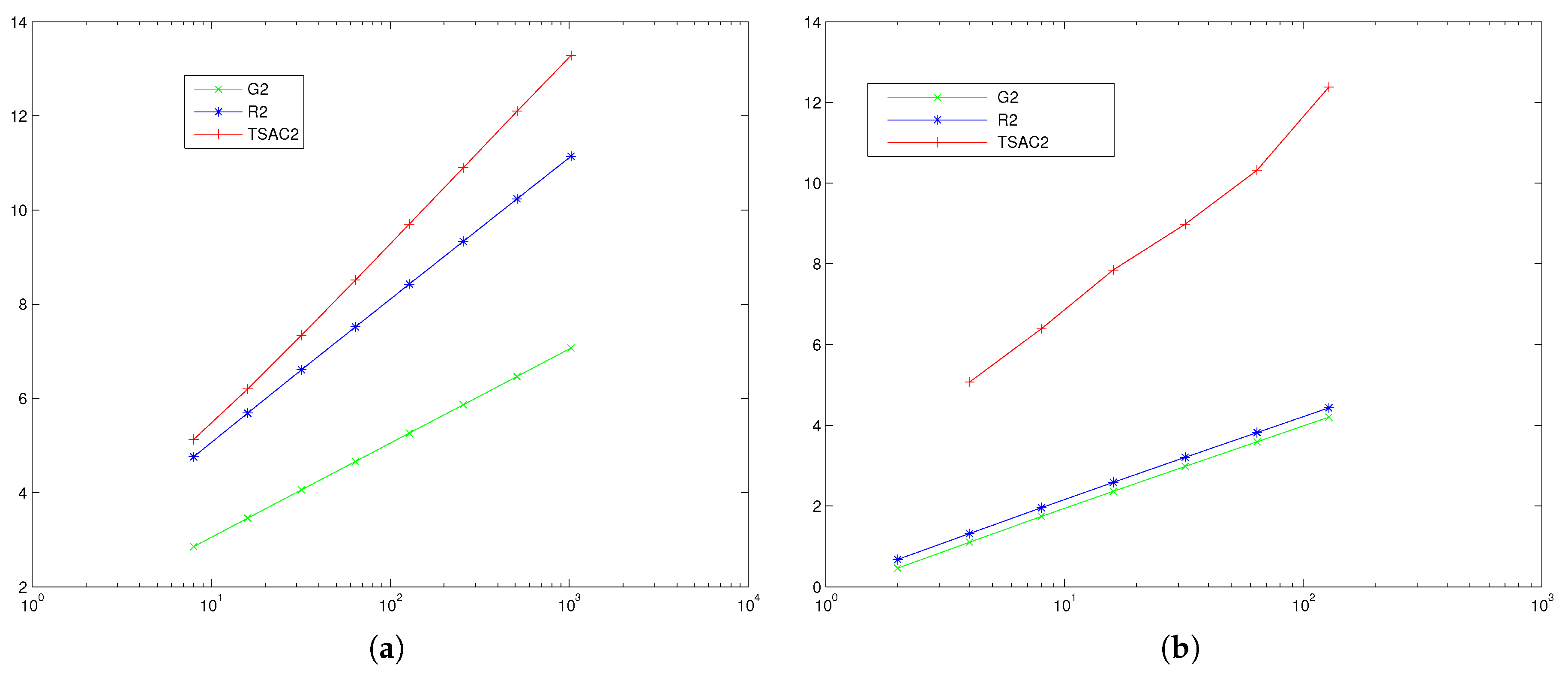
4.2. Numerical Results

We present some numerical results which confirm that, differently from one step collocation methods, the TSAC methods do not suffer form the order reduction in the integration of stiff systems, as we expect from the uniform order of convergence stated in Theorem 5. In order to illustrate this phenomenon, we show the results obtained on both a non stiff and a stiff equation:

• the non stiff VIE

  $$y(t)=2-cos(t)-{\displaystyle {\int }_0^t}sin(ty(\tau )-\tau )d\tau ,t\in [0,3],$$

  (37)

  with exact solution $y(t)\equiv 1$;
• the stiff VIE

  $$y(t)={\displaystyle {\int }_0^t}\left(\lambda \left(y(\tau )-sin(\tau )\right)+cos(\tau )\right)d\tau ,t\in [0,\frac{3}{4}\pi ],$$

  (38)

  with $\lambda =-{10}^4$ and exact solution $y(t)=\sin (t)$. This is a stiff problem because it is equivalent to the Prothero-Robinson problem for ODEs.

We compare TSAC methods with superconvergent one step collocation methods of [2,3], where m denotes the number of collocation points and p denotes the order of the method:

• G2: 1 point Gauss collocation, $c_2=1,m=2,p=2$;
• R2: 2 points Radau collocation, $m=2,p=3$;
• TSAC2: 2 points TSAC method, $m=2,p=4$.

The method TSAC2 is the two-stage TSAC method described in Example 1. The accuracy is defined by the number of correct significant digits $cd$ at the end point (the maximal absolute end point error is written as ${10}^{-cd}$). For each test we plot in Figure 1 the number of $cd$ versus the number of mesh points N. We observe as for non stiff Problem (37) the effective order of the all methods is coherent with the theoretical order, while for stiff Problem (38) the one step methods show order reduction as the effective order reduces to $p=2$.

Figure 1. Number of correct significant digits with respect to the number of mesh points. (a) Problem (37); (b) Problem (38).

5. One-Step Collocation Methods for VIDEs

We concentrate on VIDEs of type:

$$\begin{array}{c}\begin{array}{c}{y}^{\prime }(t)=g(t,y(t))+{\displaystyle {\int }_0^t}k(t,\tau ,y(\tau ))d\tau ,t\in I=[0,T],\hfill \\ y(0)=y_0,\hfill \end{array}\hfill \end{array}$$

(39)

where $g(t,y):I\times I{R}^d\to I{R}^d$, $k(t,s,y):S\times I{R}^d\to I{R}^d$, $S=\{(t,s)|0\le s\le t\le T\}$. For sake of completeness we report the theorem of existence and uniqueness of solution for (39) [3].

Theorem 6.

Let $g(t,y)$ and $k(t,s,y)$ be continuous functions and satisfy a uniform Lipschitz condition with respect to y. Then there exists a unique solution $y\in C^1([0,T])$ of the problem (39).

Let $I_h=\{t_n:0<t_0<t_1<\cdots <t_N=T\}$ be a partition of the time interval $[0,T]$ with constant stepsize $h=t_{n+1}-t_n$, $n=0,\dots ,N-1$. The integro-differential Equation (39) can be written as follows:

$$y^{\prime }(t)=g(t,y(t))+F_n(t,y(·))+{\mathsf{\Phi }}_n(t,y(·)),t\in [t_n,t_{n+1}],$$

where

$$\begin{array}{c}\hfill F_n(t,y(·))={\int }_0^{t_n}k(t,\tau ,y(\tau ))d\tau ,{\mathsf{\Phi }}_n(t,y(·))={\int }_{t_n}^{t}k(t,\tau ,y(\tau ))d\tau ,\end{array}$$

represent respectively the lag term and the increment function.

5.1. Exact One-Step Collocation Methods

Here we briefly expose the classical one-step collocation methods for VIDEs and their main properties [2,3].

A one-step collocation method approximates $y(t)$ by a piecewise polynomial $P(t)$, with $P(t)=P_n(t)$, $t\in [t_n,t_{n+1}]$, $n=0,\dots ,N-1$, where

$$P_n(t_n+sh)=y_n+h\sum _{j=1}^m{\beta }_j(s)U_{nj},s\in [0,1],$$

(40)

with $y_n=P_n(t_n)$, $U_{nj}=P_n^{\prime }(t_n+c_{j}h)$, ${\beta }_j(s)={\displaystyle {\int }_0^s}{L}_j(\tau )ds$, $L_j(\tau )$ being the j-th Lagrange fundamental polynomial with respect to the collocation parameters.

The m unknowns $U_{nj}$ are found by imposing that $P_n(t)$ satisfies (39) at the collocation points $t_{nj}:=t_n+c_{j}h,j=1,\dots ,m,n=0,\dots ,N-1$, where $0\le c_1<\dots <c_m\le 1$ are the collocation parameters.

The numerical approximation at the point $t_{n+1}$ is then given by $y_{n+1}=P_n(t_{n+1})$. The final form of an exact collocation method is

$$\left\{\begin{array}{cc}{U}_{ni}=\hfill & g(t_{ni},P_n(t_{ni}))+F_n(t_{ni},P(·))+{\mathsf{\Phi }}_n(t_{ni},P(·)),i=1,\dots ,m,\hfill \\ y_{n+1}=\hfill & y_n+h{\displaystyle \sum _{i=1}^m}{\beta }_j(1)U_{ni},\hfill \end{array}\right.$$

(41)

$n=0,\dots ,N$, where the lag term and the increment function can be written as

$$F_n(t_{ni},P(·))=h\sum _{\nu =0}^{n-1}{\int }_0^{1}k\left(t_{ni},t_{\nu }+\tau h,P_{\nu }(t_n+\tau h)\right)d\tau ,$$

(42)

$${\mathsf{\Phi }}_n(t_{ni},P(·))=h{\int }_0^{c_i}k\left(t_{ni},t_n+\tau h,P_n(t_n+\tau h)\right)d\tau .$$

(43)

The first equation in (41) requires, at each time step, the solution of an m-dimensional nonlinear system in the unknowns ${\{U_{ni}\}}_{i=1}^m$.

For every choice of the collocation parameters $c_1,\dots ,c_m$, the collocation polynomial $P(t)$ is continuous on $[0,T]$ and provides a uniform approximation of order $O(h^m)$. Moreover, if $c_1,\dots ,c_m$ are suitably chosen, the order of convergence at the mesh points increases (local superconvergence): is $2m-2$ for the Lobatto points, $2m-1$ for the Radau points and $2m$ for the Gauss ones [2,3].

5.2. Discretized One-Step Collocation Methods

In the general case, the integrals appearing in (42) and (43) cannot be exactly evaluated, so a further approximation is needed in order to fully discretize the method. Let us suppose to approximate these integrals by quadrature formulae of the type:

$${\tilde{F}}_n(t_{ni},P(·))=h\sum _{\nu =0}^{n-1}\sum _{l=1}^{{\mu }_1}{w}_{l}k(t_{ni},t_{\nu }+d_{l}h,P_{\nu }(t_{\nu }+d_{l}h)),$$

(44)

$${\tilde{\mathsf{\Phi }}}_n(t_{ni},P(·))=h\sum _{l=1}^{{\mu }_0}{w}_{il}k(t_{ni},t_n+d_{il}h,P_n(t_n+d_{il}h)).$$

(45)

These formulae are then used to define the discretized collocation methods as

$$\left\{\begin{array}{c}{\tilde{U}}_{ni}=g(t_{ni},{\tilde{P}}_n(t_{ni}))+{\tilde{F}}_n(t_{ni},\tilde{P}(·))+{\tilde{\mathsf{\Phi }}}_n(t_{ni},\tilde{P}(·))\hfill \\ {\tilde{y}}_{n+1}={\tilde{y}}_n+h{\displaystyle \sum _{i=1}^m}{\beta }_j(1){\tilde{U}}_{ni},\hfill \end{array}\right.$$

(46)

where the collocation polynomial is now of the form

$${\tilde{P}}_n(t_n+sh)=y_n+h\sum _{j=1}^m{\beta }_j(s){\tilde{U}}_{nj},s\in [0,1].$$

(47)

The discretized collocation methods are a special class of the Runge-Kutta extended methods and preserve the order of convergence and superconvergence of exact collocation methods, if the quadrature Formulae (44) and (45) are sufficiently accurate [3].

Some relevant stability results for one-step collocation methods are derived in [36,37].

6. Multistep Collocation for VIDEs

6.1. Exact Multistep Collocation

Recently, in order to obtain an higher order of convergence at the same computational effort, multistep collocation methods have been introduced: the solution $y(t)$ is approximated by a piecewise algebraic polynomial $P(t)$:

$$P(t_n+sh)=\sum _{k=0}^{r-1}{\phi }_k(s)y_{n-k}+h\sum _{j=1}^m{\psi }_j(s)U_{nj},s\in [0,1],$$

(48)

where again

$$U_{nj}:=P^{\prime }(t_{nj}),j=1,\dots ,m,$$

(49)

and the functions ${\phi }_k(s)$, ${\psi }_j(s)$ are polynomials of degree $m+r-1$ which are determined by imposing that the polynomial (48) satisfies (49) and the interpolation conditions:

$$P(t_{n-k})=y_{n-k},k=0,\dots ,r-1.$$

(50)

For any fixed set of collocation parameters $c_1,\dots ,c_m$, conditions (49) and (50) lead to the following non linear system of ${(r+m)}^2$ equations, where the ${(r+m)}^2$ unknowns are the coefficients of the polynomials ${\phi }_k(s)$ and ${\psi }_j(s)$:

$$\begin{array}{cc}{\phi }_l(-k)={\delta }_{lk},\hfill & {\phi }_l^{\prime }(c_j)=0,\hfill \\ {\psi }_i^{\prime }(c_j)={\delta }_{ij},\hfill & {\psi }_i(-k)=0,\hfill \end{array}$$

(51)

$l,k=0,\dots ,r-1,i,j=1,\dots ,m$.

Exact multistep collocation methods are obtained by imposing that the collocation polynomial (48) satisfies the VIDE at the collocation points $t_{ni}$, and by computing $y_{n+1}=P_n(t_{n+1})$:

$$\begin{array}{c}\hfill \left\{\begin{array}{cc}{U}_{ni}=\hfill & g(t_{ni},P(t_{ni}))+F_n(t_{ni},P(·))+{\mathsf{\Phi }}_n(t_{ni},P(·)),i=1,\dots ,m\hfill \\ y_{n+1}=\hfill & {\displaystyle \sum _{k=0}^{r-1}}{\phi }_k(1)y_{n-k}+h{\displaystyle \sum _{i=1}^m}{\psi }_j(1)U_{ni}.\hfill \end{array}\right.\end{array}$$

(52)

$n=r-1,\dots ,N$, where now the lag term and the increment function can be written as

$$\begin{array}{c}\hfill \begin{array}{c}{\displaystyle F_n(t_{ni},P(·))=h\sum _{\nu =0}^{n-1}{\int }_0^{1}k\left(t_{ni},t_{\nu }+\tau h,\sum _{k=0}^{r-1}{\phi }_k(\tau )y_{\nu -k}+h\sum _{j=1}^m{\psi }_j(\tau )U_{\nu j}\right)d\tau ,}\hfill \end{array}\end{array}$$

(53)

$$\begin{array}{c}\hfill \begin{array}{c}{\displaystyle {\mathsf{\Phi }}_n(t_{ni},P(·))=h{\int }_0^{c_i}k\left(t_{ni},t_n+\tau h,\sum _{k=0}^{r-1}{\phi }_k(\tau )y_{n-k}+h\sum _{j=1}^m{\psi }_j(\tau )U_{nj}\right)d\tau .}\hfill \end{array}\end{array}$$

(54)

We note that at each time step, the approximations $y_{n-k}$, $k=0,\dots ,r-1$ are already known, so only the unknowns ${\{U_{ni}\}}_{i=1}^m$ need to be computed, by solving the nonlinear system given by the first equation of (52).

Observe that we are able to give an approximate value $P(t)$ of the solution $y(t)$ at each point t of the integration interval, therefore we have a uniform approximation of the solution on $[0,T]$.

The classical one-step collocation methods described in the previous section can be seen as a particular case of multistep methods with $r=1$ and

$${\phi }_0(s)\equiv 1,{\psi }_j(s)={\int }_0^s{L}_j(\tau )d\tau ,$$

where $L_j(\tau )$ is the j-th Lagrange fundamental polynomial with respect to the collocation parameters. We observe that, at each time step, both one-step and multistep collocation methods require the solution of a non linear system of dimension m for the stages $U_{ni},i=1,\dots ,m$. The multistep methods only need in addition the computation of the starting values $y_1,\dots ,y_{r-1}$.

6.2. Discretized Multistep Collocation

As in the case of one-step collocation methods, it is evident that the exact multistep collocation methods (52) are not directly applicable for the implementation, since approximations of the integrals $F_n(t_{ni},P(·))$ and ${\mathsf{\Phi }}_n(t_{ni},P(·))$ are needed. With the aim of fully discretizing the multistep collocation methods we consider the following quadrature formulas

$$\begin{array}{c}\hfill \begin{array}{c}{\displaystyle {\int }_0^{c_i}\alpha (x)dx\approx Q_i(\alpha (·)):=\sum _{l=1}^{{\mu }_0}{w}_{il}\alpha (d_{il}),{\int }_0^1\alpha (x)dx\approx Q(\alpha (·)):=\sum _{l=1}^{{\mu }_1}{w}_l\alpha (d_l),}\hfill \end{array}\end{array}$$

(55)

where the weights and nodes are suitably chosen, as it will be illustrated later.

The discretized multistep collocation method for the problem (39) approximates the solution $y(t)$ with a piecewise polynomial $\tilde{P}(t)$, with

$$\tilde{P}(t_n+sh)=\sum _{k=0}^{r-1}{\phi }_k(s){\tilde{y}}_{n-k}+h\sum _{j=1}^m{\psi }_j(s){\tilde{U}}_{nj},s\in [0,1],$$

(56)

where the polynomials ${\{{\phi }_k(s)\}}_{k=0}^{r-1},{\{{\psi }_j(s)\}}_{j=1}^m$ are the same as in the exact collocation, and can be computed by solving the system (51).

We impose that at the collocation points $\tilde{P}(t)$ satisfies the VIDE (39), where the integrals appearing in both the lag term (53) and the increment function (54) are approximated by the quadrature formulae defined in (55), and we set ${\tilde{y}}_{n+1}=\tilde{P}(t_n+h)$. Thus the discretized multistep method is

$$\left\{\begin{array}{cc}{\tilde{U}}_{ni}=\hfill & {\displaystyle g(t_{ni},\tilde{P}(t_{ni}))+{\tilde{F}}_n(t_{ni},\tilde{P}(·))+{\tilde{\mathsf{\Phi }}}_n(t_{ni},\tilde{P}(·)),i=1,\dots ,m}\hfill \\ {\tilde{y}}_{n+1}=\hfill & {\displaystyle \sum _{k=0}^{r-1}{\phi }_k(1){\tilde{y}}_{n-k}+h\sum _{i=1}^m{\psi }_i(1){\tilde{U}}_{ni}.}\hfill \end{array}\right.$$

(57)

where ${\tilde{F}}_n(t_{ni},\tilde{P}(·))$ and ${\tilde{\mathsf{\Phi }}}_n(t_{ni},\tilde{P}(·))$ are of the form

$$\begin{array}{c}\hfill \begin{array}{c}{\displaystyle {\tilde{F}}_n(t_{ni},\tilde{P}(·))=h\sum _{\nu =0}^{n-1}\sum _{l=1}^{{\mu }_1}{w}_{l}k\left(t_{ni},t_{\nu }+d_{l}h,\sum _{k=0}^{r-1}{\phi }_k(d_l){\tilde{y}}_{\nu -k}+h\sum _{j=1}^m{\psi }_j(d_l){\tilde{U}}_{\nu j}\right)}\hfill \end{array}\\ \hfill \begin{array}{c}{\displaystyle {\tilde{\mathsf{\Phi }}}_n(t_{ni},\tilde{P}(·))=h\sum _{l=1}^{{\mu }_0}{w}_{il}k\left(t_{ni},t_n+d_{il}h,\sum _{k=0}^{r-1}{\phi }_k(d_{il}){\tilde{y}}_{n-k}+h\sum _{j=1}^m{\psi }_j(d_{il}){\tilde{U}}_{nj}\right).}\hfill \end{array}\end{array}$$

i.e., they are obtained by applying the quadrature Formula (55) to the integrals appearing in (53) and (54).

6.3. Convergence Analysis

The multivalue nature of the multistep methods imposes to analyze first the zero-stability of the methods. When $h\to 0$, second equation of (52) reduces to

$$y_{n+1}=\sum _{k=0}^{r-1}{\phi }_k(1)y_{n-k}.$$

Therefore, the method (48) and (52) is said to be zero-stable, if all of the roots of the polynomial

$$p(\lambda )={\lambda }^r-\sum _{k=0}^{r-1}{\phi }_k(1){\lambda }^{r-k-1}$$

(58)

have modulus less than or equal to unity, and those of modulus unity are simple.

On this basis, the following theorem studies the convergence of the method.

Theorem 7.

Consider the problem (39) with $d=1$. Let $p=m+r-1$ and assume that:

• $k\in C^p(S\times IR)$ and $g\in C^p([0,T]\times IR)$ and have bounded derivatives with respect to y;
• the method (48) and (52) is zero-stable;
• the starting error satisfies $\left|e(t)\right|=O(h^p)$, for any $t\in [t_0,t_{r-1}]$.

Then, the global error $e(t)=y(t)-P(t)$ of the exact MCM (48) and (52) satisfies

$$\underset{[0,T]}{max}\left|e(t)\right|\le C{h}^{m+r-1}.$$

(59)

By a suitable choice of the collocation parameters, it is possible to increase the order of convergence at the mesh points (local superconvergence), following the lines of multistep methods for ODEs (compare [21], Section 3).

Theorem 8.

Assume that hypotheses of Theorem 7 hold with $p=2m+r-1$ and that the collocation parameters satisfy these conditions

$$\sum _{k=-1}^{r-1}\frac{1}{c_i+k}+2\sum _{\begin{array}{c}j=1\\ j\ne i\end{array}}^m\frac{1}{c_i-c_j}=0,i=1,\dots ,m.$$

(60)

Then the order of the exact MCM (48) and (52) at the mesh points is p, i.e.,:

$$\underset{1\le n\le N}{max}\left|e(t_n)\right|=O(h^{2m+r-1}).$$

Similar convergence and superconvergence results hold also for the discretized MCM (56) and (57). We can summarize them in the following theorem.

Theorem 9.

Assume that hypotheses of Theorem 7 hold. If quadrature formulae Q and $Q_i$ defined in (55) have order $m+r$ and $m+r-1$ respectively, then the uniform order of the discretized method (56) and (57) is equal to $m+r-1$.

Moreover, if hypotheses of Theorem 8 are fulfilled, Q and $Q_i$ defined in (55) have order $2m+r$ and $2m+r-1$ respectively, then the order of the discretized method (56) and (57), at the mesh points, is $2m+r-1$.

We observe that, at the same cost of one-step collocation methods with m collocation parameters, multistep collocation methods have an higher computational cost. A further improvement of the efficiency could be obtained by exploiting parallel techniques, as done for example in [38,39,40].

An extensive analysis of the stability properties on basic test equations is contained in [14]. A possible future development may regard new multistep methods with some relaxing order conditions, which leave some parameters free to perform a numerical search for the methods with optimal stability properties, as done in [22,23,41,42,43] in the context of ODEs.

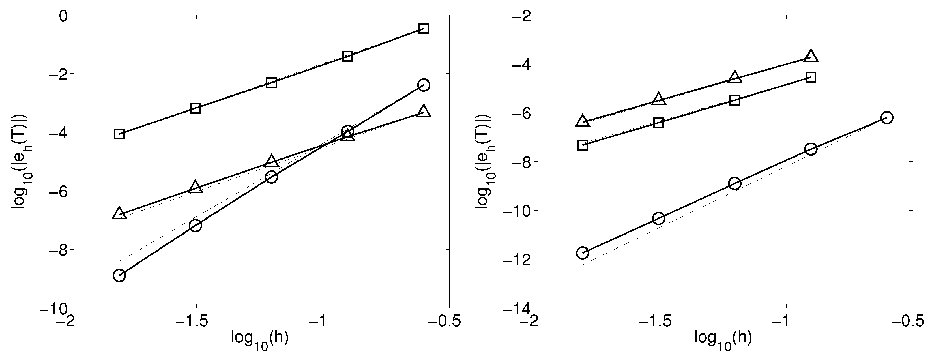
6.4. Numerical Results

Now we give a short numerical illustration of discretized MCMs (56) and (57), on the linear test equation

$$\begin{array}{c}\hfill \begin{array}{cc}{\displaystyle y^{\prime }(t)=g(t,y)-{\int }_0^t{t}^{2}exp(-st)y(s)ds,}\hfill & t\in [0,1],\hfill \\ y(0)=1,\hfill \end{array}\end{array}$$

(61)

with $g(t,y)$ such that $y(t)=exp(-t)$; and on the nonlinear problem

$$\begin{array}{c}\hfill \begin{array}{cc}{\displaystyle y^{\prime }(t)=g(t,y)-{\int }_0^{t}2tsin(s)exp(-y(s))ds,}\hfill & t\in [0,1],\hfill \\ y(0)=1,\hfill \end{array}\end{array}$$

(62)

with $g(t,y)$ such that $y(t)=cos(t)$.

We consider three methods

• TS3: superconvergent discretized two-step collocation method, with $r=2$ and $m=1$, with order $p=3$;
• TS3b: two-step discretized collocation method, with $r=2$ and $m=2$, $c_1=0.9$, $c_2=1$, with uniform order 3;
• TS5: superconvergent discretized two-step collocation method, with $r=2$ and $m=2$, with order $p=5$.

Method TS3b has an unbounded stability region, while TS3 and TS5 have a bounded stability region. The exact expression of the methods and their stability region can be found in [14]. To confirm the theoretical order of convergence, in Figure 2 the error (in logarithmic scale) produced by methods TS3, TS3b and TS5 when applied to problems (61) and (62), and the slopes corresponding to order 3 and 5. We see that the effective order is equal to the theoretical one.

Figure 2. Error of two-step methods TS3 (), TS3b () and TS5 (), and slopes of order 3 (dashed line) and of order 5 (dash-dot line), applied to problem (61) (left) and on problem (62) (right).

7. Conclusions

We have illustrated multistep collocation methods for VIEs and VIDEs and gave an overview of their convergence and superconvergence properties. This idea may be exploited to obtain high order methods for solving other types of equations as well. For example, recently two-step collocation methods have been proposed for fractional differential equations [44], and further developments may be achieved for other fractional models, as time fractional differential equations [45]. Further issues of this research will focus on oscillatory problems [46,47] and in particular on the application of multistep collocation methods to periodic integral equations [48,49]. Moreover, it seems reasonable to consider the possibility of employing collocation spaces based on functions other than polynomials, as in [50,51,52] and similarly as in the case of oscillatory problems [53], and merge into the numerical scheme as many known qualitative properties of the continuous problem as possible, in a structure-preserving perspective [54].

The literature on the numerical treatment of VIEs is quite rich and goes beyond the results considered in this review. Here we would like to mention some other results, at least. In [55] the modified Newton–Kantorovich method combined with collocation were applied non linear and nonlinear VIE with piecewise smooth kernels. Such VIE were introduced in [56] and asymptotic approximations to parametric families of solutions were constructed and the existence of continuous solutions was proved. The review of the numerical methods of optimal accuracy (spline-collocation technique) for multidimensional weakly singular VIEs is given in [57]. Some other interesting papers regard the distance between the approximate and exact solutions of various generalizations of the Volterra equations [58,59,60,61,62,63]. Lastly, we underline that in the practical applications of VIE based models it is extremely important to have the numerical method to be stable with respect to the measurement errors both in the source function and in the kernel. It is well known that the 1st kind of VIEs enjoy self-regularization property when the mesh step serves as the regularisation parameter. In addition, the Lavrentiev type regularisation is a good option [64,65]. These issues have been discussed in [66].

References

- Bonaccorsi, S.; Fantozzi, M. Volterra Integro-Differential Equations with Accretive Operators and Non-Autonomous Perturbations. J. Integral Equ. Appl. 2006, 18, 437–470. [Google Scholar] [CrossRef]
- Brunner, H. Collocation Methods for Volterra Integral and Related Functional Equations; Cambridge University Press: Cambridge, UK, 2004. [Google Scholar]
- Brunner, H.; van der Houwen, P.J. The Numerical Solution of Volterra Equations; CWI Monographs, 3; Elsevier Science Ltd.: Amsterdam, The Netherlands, 1986. [Google Scholar]
- Hoppensteadt, F.C.; Jackiewicz, Z.; Zubik-Kowal, B. Numerical solution of Volterra integral and integro-differential equations with rapidly vanishing convolution kernels. BIT Numer. Math. 2007, 47, 325–350. [Google Scholar] [CrossRef]
- Hrusa, W.J.; Renardy, M. A model problem in one-dimensional viscoelasticity with a singular kernel. In Volterra Integrodifferential Equations in Banach Spaces and Applications; Pitman Research Notes in Mathematics; da Prato, G., Iannelli, M., Eds.; Longman Scientific & Technical: Harlow, UK; Wiley: New York, NY, USA, 1989; Volume 190, pp. 221–230. [Google Scholar]
- Nohel, J.A.; Rogers, R.C.; Tzavaras, A.E. Hyperbolic conservation laws in viscoelasticity. In Volterra Integro Differential Equations in Banach Spaces and Applications; Da Prato, G., Iannelli, M., Eds.; Pitman Research Notes in Mathematics Series, 190; Longman Science Technology: Harlow, UK, 1989; pp. 320–338. [Google Scholar]
- Coleman, J.P.; Duxbury, S.C. Mixed collocation methods for y = f(x,y). J. Comput. Appl. Math. 2000, 126, 47–75. [Google Scholar] [CrossRef]
- Brunner, H.; Makroglou, A.; Miller, R.K. Mixed interpolation collocation methods for first and second order Volterra integro-differential equations with periodic solution. Appl. Numer. Math. 1997, 23, 381–402. [Google Scholar] [CrossRef]
- Braś, M.; Cardone, A.; Jackiewicz, Z.; Welfert, B. Order reduction phenomenon for general linear methods. J. Comput. Appl. Math. 2015, 290, 44–64. [Google Scholar] [CrossRef]
- Butcher, J.C. Numerical Methods for Ordinary Differential Equations, 2nd ed.; John Wiley & Sons: Chichester, UK, 2008. [Google Scholar]
- Hairer, E.; Wanner, G. Solving Ordinary Differential Equations. II. In Springer Series in Computational Mathematics; Springer: Berlin, Germany, 1991; Volume 14. [Google Scholar]
- D’Ambrosio, R.; Paternoster, B. Two-step modified collocation methods with structured coefficient matrices for ordinary differential equations. Appl. Numer. Math. 2012, 62, 1325–1334. [Google Scholar] [CrossRef]
- Capobianco, G.; Conte, D.; Paternoster, B. Construction and implementation of two-step continuous methods for Volterra Integral Equations. Appl. Numer. Math 2017, 119, 239–247. [Google Scholar] [CrossRef]
- Cardone, A.; Conte, D. Multistep collocation methods for Volterra integro-differential equations. Appl. Math. Comput. 2013, 221, 770–785. [Google Scholar] [CrossRef]
- Cardone, A.; Conte, D.; Paternoster, B. A family of multistep collocation methods for Volterra integro-differential equations. AIP Conf. Proc. 2009, 1168, 358–361. [Google Scholar] [CrossRef]
- Conte, D.; Paternoster, B. Multistep collocation methods for Volterra Integral Equations. Appl. Numer. Math. 2009, 59, 1721–1736. [Google Scholar] [CrossRef]
- Conte, D.; D’Ambrosio, R.; Paternoster, B. Two-step diagonally-implicit collocation-based methods for Volterra Integral Equations. Appl. Numer. Math. 2012, 62, 1312–1324. [Google Scholar] [CrossRef]
- Conte, D.; Jackiewicz, Z.; Paternoster, B. Two-step almost collocation methods for Volterra integral equations. Appl. Math. Comput. 2008, 204, 839–853. [Google Scholar] [CrossRef]
- Guillou, A.; Soulé, J.L. La résolution numérique des problèmes différentiels aux conditions initiales par des méthodes de collocation. Rev. Fr. Inform. Rech. Opér. 1969, 3, 17–44. [Google Scholar] [CrossRef]
- Lie, I. The stability function for multistep collocation methods. Numer. Math. 1990, 57, 779–787. [Google Scholar] [CrossRef]
- Lie, I.; Nørsett, S. Superconvergence for multistep collocation. Math. Comput. 1989, 52, 65–79. [Google Scholar] [CrossRef]
- Braś, M.; Cardone, A. Construction of Efficient General Linear Methods for Non-Stiff Differential Systems. Math. Model. Anal. 2012, 17, 171–189. [Google Scholar] [CrossRef]
- Braś, M.; Cardone, A.; D’Ambrosio, R. Implementation of explicit Nordsieck methods with inherent quadratic stability. Math. Model. Anal. 2013, 18, 289–307. [Google Scholar] [CrossRef]
- Jackiewicz, Z. General Linear Methods for Ordinary Differential Equations; John Wiley & Sons: Hoboken, NJ, USA, 2009. [Google Scholar]
- Darania, P. Superconvergence analysis of multistep collocation method for delay Volterra integral equations. Comput. Methods Differ. Equ. 2016, 4, 205–216. [Google Scholar]
- Darania, P.; Pishbin, S. High-order collocation methods for nonlinear delay integral equation. J. Comput. Appl. Math. 2017, 326, 284–295. [Google Scholar] [CrossRef]
- Fazeli, S.; Hojjati, G. Numerical solution of Volterra integro-differential equations by superimplicit multistep collocation methods. Numer. Algorithms 2015, 68, 741–768. [Google Scholar] [CrossRef]
- Fazeli, S.; Hojjati, G.; Shahmorad, S. Multistep Hermite collocation methods for solving Volterra integral equations. Numer. Algorithms 2012, 60, 27–50. [Google Scholar] [CrossRef]
- Fazeli, S.; Hojjati, G.; Shahmorad, S. Super implicit multistep collocation methods for nonlinear Volterra integral equations. Math. Comput. Model. 2012, 55, 590–607. [Google Scholar] [CrossRef]
- Fazeli, S.; Hojjati, G.; Shahmorad, S. Multistep collocation and iterated multistep collocation methods for solving two-dimensional Volterra integral equations. J. Mod. Methods Numer. Math. 2015, 6, 1–21. [Google Scholar] [CrossRef]
- Ma, J.; Xiang, S. A collocation boundary value method for linear Volterra integral equations. J. Sci. Comput. 2017, 71, 1–20. [Google Scholar] [CrossRef]
- Sheng, C.; Wang, Z.; Guo, B. A multistep Legendre-Gauss spectral collocation method for nonlinear Volterra integral equations. SIAM J. Numer. Anal. 2014, 52, 1953–1980. [Google Scholar] [CrossRef]
- Lopez-Fernandez, M.; Lubich, C.; Schadle, A. Adaptive, fast, and oblivious convolution in evolution equations with memory. SIAM J. Sci. Comput. 2008, 30, 1015–1037. [Google Scholar] [CrossRef]
- Lopez-Fernandez, M.; Lubich, C.; Schadle, A. Fast and oblivious convolution quadrature. SIAM J. Sci. Comput. 2006, 28, 421–438. [Google Scholar]
- Crisci, M.R.; Russo, E.; Vecchio, A. Stability results for one-step discretized collocation methods in the numerical treatment of Volterra integral equations. Math. Comput. 1992, 58, 119–134. [Google Scholar] [CrossRef]
- Crisci, M.R.; Russo, E.; Jackiewicz, Z.; Vecchio, A. Global stability of exact collocation methods for Volterra integro-differential equations. Atti Sem. Mat. Fis. Univ. Modena 1991, 39, 527–536. [Google Scholar]
- Crisci, M.R.; Russo, E.; Vecchio, A. Stability of Collocation Methods for Volterra Integro-Differential Equations. J. Integral Equ. Appl. 1992, 4, 491–507. [Google Scholar] [CrossRef]
- Cardone, A.; Messina, E.; Vecchio, A. An adaptive method for Volterra–Fredholm integral equations on the half line. J. Comput. Appl. Math. 2009, 228, 538–547. [Google Scholar] [CrossRef]
- Conte, D.; D’Ambrosio, R.; Paternoster, B. GPU acceleration of waveform relaxation methods for large differential systems. Numer. Algorithms 2016, 71, 293–310. [Google Scholar] [CrossRef]
- Conte, D.; Paternoster, B. Parallel methods for weakly singular Volterra Integral Equations on GPUs. Appl. Numer. Math. 2017, 114, 30–37. [Google Scholar] [CrossRef]
- Cardone, A.; Jackiewicz, Z.; Sandu, A.; Zhang, H. Extrapolated Implicit-Explicit Runge-Kutta Methods. Math. Model. Anal. 2014, 19, 18–43. [Google Scholar] [CrossRef]
- Conte, D.; D’Ambrosio, R.; Jackiewicz, Z.; Paternoster, B. A practical approach for the derivation of two-step Runge-Kutta methods. Math. Model. Anal. 2012, 17, 65–77. [Google Scholar] [CrossRef]
- Conte, D.; D’Ambrosio, R.; Jackiewicz, Z.; Paternoster, B. Numerical search for algebraically stable two-step continuous Runge-Kutta methods. J. Comput. Appl. Math. 2013, 239, 304–321. [Google Scholar] [CrossRef]
- Cardone, A.; Conte, D.; Paternoster, B. Two-step collocation methods for fractional differential equations. Discret. Contin. Dyn. Syst. Ser. B 2017, 22, 1–17. [Google Scholar] [CrossRef]
- Burrage, K.; Cardone, A.; D’Ambrosio, R.; Paternoster, B. Numerical solution of time fractional diffusion systems. Appl. Numer. Math. 2017, 116, 82–94. [Google Scholar] [CrossRef]
- Conte, D.; Paternoster, B. Modified Gauss-Laguerre exponential fitting based formulae. J. Sci. Comput. 2016, 69, 227–243. [Google Scholar] [CrossRef]
- Ixaru, L.G.; Paternoster, B. A Gauss quadrature rule for oscillatory integrands. Comput. Phys. Commun. 2001, 133, 177–188. [Google Scholar] [CrossRef]
- Cardone, A.; D’Ambrosio, R.; Paternoster, B. High order exponentially fitted methods for Volterra integral equations with periodic solution. Appl. Numer. Math. 2017, 114, 18–29. [Google Scholar] [CrossRef]
- Cardone, A.; Ixaru, L.G.; Paternoster, B.; Santomauro, G. Ef-Gaussian direct quadrature methods for Volterra integral equations with periodic solution. Math. Comput. Simul. 2015, 110, 125–143. [Google Scholar] [CrossRef]
- Cardone, A.; D’Ambrosio, R.; Paternoster, B. Exponentially fitted IMEX methods for advection—Diffusion problems. J. Comput. Appl. Math. 2017, 316, 100–108. [Google Scholar] [CrossRef]
- D’Ambrosio, R.; Moccaldi, M.; Paternoster, B. Adapted numerical methods for advection-reaction-diffusion problems generating periodic wavefronts. Comput. Math. Appl. 2017, 74, 1029–1042. [Google Scholar] [CrossRef]
- D’Ambrosio, R.; Paternoster, B. Numerical solution of reaction–diffusion systems of λ − ω type by trigonometrically fitted methods. J. Comput. Appl. Math. 2016, 294, 436–445. [Google Scholar] [CrossRef]
- D’Ambrosio, R.; De Martino, G.; Paternoster, B. General Nystrom methods in Nordsieck form: Error analysis. J. Comput. Appl. Math. 2016, 292, 694–702. [Google Scholar] [CrossRef]
- Butcher, J.; D’Ambrosio, R. Partitioned general linear methods for separable Hamiltonian problems. Appl. Numer. Math. 2017, 117, 69–86. [Google Scholar] [CrossRef]
- Muftahov, I.; Tynda, A.; Sidorov, D. Numeric solution of Volterra integral equations of the first kind with discontinuous kernels. J. Comput. Appl. Math. 2017, 313, 119–128. [Google Scholar] [CrossRef]
- Sidorov, D.N. On parametric families of solutions of Volterra integral equations of the first kind with piecewise smooth kernel. Differ. Equ. 2013, 49, 210–216. [Google Scholar] [CrossRef]
- Boykov, I.V.; Tynda, A.N. Numerical methods of optimal accuracy for weakly singular Volterra integral equations. Ann. Funct. Anal. 2015, 6, 114–133. [Google Scholar] [CrossRef]
- Castro, L.P.; Ramos, A. Hyers–Ulam–Rassias stability for a class of nonlinear Volterra integral equations. Banach J. Math. Anal. 2009, 3, 36–43. [Google Scholar] [CrossRef]
- Brzdek, J.; Eghbali, N. On approximate solutions of some delayed fractional differential equations. Appl. Math. Lett. 2016, 54, 31–35. [Google Scholar] [CrossRef]
- Bahyrycz, A.; Brzdek, J.; Lesniak, Z. On approximate solutions of the generalized Volterra integral equation. Nonlinear Anal. Real World Appl. 2014, 20, 59–66. [Google Scholar] [CrossRef]
- Gachpazan, M.; Baghani, O. Hyers-Ulam stability of nonlinear integral equation. Fixed Point Theory Appl. 2010, 2010, 927640. [Google Scholar] [CrossRef]
- Jung, S.M. A fixed point approach to the stability of a Volterra integral equation. Fixed Point Theory Appl. 2007, 2007, 057064. [Google Scholar] [CrossRef]
- Morales, J.R.; Rojas, E.M. Hyers–Ulam and Hyers–Ulam–Rassias stability of nonlinear integral equations with delay. Int. J. Nonlinear Anal. Appl. 2011, 2, 1–7. [Google Scholar]
- Kythy, P.K.; Puri, P. Computational Methods for Linear Integral Equations; Birkhauser: Boston, MA, USA, 2002. [Google Scholar]
- Muftahov, I.R.; Sidorov, D.N.; Sidorov, N.A. Lavrentiev regularization of integral equations of the first kind in the space of continuous functions. Izvestiya Irkutskogo Gosudarstvennogo Universiteta 2016, 15, 62–77. [Google Scholar]
- Muftahov, I.; Sidorov, D.; Zhukov, A.; Panasetsky, D.; Foley, A.; Li, Y.; Tynda, A. Application of Volterra Equations to Solve Unit Commitment Problem of Optimised Energy Storage and Generation. arXiv, 2016; arXiv:1608.05221. [Google Scholar]
© 2018 by the authors. Licensee MDPI, Basel, Switzerland. This article is an open access article distributed under the terms and conditions of the Creative Commons Attribution (CC BY) license (http://creativecommons.org/licenses/by/4.0/).