1. Introduction
The numerical solution of differential problems in the form
is needed in a variety of applications. In many relevant instances, the solution has important
geometric properties and the name
geometric integrator has been coined to denote a numerical method able to preserve them (see, e.g., the monographs [
1,
2,
3,
4]). Often, the geometric properties of the vector field are summarized by the presence of
constants of motion, namely functions of the state vector which are conserved along the solution trajectory of (
1). For this reason, in such a case one speaks about a
conservative problem. For sake of simplicity, let us assume, for a while, that there exists only one constant of motion, say
along the solution
of (
1). Hereafter, we shall assume that both
and
are suitably smooth (e.g., analytical). In order for the conservation property (
2) to hold, one requires that
Consequently, one obtains the equivalent condition
However, the conservation property (
2) can be equivalently restated through the vanishing of a line integral:
In fact, since
y satisfies (
1), one obtains that the integrand is given by
because of (
3). On the other hand, if one is interested in obtaining an approximation to
y, ruled by a discrete-time dynamics with time-step
h, one can look for any path
joining
to
, i.e.,
and such that
Definition 1. The path σ satisfying (5) and (6) defines aline integral method
providing an approximation to such that . Obviously, the process is then repeated on the interval
, starting from
, and so on. We observe that the path
now provides the vanishing of the line integral in (
6) without requiring the integrand be identically zero. This, in turn, allows much more freedom during the derivation of such methods. In addition to this, it is important to observe that one cannot, in general, directly impose the vanishing of the integral in (
6) since, in most cases, the integrand function does not admit a closed form antiderivative. Consequently, in order to obtain a
ready to use numerical method, the use of a suitable quadrature rule is mandatory.
Since we shall deal with
polynomial paths , it is natural to look for an interpolatory quadrature rule defined by the abscissae and weights
,
. In order to maximize the order of the quadrature, i.e.,
, we place the abscissae at the zeros of the
kth shifted and scaled Legendre polynomial
(i.e.,
,
). Such polynomials provide an orthonormal basis for functions in
:
with
denoting the Kronecker delta. Consequently, (
6) becomes
Definition 2. The path σ satisfying (5) and (8) defines adiscrete line integral method
providing an approximation to such that , within the accuracy of the quadrature rule. As is clear, if
C is such that the quadrature in (
8) is exact, then the method reduces to the line integral method satisfying (
5) and (
6), exactly conserving the invariant. In the next sections we shall make the above statements more precise and operative.
Line integral methods were at first studied to derive energy-conserving methods for Hamiltonian problems: a coarse idea of the methods can be found in [
5,
6]; the first instances of such methods were then studied in [
7,
8,
9]; later on, the approach has been refined in [
10,
11,
12,
13] and developed in [
14,
15,
16,
17,
18]. Further generalizations, along several directions, have been considered in [
19,
20,
21,
22,
23,
24,
25,
26,
27,
28]: in particular, in [
19] Hamiltonian boundary value problems have been considered, which are not covered in this review. The main reference on line integral methods is given by the monograph [
1].
With these premises, the paper is organized as follows: in
Section 2 we shall deal with the numerical solution of Hamiltonian problems; Poisson problems are then considered in
Section 3; constrained Hamiltonian problems are studied in
Section 4; Hamiltonian partial differential equations (PDEs) are considered in
Section 5; highly oscillatory problems are briefly discussed in
Section 6; at last,
Section 7 contains some concluding remarks.
2. Hamiltonian Problems
A canonical Hamiltonian problem is in the form
with
H the
Hamiltonian function and, in general,
hereafter denoting the identity matrix of dimension
r. Because of the skew-symmetry of
J, one readily verifies that
H is a constant of motion for (
9):
For isolated mechanical systems,
H has the physical meaning of the total energy, so that it is often referred to as the
energy. When solving (
9) numerically, it is quite clear that this conservation property becomes paramount to get a correct simulation of the underlying phenomenon. The first successful approach in the numerical solution of Hamiltonian problems has been the use of
symplectic integrators. The characterization of a symplectic Runge-Kutta method
is based on the following algebraic property of its Butcher tableau [
29,
30] (see also [
31])
which is tantamount to the conservation of any quadratic invariant of the continuous problem.
Under appropriate assumptions, symplectic integrators provide a bounded Hamiltonian error over long time intervals [
2], whereas generic numerical methods usually exhibit a drift in the numerical Hamiltonian. Alternatively, one can look for
energy conserving methods (see, e.g., [
32,
33,
34,
35,
36,
37,
38,
39]). We here sketch the
line integral solution to the problem. According to (
5) and (
6) with
, let us set
where the coefficients
are at the moment unknown. Integrating term by term, and imposing the initial condition, yields the following polynomial of degree
s:
By defining the approximation to
as
where we have taken into account the orthonormality conditions (
7), so that
, one then obtains that the conditions (
5) are fulfilled. In order to fulfil also (
6) with
, one then requires, by taking into account (
11)
This latter equation is evidently satisfied, due to the skew-symmetry of J, by setting
Consequently, (
12) becomes
which, according to ([
12], Definition 1), is the
master functional equation defining
. Consequently, the conservation of the Hamiltonian is assured. Next, we discuss the order of accuracy of the obtained approximation, namely the difference
: this will be done in the next section, by using the approach defined in [
18].
2.1. Local Fourier Expansion
By introducing the notation
one has that (
9) can be written, on the interval
, as
with
defined according to (
16), by formally replacing
with
y. Similarly,
with the polynomial
in (
15) satisfying, by virtue of (
11) and (
14), the differential equation:
The following result can be proved (see [
18], Lemma 1).
Lemma 1. Let , with V a vector space, admit a Taylor expansion at 0. Then, for all Moreover, let us denote by
the solution of the ODE-IVPs
and by
the fundamental matrix solution of the variational problem associated to it. We recall that
We are now in the position to prove the result concerning the accuracy of the approximation (
13).
Theorem 1. (in other words, the polynomial σ defines an approximation procedure of order 2s).
Proof. One has, by virtue of (
5), (
16)–(
19), Lemma 1, and (
20):
☐
2.2. Hamiltonian Boundary Value Methods
Quoting Dahlquist and Björk [
40], p. 521,
as is well known, even many relatively simple integrals cannot be expressed in finite terms of elementary functions, and thus must be evaluated by numerical methods. In our framework, this obvious statement means that, in order to obtain a numerical method from (
15), we need to approximate the integrals appearing in that formula by means of a suitable quadrature procedure. In particular, as anticipated above, we shall use the Gauss-Legendre quadrature of order
, whose abscissae and weights will be denoted by
(i.e.,
,
). Hereafter, we shall obviously assume
. In so doing, in place of (
15), one obtains a (possibly different) polynomial,
where (see (
16)):
with
the quadrature error. Considering that the quadrature is exact for polynomial integrands of degree
, one has:
As a consequence,
if
H is a polynomial of degree
. In such a case,
, i.e., the energy is exactly conserved. Differently, one has, by virtue of (
22) and Lemma 1:
The result of Theorem 1 continues to hold for
u. In fact, by using arguments similar to those used in the proof of that theorem, one has, by taking into account (
22) and that
:
Definition 3. The polynomial u defined at (21) defines a Hamiltonian Boundary Value Method (HBVM) with parameters k and s, in short HBVM. Actually, by observing that in (
21) only the values of
u at the abscissae are needed, one obtains, by setting
, and rearranging the terms:
with the new approximation given by
Consequently, we are speaking about the
k-stage Runge-Kutta method with Butcher tableau given by:
with
and
The next result summarizes the properties of HBVMs sketched above, where we also take into account that the abscissae are symmetrically distributed in the interval [0, 1] (we refer to [
1,
18] for full details).
Theorem 2. For all , a HBVM method:
is symmetric and ;
when it becomes the s-stage Gauss collocation Runge-Kutta method;
it is energy conserving when the Hamiltonian H is a polynomial of degree not larger than ;
conversely, one has .
We conclude this section by showing that, for HBVM, whichever is the value considered, the discrete problem to be solved has dimension s, independently of k. This fact is of paramount importance, in view of the use of relatively large values of k, which are needed, in order to gain a (at least practical) energy conservation. In fact, even for non polynomial Hamiltonians, one obtains a practical energy conservation, once the Hamiltonian error falls, by choosing k large enough, within the round-off error level.
By taking into account the stage Equation (
24), and considering that
, one has that the stage vector can be written as
where
and
is the block vector (of dimension
s) with the coefficients (
22) of the polynomial
u in (
21). By combining (
29) and (
31), one then obtains the discrete problem, equivalent to (
24),
having (block) dimension
s,
independently of k. Once this has been solved, one verifies that the new approximation (
25) turns out to be given by (compare also with (
13)):
Next section will concern the efficient numerical solution of the discrete problem
generated by the application of a HBVM
method. In fact, a straightforward fixed-point iteration,
may impose severe stepsize limitations. On the other hand, the application of the simplified Newton iteration for solving (
34) reads, by considering that (see (
27) and (
28))
and setting
the Jacobian of
f evaluated at
:
This latter iteration, in turn, needs to factor a matrix whose size is s times larger than that of the continuous problem. This can represent an issue, when large-size problems are to be solved and/or large values of s are considered.
2.3. Blended Implementation of HBVMs
We here sketch the main facts concerning the so called
blended implementation of HBVMs, a Newton-like iteration alternative to (
36), which only requires to factor a matrix having the same size as that of the continuous problem, thus resulting into a much more efficient implementation of the methods [
1,
16]. This technique derives from the definition of
blended implicit methods, which have been at first considered in [
41,
42], and then developed in [
43,
44,
45]. Suitable blended implicit methods have been implemented in the Fortran codes BIM [
46], solving stiff ODE-IVPs, and BIMD [
47], also solving linearly implicit DAEs up to index 3. The latter code is also available on the
Test Set for IVP Solvers [
48] (see also [
49]), and turns out to be among the most reliable and efficient codes currently available for solving stiff ODE-IVPs and linearly implicit DAEs. It is worth mentioning that, more recently, the blended implementation of RKN-type methods has been also considered [
50].
Let us then consider the iteration (
36), which requires the solution of linear systems in the form
By observing that matrix
defined at (
35) is nonsingular, we can consider the
equivalent linear system
where
is a positive parameter to be determined. For this purpose, let
be the Jordan canonical form of
. For simplicity, we shall assume that
is diagonal, and let
be any of its diagonal entries. Consequently, the two linear systems (
37) and (
38), projected in the invariant subspace corresponding to that entry, respectively become
again being equivalent to each other (i.e., having the same solution
). We observe that the coefficient matrix of the former system is
, when
, whereas that of the latter one is
, when
. Consequently, one would like to solve the former system, when
, and the latter one, when
. This can be done automatically by considering a
weighting function such that
then considering the
blending of the two equivalent systems (
39) with weights
and
, respectively:
In particular, (
40) can be accomplished by choosing
Consequently, one obtains that
As a result, one can consider the following splitting for solving the problem:
The choice of the scalar parameter
is then made in order to optimize the convergence properties of the corresponding iteration. According to the analysis in [
42], we consider
where, as is usual,
denotes the spectrum of matrix
. A few values of
are listed in
Table 1.
Coming back to the original iteration (
36), one has that the weighting function (
42) now becomes
which requires to factor only the matrix
having the same size as that of the continuous problem, thus obtaining the following
blended iteration for HBVMs:
It is worth mentioning that:
in the special case of separable Hamiltonian problems, the blended implementation of the methods can be made even more efficient, since the discrete problem can be cast in terms of the generalized coordinates only (see [
16] or ([
1], Chapter 4));
the coding of the blended iteration becomes very high-performance by considering a matrix formulation of (
45) (see, e.g., ([
1], Chapter 4.2.2) or [
51]). As matter of fact, it has been actually implemented in the Matlab code
hbvm, which is freely available on the internet at the url [
52].
In order to give evidence of the usefulness of energy conservation, let us consider the solution of the well-known pendulum problem, with Hamiltonian
When considering the trajectory starting at [
1,
53]
one obtains a periodic solution of period
. In
Table 2 we list the obtained results when solving the problem over 10 periods, by using a stepsize
, with HBVM(6,3) and HBVM(3,3) (i.e., the symplectic 3-stage Gauss collocation method), for increasing values of
n. As one may see, even though both methods are 6th order accurate, nevertheless, HBVM(6,3) becomes (practically) energy-conserving as soon as
, whereas HBVM(3,3) does not. One clearly sees that, for the problem at hand, the energy-conserving method is pretty more accurate than the non conserving one.
2.4. Energy and QUadratic Invariants Preserving (EQUIP) Methods
According to Theorem 2, when
, HBVM
reduces to the
s-stage Gauss method. For such a method, one has, with reference to (
26)–(
28) and (
35) with
,
so that the Butcher matrix in (
26) becomes the
W-transformation [
54] of the
s-stage Gauss method, i.e., the Butcher matrix is
. Moreover, since
, the method is easily verified to be symplectic, because of (
10). In fact, by setting in general
the
ith unit vector, and with reference to the vector
defined in (
30) with
, one has:
We would arrive at the very same conclusion if we replace by
In particular, if the parameter
is small enough, matrix
will act as a perturbation of the underlying Gauss formula and the question is whether it is possible to choose
, at each integration step, such that the resulting integrator may be energy conserving. In order for
, we need to assume, hereafter,
. In particular, by choosing
it is possible to show [
26] that the scalar parameter
can be chosen, at each integration step, such that, when solving the Hamiltonian problem (
9) with a sufficiently small stepsize
h:
This fact is theoretically intriguing, since this means that we have a kind of state-dependent Runge-Kutta method, defined by the Butcher tableau
which is energy conserving and is defined, at each integration step, by a symplectic map, given by a small perturbation of that of the underlying
s-stage Gauss method. Consequently, EQUIP methods do not infringe the well-known result about the nonexistence of energy conserving symplectic numerical methods [
55,
56]. Since the symplecticity condition (
10) is equivalent to the conservation of all quadratic invariants of the problem, these methods have been named
Energy and QUadratic Invariants Preserving (
EQUIP) methods [
26,
57]. It would be interesting to study the extent to which the solutions generated by an EQUIP method inherit the good long time behavior of the associated Gauss integrator with reference to the nearly conservation property of further non-quadratic first integrals. This investigation would likely involve a backward error analysis approach, similar to that done in [
2], and up to now remains an open question.
For a thorough analysis of such methods we refer to [
26,
53]. In the next section, we sketch their line-integral implementation when solving Poisson problems, a wider class than that of Hamiltonian problems.
3. Poisson Problems
Poisson problems are in the form
When
as defined in (
9), then one retrieves canonical Hamiltonian problems. As in that case, since
is skew-symmetric, then
H, still referred to as the
Hamiltonian, is conserved:
Moreover, any scalar function
such that
is also conserved, since:
C is called a
Casimir function for (
50). Consequently, all possible Casimirs and the Hamiltonian
H are conserved quantities for (
50). In the sequel, we show that EQUIP methods can be conveniently used for solving such problems. As before, the scalar parameter
in (
49) is selected in such a way that the Hamiltonian
H is conserved. Moreover, since the Butcher matrix in (
49) satisfies (
10), then all quadratic Casimirs turn out to be conserved as well. The conservation of all quadratic invariants, in turn, is an important property as it has been observed in [
58].
Let us then sketch the choice of the parameter
to gain energy conservation (we refer to [
53] for full details). By setting
one has that the Butcher matrix in (
49) can be written as
Consequently, by denoting
, and setting
,
, the stages of the method, one obtains that the polynomial
is given by
with the (block) vectors
formally defined as in (
22) with
. In vector form, one has then (compare with (
31)):
We observe that, from (
51), one also obtains:
Nevertheless, the new approximation, still given by
now differs from
Consequently, in order to define a path joining
to
, to be used for imposing energy-conservation by zeroing a corresponding line-integral, we can consider the polynomial path made up by
u plus
As a result, by considering that
,
,
, we shall choose
such that (see (
51)–(
56)):
In more details, by defining the vectors
and resorting to the usual line integral argument, it is possible to prove the following result ([
53], Theorem 2).
Theorem 3. (57) holds true, provided that As in the case of HBVMs, however, we shall obtain a practical numerical method only provided that the integrals in (
58) are suitably approximated by means of a quadrature which, as usual, we shall choose as the Gauss-Legendre formula of order
. In so doing, one obtains an
EQUIP method. The following result can be proved ([
53], Theorem 8).
Theorem 4. Under suitable regularity assumptions on both and , one has that for all , the EQUIP method has order , conserves all quadratic invariants and, moreover, We observe that, for EQUIP
, even a not exact conservation of the energy may result in a much better error growth, as the next example shows. We consider the Lotka-Volterra problem [
53], which is in the form (
50) with
By choosing the following parameters and initial values,
one obtains a periodic solution of period
. If we solve the problems (
60) and (
61) with the EQUIP(6,3) and the 3-stage Gauss methods with stepsize
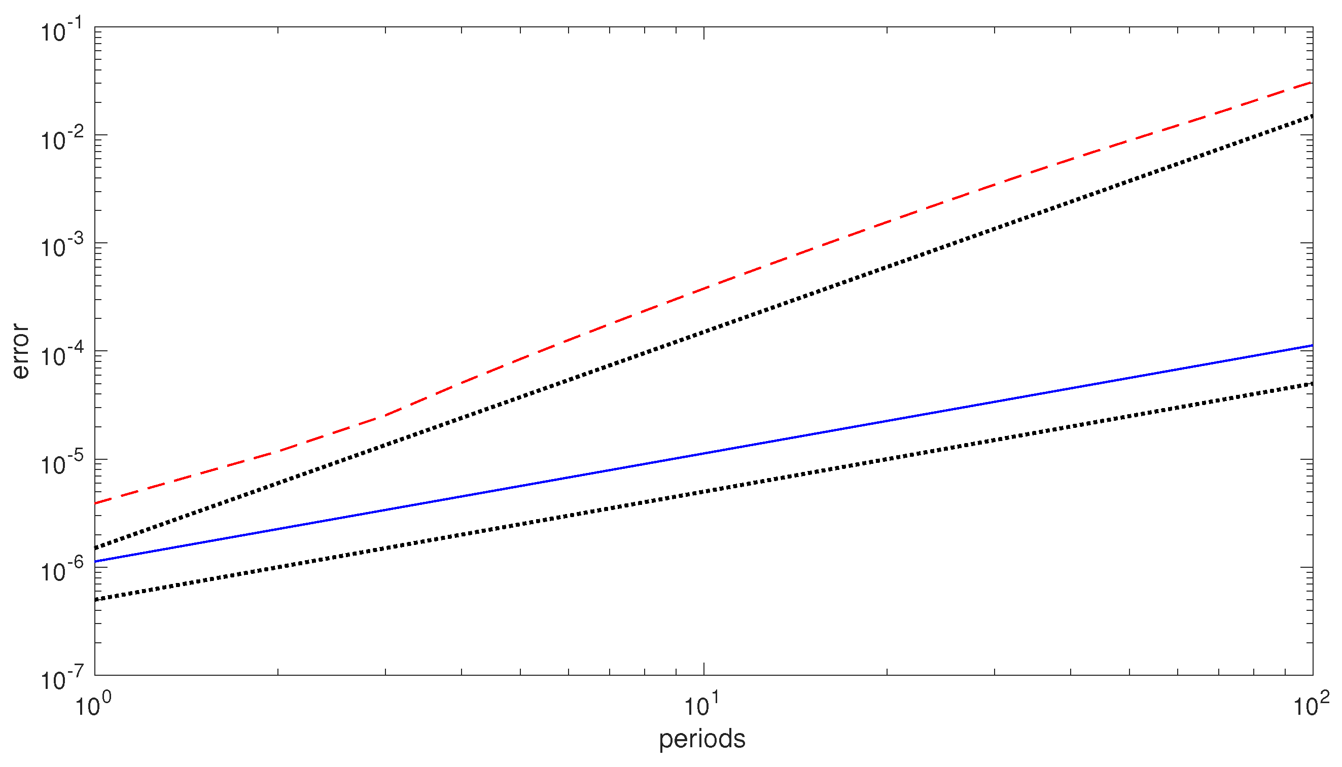
over 100 periods, we obtain the error growths, in the numerical solution, depicted in
Figure 1. As one may see, the EQUIP(6,3) method (which only approximately conserves the Hamiltonian), exhibits a
linear error growth; on the contrary, the 3-stage Gauss method (which exhibits a drift in the numerical Hamiltonian) has a
quadratic error growth. Consequently, there is numerical evidence that EQUIP methods can be conveniently used for numerically solving Poisson problems (a further example can be found in [
53]).
4. Constrained Hamiltonian Problems
In this section, we report about some recent achievements concerning the line integral solution of constrained Hamiltonian problems with holonomic contraints [
23]. This research is at a very early stage and, therefore, it is foreseeable that new results will follow in the future.
To begin with, let us consider the separable problem defined by the Hamiltonian
with
M a symmetric and positive definite matrix, subject to the
holonomic constraints
We shall assume that the points are regular for the constraints, so that
has full column rank and, therefore, the
matrix
is nonsingular. By introducing the vector of the Lagrange multipliers
, problems (
62) and (
63) can be equivalently cast in Hamiltonian form by defining the augmented Hamiltonian
thus obtaining the equivalent constrained problem:
subject to the initial conditions
We observe that the first requirement (
) obviously derives from the given constraints. The second, in turn, derives from
which has to be satisfied by the solution of (
65). These latter constraints are sometimes referred to as the
hidden constraints. A formal expression of the vector of the Lagrange multipliers can be obtained by further differentiating the previous expression, thus giving
which is well defined, because of the assumption that
is nonsingular. Consequently,
where the notation
means that the vector
is a function of
q and
p. It is easily seen that both the two Hamiltonians (
62) and (
64) are conserved along the solution of the problems (
65) and (
66), and assume the same value. For numerically solving the problem, we shall consider a discrete mesh with time-step
h, i.e.,
,
, looking for approximations
such that, starting from
, one arrives at
by choosing
in order for:
Consequently, the new approximation conserves the Hamiltonan and exactly satisfies the constraints, but only approximately the hidden contraints. In particular, we shall consider a piecewise constant approximation of the vector of the Lagrange multipliers
, i.e.,
is assumed to be constant on the interval
. In other words, we consider the sequence of problems (compare with (
65)), for
:
where the constant vector
is chosen in order to satisfy the constraints at
. That is, such that the new approximations, defined as
satisfy (
68). The reason for choosing
as a constant vector stems from the following result, which concerns the augmented Hamiltonian (
64).
Theorem 5. For all , the solution of (69) and (70) satisfies . Proof. In fact, denoting by
the gradient of
with respect to the
q variables, and similarly for
, the usual line integral argument provides:
☐
Consequently, one obtains that
i.e., energy conservation is equivalent to satisfy the constraints.
In order to fulfil the constraints, we shall again resort to a line integral argument. For this purpose, we need to define the Fourier coefficients (along the Legendre basis (
7)) of the functions appearing at the right-hand sides in (
69):
so that, in particular,
We also need the following result.
Lemma 2. With reference to matrix defined in (35), one has, for all : Proof. See, e.g., ([
23], Lemma 2). ☐
We are now in the position of deriving a formal expression for the constant approximation to the vector of the Lagrange multipliers through the usual line integral approach:
Because of Lemma 2, one then obtains that (see (
35)),
The following result can be proved [
23].
Theorem 6. The Equation (73) is consistent with (67) and is well defined for all sufficiently small . The sequence generated by (69)–(73) satisfies, for all : Moreover, in the case where , for all , then , , .
At this point, in order to obtain a numerical method, the following two steps need to be done:
truncate the infinite series in (
72) to finite sums, say up to
. In so doing, the expression of
changes accordingly, since in (
73) the infinite sums will consequently arrive up to
;
approximate the integrals in (
71), for
. As usual, we shall consider a Gauss-Legendre formula of order
, with
, thus obtaining corresponding approximations which we denote, for
,
In so doing, it can be seen that one retrieves the usual HBVM
method defined in
Section 2, applied for solving (
69), coupled with the following equation for
, representing the approximation of (
73):
The following result can be proved [
23].
Theorem 7. For all sufficiently small stepsizes h, the HBVM method coupled with (74), used for solving (65) and (66) over a finite interval, is well defined and symmetric. It provides a sequence of approximations such that (see (67)): Moreover, in the case where , for all , then It is worth mentioning that, even in the case where the vector of the Lagrange multipliers is not constant, so that all HBVM are second-order accurate for all , the choice generally provides a much smaller solution error.
We refer to [
23] for a number of examples of application of HBVMs to constrained Hamiltonian problems. We here only provide the application of HBVM(4,4) (together with (
74) with
) for solving the so called
conical pendulum problem. In more details, let us have a pendulum of unit mass connected to a fixed point (the origin) by a massless rod of unit length. The initial conditions are such that the motion is periodic of period
T and takes place in the horizontal plane
. Normalizing the acceleration of gravity, the augmented Hamiltonian is given by
where
and
is the
ith unit vector. Choosing
,
, results in
Since the augmented Hamiltonian
is quadratic and
is constant, any HBVM
method, coupled with (
74), is energy and constraint conserving, and of order
. If we apply the HBVM(4,4) method for solving the problem over 10 periods by using the stepsize
,
, it turns out the
,
,
, and
within the round-off error level, for all
. On the other hand, the corresponding solution errors, after 10 periods, turn out to be given by 4.9944 × 10
, 1.9676 × 10
, 7.3944 × 10
, thus confirming the order 8 of convergence of the resulting method.
5. Hamiltonian PDEs
Quoting [
4], p. 187,
the numerical solution of time dependent PDEs may often be conceived as consisting of two parts. First the spatial derivatives are discretized by finite differences, finite elements, spectral methods, etc. to obtain a system of ODEs, with t as the independent variable. Then this system of ODEs is integrated numerically. If the PDEs are of Hamiltonian type, one may insist that both stages preserve the Hamiltonian structure. Thus the space discretization should be carried out in such a way that the resulting system of ODEs is Hamiltonian (for a suitable Poisson bracket). This approach has been systematically used for solving a number of Hamiltonian PDEs by using HBVMs [
1,
20,
22,
59,
60] and this research is still under development. We here sketch te main facts for the simplest possible example, provided by the semilinear wave equation,
with
the derivative of
f, coupled with the initial conditions
and periodic boundary conditions. We shall assume that
f,
,
are regular enough (the last two functions, as periodic functions). By setting (hereafter, when not necessary, we shall avoid the arguments of the functions)
so that
,
, the problem can be cast into Hamiltonian form as
i.e.,
where
is the vector of the functional derivatives [
2,
3,
22] of the
Hamiltonian functionalBecause of the periodic boundary conditions, this latter functional turns out to be conserved. In fact, by considering that
one obtains:
because of the periodicity in space. Consequently,
Moreover, since
is periodic for
, we can expand it in space along the following slight variant of the Fourier basis,
so that, for all allowed
:
In so doing, for suitable time dependent coefficients
, one obtains the expansion:
having introduced the infinite vectors
By considering that
the identity operator, and introducing the infinite matrix (see (
77))
so that
and
, one then obtains that (
79) can be rewritten as the infinite system of ODEs:
subject to the initial conditions (see (
76))
The following result is readily established.
Theorem 8. Problem (87) is Hamiltonian, with Hamiltonian This latter is equivalent to the Hamiltonian functional (80), via the expansion (83). Proof. The first part of the proof is straightforward. Concerning the second part, one has, by virtue of (
85):
Similarly, by considering that
, one obtains:
☐
In order to obtain a computational procedure, one needs to truncate the infinite series in (
83) to a finite sum, i.e.,
Clearly, such an approximation no longer satisfies the wave Equation (
79). Nevertheless, in the spirit of Fourier–Galerkin methods [
61], by requiring that the residual be orthogonal to the functional subspace
containing the approximation
for all times
, one obtains a finite dimensional ODE system, formally still given by (
87) and (
88), upon replacing the involved infinite vectors and matrices, previously defined in (
84) and (
86), with the following finite dimensional ones (of dimension
):
Moreover, the result of Theorem 8 continues formally to hold for the finite dimensional problem, with the sole exception that now the Hamiltonian (
89) only yields an approximation to the continuous functional (
80). Nevertheless, it is well known that, under suitable regularity assumptions on
f and the initial data, this truncated version converges exponentially to the original functional (
80), as
(this phenomenon is usually referred to as
spectral accuracy). Since problem (
87) is Hamiltonian, one can use HBVM
methods for solving it. It is worth mentioning that, in so doing, the blended implementation of the methods can be made extremely efficient, by considering that:
Consequently, the Jacobian matrix of (
87) can be approximated by the linear part alone, i.e., as
This implies that matrix
involved in the definition of
in (
44) becomes (all the involved matrices are diagonal and have dimension
):
where
is the parameter defined in (
43), and
h is the used time-step. As a result,
:
is constant for all time steps, so that it has to be computed only once;
it has a block diagonal structure (and, in particular, is positive definite).
The above features make the resulting blended iteration (
45) inexpensive, thus allowing the use of large values of
N and large time-steps
h. As an example, let us solve the
sine-Gordon equation [
22],
with
, whose solution is, by considering the value
,
In such a case, the value
in (
90) and (
91) is sufficient to obtain an error in the spatial semi-discretization comparable with the round-off error level. Then, we solve in time the semi-discrete problem (
87), of dimension
, by using the HBVM
methods. In
Table 3 we list the obtained maximum errors in the computed solution, by using a time-step
, along with the corresponding Hamiltonian errors and execution times, for various choices of
(in particular, for
,
, we have the
s-stage Gauss collocation methods, which are symplectic but not energy conserving) (all numerical tests have been performed on a laptop with a 2.2 GHz dual core i7 processor, 8 GB of memory, and running Matlab R2017b). From the listed results, one sees that HBVM
methods become energy-conserving for
and the error decreases until the round-off error level, for
, with a computational time 10 times larger than that of the implicit mid-point rule (obtained for
) which, however, has a solution error
times larger.
6. Highly Oscillatory Problems
The Hamiltonian system of ODEs (
87) is a particular instance of problems in the form
where, without loss of generality,
A is a symmetric and positive definite matrix and
f is a scalar function such that
in a neighbourhood of the solution. Moreover, hereafter we consider the 2-norm, so that
equals the largest eigenvalue of
A (in general, any convenient upper bound would suffice). The problem is Hamiltonian, with Hamiltonian
Problems in the form (
94) satisfying (
95) are named
(multi-frequency) highly oscillatory problems, since they are ruled by the linear part, possessing large (possibly different) complex conjugate eigenvalues. Such problems have been investigated since many years, starting from the seminal papers [
62,
63], and we refer to the monograph [
64] for more recent findings. A common feature of the methods proposed so far, however, is that of requiring the use of time-steps
h such that
, either for stability and/or accuracy requirements. We here sketch the approach recently defined in [
27], relying on the use of HBVMs, which will allow the use of stepsizes
h without such a restriction.
To begin with, and for analysis purposes, let us recast problem (
94) in first order form, by setting
, as
with
the
skew-symmetric matrix defined in (
77). As is usual in this context, one considers at first the linear part of (
97),
The solution of (
98),
, on the interval
is readily seen to be given, according to the local Fourier expansion described in
Section 2.1, by:
However, when using a finite precision arithmetic with machine epsilon
u, the best we can do is to approximate
where hereafter ≐ means “equal within round-off error level”, provided that
In fact, further terms in the infinite series in (
99) would provide a negligible contribution, in the used finite precision arithmetic. By defining the function
with
the Bessel functions of the first kind, it can be shown ([
27], Criterion 1) that the requirement (
101) is accomplished by requiring
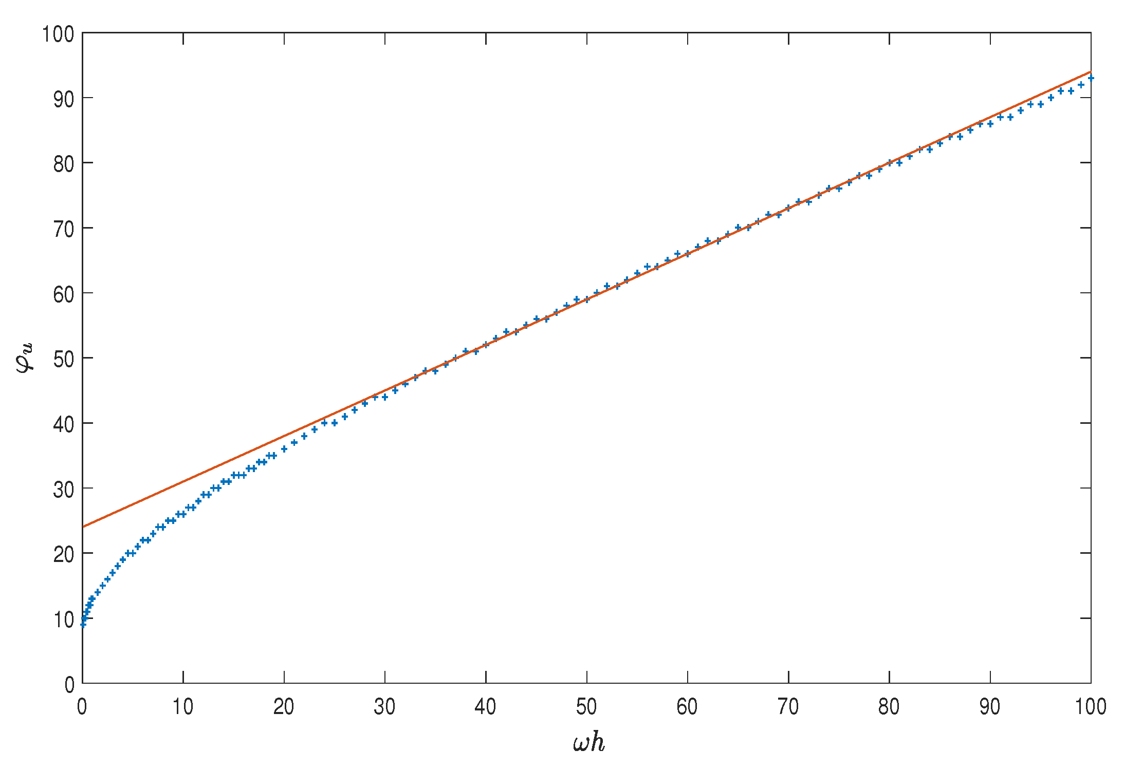
In so doing, one implicitly defines a function
, depending on the machine epsilon
u, such that
The plot of such a function is depicted in
Figure 2 for the double precision IEEE: as one may see, the function is well approximated by the line [
27]
Next, one consider the whole problem (
97), whose solution, on the interval
, can be written as
As observed before, when using a finite precision arithmetic with machine epsilon
u, the best we can do is to approximate (
106) with a polynomial:
provided that
Assuming the
ansatz , for a suitable
(essentially, one requires that
is well approximated by a polynomial of degree
), the requirement (
109) is accomplished by choosing ([
27], Criterion 2)
where
is the same function considered in (
104). By taking into account that
and that
is an increasing funcion (see
Figure 2), one then obtains that
.
Next, one has to approximate the Fourier coefficients (see (107))
,
, needed in (
108): for this purpose, we consider the Gauss-Legendre quadrature formula of order
. In order to gain full machine accuracy, when using the double precision IEEE, according to [
27], we choose
In so doing, we arrive to a HBVM
method. For such a method, the blended iteration (
45) can be made extremely efficient by approximating the Jacobian of (
97) with its linear part (this has been already done when solving Hamiltonian PDEs, see (
92)), so that the matrix
in (
44) has to be computed only once. Moreover, since we are going to use relatively large stepsizes
h, the initial guess for the vector
in (
45) is chosen, by considering the polynomial
defined in (
100) derived from the linear problem (
98), as:
The name
spectral HBVM with parameters has been coined in [
27] to denote the resulting method, in short
SHBVM. In order to show its effectiveness, we report here some numerical results obtained by solving the Duffing equation
with Hamiltonian
and exact solution
Here,
is the elliptic Jacobi function, with elliptic modulus specified by the second argument. In particular, we choose the values
providing a problem in the form (
94) to (
95), with a corresponding Hamiltonian value
. For solving it, we shall use the SHBVM method with parameters:
and a time-step
, for various values of
N, as specified in
Table 4. In that table we also list the corresponding:
maximum absolute error in the computed solution, ;
the maximum relative error in the numerical Hamiltonian, ;
the value of (which is always much greater than 1);
the parameters
, computed according to (
104), (
110), and (
111), respectively;
the execution time (in sec).
As before, the numerical tests have been performed on a laptop with a 2.2 GHz dual core i7 processor, 8 GB of memory, and running Matlab R2017b.
As one may see, the method is always energy conserving and the error, as expected, is uniformly small. Also the execution times are all very small (of the order of 3.5 s). It must be emphasized that classical methods, such as the Gautschi or the Deuflhard method, would require the use of much smaller time-steps, and much larger execution times (we refer to [
27] for some comparisons).


