Abstract
In this paper, we study the class of mixed-index time fractional differential equations in which different components of the problem have different time fractional derivatives on the left-hand side. We prove a theorem on the solution of the linear system of equations, which collapses to the well-known Mittag–Leffler solution in the case that the indices are the same and also generalises the solution of the so-called linear sequential class of time fractional problems. We also investigate the asymptotic stability properties of this class of problems using Laplace transforms and show how Laplace transforms can be used to write solutions as linear combinations of generalised Mittag–Leffler functions in some cases. Finally, we illustrate our results with some numerical simulations.
1. Introduction
Time fractional and space fractional differential equations are increasingly used as a powerful modelling tool for understanding the role of heterogeneity in the modulating function in such diverse areas as cardiac electrophysiology [1,2,3], brain dynamics [4], medicine [5], biology [6,7], porous media [8,9] and physics [10]. Time fractional models are typically used to model subdiffusive processes (anomalous diffusion [11,12]), while space fractional models are often associated with modelling processes occurring in complex spatially heterogeneous domains [1].
Time fractional models typically have solutions with heavy tails as described by the Mittag–Leffler matrix function [13] that naturally occurs when solving time fractional linear systems. However, such models are usually only described by a single fractional exponent, , associated with the fractional derivative. The fractional exponent can allow the coupling of different processes that may be occurring in different spatial domains by using different fractional exponents for the different regimes. One natural application here would be the coupling of models describing anomalous diffusion of proteins on the plasma membrane of the cell with the behaviour of other proteins in the cytosol of the cell. Tian et al. [14] addressed this problem by coupling a stochastic model (based on the stochastic simulation algorithm [15]) for the plasma membrane with systems of ordinary differential equations describing reaction cascades within the cell. It may also be necessary to couple more than two models, and so, in this paper, we introduce a formulation that focuses on coupling an arbitrary number of domains in which dynamical processes are occurring described by different anomalous diffusive processes. This leads us to consider the r index time fractional differential equation problem in Caputo form:
or in vector form:
Here, are matrices, while A is the associated block matrix of dimension , and has all components .
We believe that a modelling approach based on this formulation has not been fully developed before. We note that scalar linear sequential fractional problems have been considered whose solution can be described by multi-indexed Mittag–Leffler functions [16], and there are a number of articles on the numerical solution of multi-term fractional differential equations [17,18,19,20,21,22]. While mixed index problems can, in some cases, be written in the form of linear sequential problems, namely , we claim that it is inappropriate to do so in many cases. We note that Diethelm et al. [20] have very recently considered the asymptotic behaviour of certain linear multi-order fractional differential equations from a theoretical viewpoint.
Therefore, in this paper, we develop a new theorem that gives the analytical solution of equations such as (1) that reduces to the Mittag–Leffler expansion in the case that all the indices are the same (Section 3) and generalises the class of linear sequential problems (Section 3.1). We then analyse the asymptotic stability properties of these mixed index problems using Laplace transform techniques (Section 3.2), relating our results with known results that have been developed in control theory. In Section 3.2, we also show that, in the case that the are all rational, the solutions to the linear problem can be written as a linear combination of generalised Mittag–Leffler functions, again using ideas from control theory and transfer functions. In Section 4, we present some numerical simulations illustrating the results in this paper and give some discussion on how these ideas can be used to solve semi-linear problems either by extending the methodology of exponential integrators to Mittag–Leffler functions or by writing the solution as sums of certain Mittag–Leffler expansions.
2. Materials and Methods
2.1. Analytical Solutions
We consider the linear system given in (1) with and . It will be convenient to let:
where A is We will call such a system a time fractional index-2 system. Here, the Caputo time fractional derivative with starting point at is defined (see Podlubny [23], for example), as:
Furthermore, given a fixed mesh of size h, then a first order approximation of the Caputo derivative [24] is given by:
If = , then the solution to (1) is given by the Mittag–Leffler expansion:
where is the Gamma function.
In order to solve (4), this requires us to solve problems of the form:
Before making further headway, we need some additional background material.
Definition 1.
Generalisations of the Mittag–Leffler functions are given by:
where is the Pochhammer symbol:
see [22]. We will only consider the case where γ is a positive integer, but it can take on positive real values.
Remark 1.
The following Lemmas are standard results; see [16,23], for example.
Lemma 1.
Lemma 2.
The Laplace transform of satisfies:
Lemma 3.
The Caputo derivatives satisfy the following relationships.
- (i)
- (ii)
- (iii)
Lemma 4.
The solution of the scalar, linear, non-homogeneous problem:
is:
Note, it is insightful that this can be proven using the integral form from Lemma 3, namely:
We now apply a Picard-style iteration of the form:
where . Then, the iteration will converge to (8).
Lemma 5.
Proof
Use Definition 1, and integrate the left-hand side term by term. ☐
Remark 2.
The function multiplying in the integrand of (8), namely:
can be viewed as a Green function. For example, when ,
The generalisation of the class of problems given by (7) to the systems case takes the form:
In the case that , the solution of the linear homogeneous system is:
We have the following theorem (see Podlubny [23]):
Theorem 1.
The solution of (9) is given by:
2.2. Asymptotic Stability of Multi-Index Systems
The first contribution to the asymptotic stability analysis of time fractional linear systems was by Matignon [25]. Given the linear system in Caputo form, then taking the Laplace transform and using the definition of the Caputo derivative give:
or:
Here, is the Laplace transform of . If we write then the matrix will be nonsingular if w is not an eigenvalue of A. In the w-domain, this will happen if , where denotes the spectrum of A. In the s-domain, this will happen if That is, the eigenvalues of A lie in the complex plane minus the sector subtended by angle symmetric about the positive real axis; see Figure 1.
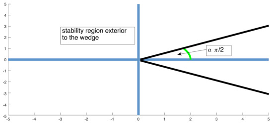
Figure 1.
Asymptotic stability region for single index scalar problem, for complex values of (imaginary, vertical axis; real, horizontal axis).
In fact, Laplace transforms are a very powerful technique for studying the asymptotic stability of mixed index fractional systems. Deng et al. [26] studied the stability of linear time fractional systems with delays using Laplace transforms. Given the delay system:
then the Laplace transform results in:
Hence, Deng et al. [26] proved:
Theorem 2.
If all the zeros of the characteristic polynomial of have a negative real part, then the zero solution of (13) is asymptotically stable.
Deng et al. [26] also proved a very nice result in the case that all the indices are rational.
Theorem 3.
Consider (13) with no delays and all the and are rational. In particular, let:
Then, let M be the lowest common multiple of all the denominators, and set . Then, the problem will be asymptotically stable if all the roots, λ, of:
satisfy
Remark 3.
If , then Theorem 3 reduces to the result of Matignon. The proof of Theorem 3 comes immediately from (14), where is the characteristic polynomial of .
Remark 4.
A nice survey on the stability (both linear and nonlinear) of fractional differential equations is given in Li and Zhang [27], while Saberi Najafi et al. [28] have extended some of these stability results to distributed order fractional differential equations with respect to an order density function. Zhang et al. [29] consider the stability of nonlinear fractional differential equations.
Remark 5.
Radwan et al. [30] note that the stability analysis of mixed index problems reduces to the study of the roots of the characteristic equation:
In the case that the are arbitrary real numbers, the study of the roots of (15) is difficult. By letting , we can cast this in the framework of quasi (or exponential) polynomials (Rivero et al. [31]). The zeros of exponential polynomials have been studied by Ritt [32].
The general form of an exponential polynomial with constant coefficients is:
An analogue of the fact that a polynomial of degree k can have up to k roots is expressed by a theorem due to Tamarkin, Pólya and Schwengler (see [32]).
Theorem 4.
Let P be the smallest convex polygon containing the values , and let the sides of P be . Then, there exist k half strips with half rays parallel to the outer normal to that contain all the zeros of f. If is the length of , then the number of zeros in the i-th half strip with modulus less than or equal to r is asymptotically
3. Results
3.1. The Solution of Mixed Index Linear Systems
The main focus of this paper is to consider generalisations of (9), where the vector has different components. In its general form, we will let where and . We will also assume and that A can be written in block form . We will also let and consider a class of linear, non-homogeneous multi-indexed systems of FDEs of the form:
that we interpret as the system:
The index of the system is said to be r.
In the case that , then by letting:
Thus, in the case that all , so that the individual components are scalar and so , (18) implies
For example, when , this becomes:
or
while for this gives, after some simplification,
Clearly, there is a general formula for arbitrary r in terms of the cofactors of A. In particular, it can be fitted into the framework of linear sequential FDEs [16,23,24,33,34]. These take the form:
However, this characterisation is not particularly simple, useful or computationally expedient. Furthermore, when the are not one, so that the individual components are not scalar, then there is no simple representation such as (19), and new approaches are needed. Before we consider this new approach, we note the converse, namely that (19) can always be written in the form of (16) for a suitable matrix A with a special structure. In particular, we can write (19) in the form of (16) with as an r dimensional, r index problem with and:
For completeness: we note in the case that and , an explicit solution to this problem was given in Podlubny [23]. This can be found by considering the transfer function (see Section 3.2) given by:
By finding the poles of this function and converting back to the untransformed domain, Podlubny gives the solution as:
where:
We now return to the index-2 problem (1) and (2). We first claim that the solution takes the matrix form:
where the are appropriate matrices, of size and respectively, that are to be determined.
We now use the fact that:
In order to get a succinct representation of the solution based on (20) and (25), it will be convenient to write:
so , and let .
We will also define the matrices:
where 0 represents appropriately-sized zero matrices. Now, we note that the recursive relation (25) is equivalent to:
Thus, we can state the following theorem.
Theorem 5.
The solution of the fractional index-2 system:
is given by:
where for :
Remark 6.
Remark 7.
Remark 8.
If the fractional index-2 system has initial condition , then the solution is:
We note that in solving (9), an equivalent solution to (11) is:
where is the Green function satisfying:
This leads us to give a general result on the solution of the mixed index problem (9) (with ) with a time-dependent forcing function, but first, we need the following definition.
Definition 2.
Let , then define:
Theorem 6.
The solution to the fractional index-2 problem:
is given by:
Proof
The result follows from together with the above discussion. ☐
We now turn to analysing the asymptotic stability of linear fractional index-2 systems.
3.2. Study of Asymptotic Stability
Recalling Theorem 4, we note that if the are rational and with M the lowest common multiple of the denominators, this reduces to the polynomial:
This leads us to think about stability from a control theory point of view. Thus, given the system:
where:
then the solution of (34) can be written in terms of the transfer function:
where s is the Laplace variable (see Rivero et al. [31] and Petras [35]).
In the case of the so-called commensurate form in which:
then:
Cěrmák and Kisela [36] considered the specific problem:
where real In this case, the appropriate stability polynomial is , where . Based on Theorem 3, (37) is asymptotically stable if all the roots of satisfy .
By setting and substituting into and equating real and imaginary parts, it is easily seen that:
This leads to the following result, given in Cěrmák and Kisela [36].
Theorem 7.
Equation (37) is asymptotically stable with real and rational if:
We now follow this idea, but for arbitrarily-sized systems in our mixed index format, and this leads to slight modifications to (37). We first make a slight simplification and take , and we also assume that is nonsingular, then Problem (1) leads to:
and substituting into the equation for gives:
This leads us to consider the roots of the characteristic function:
In the scalar case, this gives an extension to (37) where the characteristic equation is:
This can be written in systems form as:
where:
or alternatively as:
This can now be considered as a generalised eigenvalue problem. From (40), we require to be nonsingular. That is:
Let us write and assume and that is nonsingular, so that from the previous analysis, this means:
Hence:
In order to make this more specific, let and:
Note that Then, (43) becomes:
If we now assume that:
which defines the asymptotic stability boundary (the imaginary axis) when then (46) becomes:
Hence:
Equations (48) and (49) will define the asymptotic stability boundary with as a function of d. Rewriting (48) as:
and substituting (49) leads after simplification to:
Using the relationships:
gives:
Furthermore, we can write (50) as:
Thus, we have proven the following result.
Theorem 8.
Given the mixed index problem with A as in (44), the angle for asymptotic stability satisfies:
or in radians with :
with the minimum occurring with:
Remark 9.
We have the following results for in three particular cases:
- (i)
- , since in this case, .
- (ii)
- . In the case , we see from (52) that:Letting with small, then . This means that , as a function of r, is very shallow apart from when r is near the origin or very large. Hence, the asymptotic stability boundary will be almost constant over long periods of d when α and β are close together.
- (iii)
Due to the nonlinearities in (57), it is hard to determine an explicit simple relation between and d except if . In this case, we make use of the following Lemma.
Lemma 6.
If and , then there is a solution:
Proof
This is by subtraction of the two equations and substitution. ☐
Hence:
Note that:
and:
Some manipulation of(59) leads to:
Now, since , this reduces to:
By taking . this gives an explicit relationship between and d for the case .
Remark 10.
Particular solutions are:
- (i)
- (ii)
It is clear from (60) that when and , then , and then, the angle will make an excursion from down to a minimum value and back to as d increases. For example, in the case of , we can see from Remark 10(i) that the minimum value of the angle is when:
Now, if and are rational :
and with then:
From Descartes’ rule of sign, then (62) will have at most four real zeros if is even, and at most five real zeros if is odd.
Now, factorise:
where there are at most four real zeros if N is even and at most five real zeros if N is odd. Then, using (63) and (64), we can write:
where the can be found by writing:
where:
Using Lemma 2 with:
leads to the following result.
Theorem 9.
The solution of the mixed index-2 problem with , all positive integers is, with , given by:
where the are the zeros of (62) and the are the coefficients in the partial fraction expansion.
Remark 11.
In the case that , then (65) should collapse to the solution:
and this is not immediately clear. However, in this case, , and so:
which is a quadratic function in while the equivalent and numerator functions are linear in . Thus, in (65), N is replaced by two, is replaced by α and becomes one. Thus, (65) reduces to:
that then becomes (66). On the other hand, if α is rational and then:
If we factorise:
and find by:
then we have the following Corollary.
Corollary 1.
The solution of the mixed index-2 problem with α rational and , K a positive integer is given by:
where the vectors and “eigenvalues” satisfy (68).
As a particular example, take then the and in Corollary 1 satisfy:
and:
In other words:
or:
with:
Clearly, in the case described by Corollary 1, writing the solution as a linear combination of generalised Mittag–Leffler functions makes the evaluation of the solution much more computationally efficient.
4. Simulations and Discussion
In this section, we give a variety of asymptotic stability and dynamics results for different parameter values of the linear mixed index models.
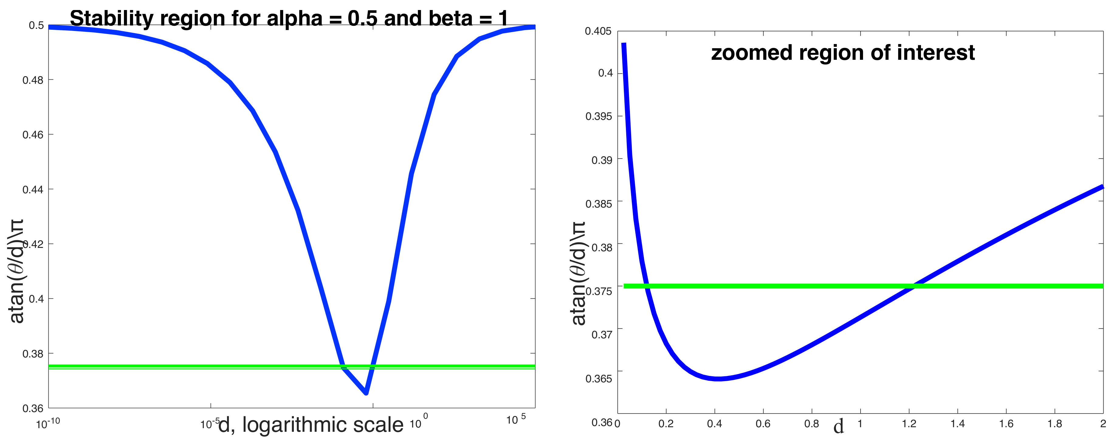
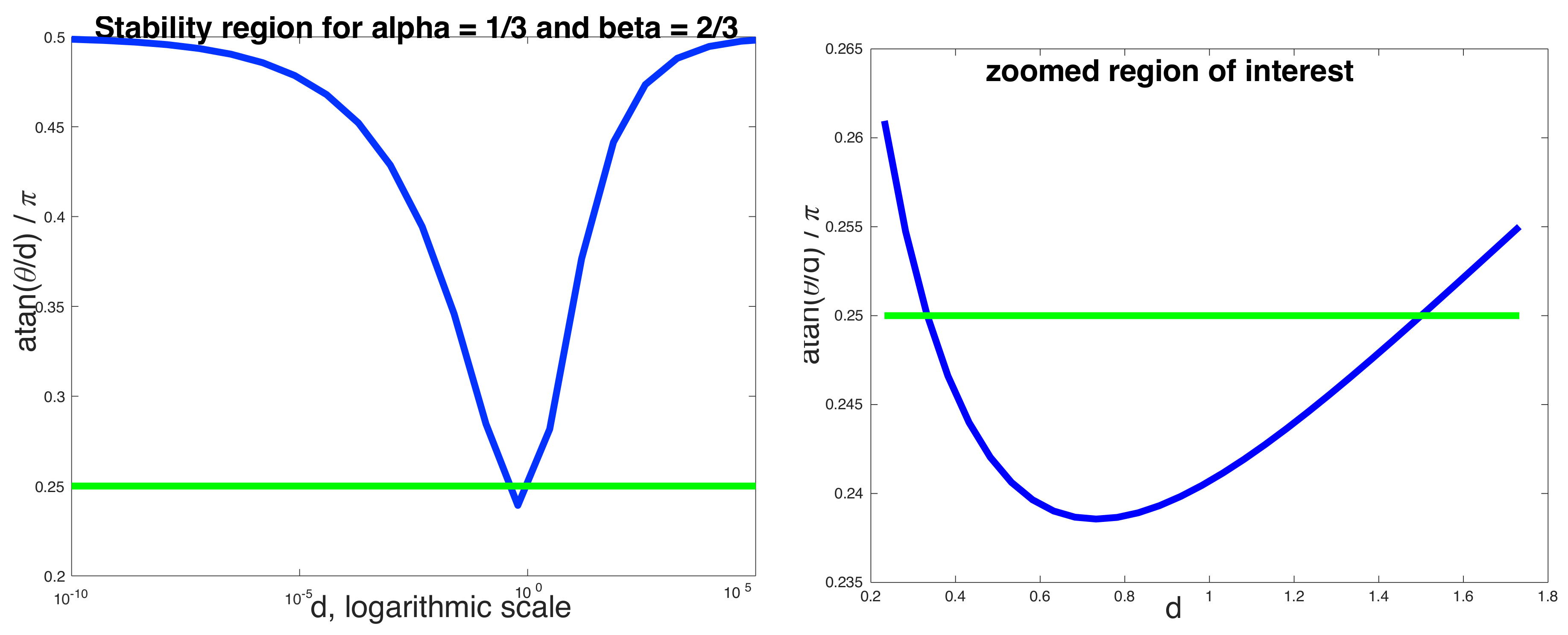
In Figure 2 and Figure 3, we plot the asymptotic stability boundary of the two dimensional, index-2 problem given by (1) where:
for the two cases considered in Section 3.2, namely (Figure 2) and (Figure 3). Since the eigenvalues of A are , we plot on the vertical axis the angle in radians, where , as a function of d. In Figure 2, we see that corresponding to an angle lying between 45° and 90°, as expected from the theory. We also plot the angle, in green, corresponding to the midpoint between these two extremes, i.e., . We see that for the most part, the asymptotic stability angle lies above this midpoint, except for the values of d, as shown in the right-hand figure.
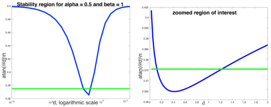
Figure 2.
Stability region, above the blue line, for choosing d and , when the eigenvalues of A are , The logarithmic scale is explored in the right-hand figure where the stability boundary dips below the angle .

Figure 3.
Stability region, above the blue line, for choosing d and , when the eigenvalues of A are , The logarithmic scale is explored in the right-hand figure where the stability boundary dips below the angle .
In the case of Figure 3, we give a similar plot as Figure 2. We also plot in green the midpoint between the two lines subtended by angles and , namely . As with Figure 2, there is a small range of d for which the asymptotic stability angle drops beneath . Furthermore, it is clear from Remark 9(ii) that as and approach one another, the asymptotic stability boundary will be almost constant over increasingly longer periods of d and will only asymptotically approach the angle for very small and very large values of d.
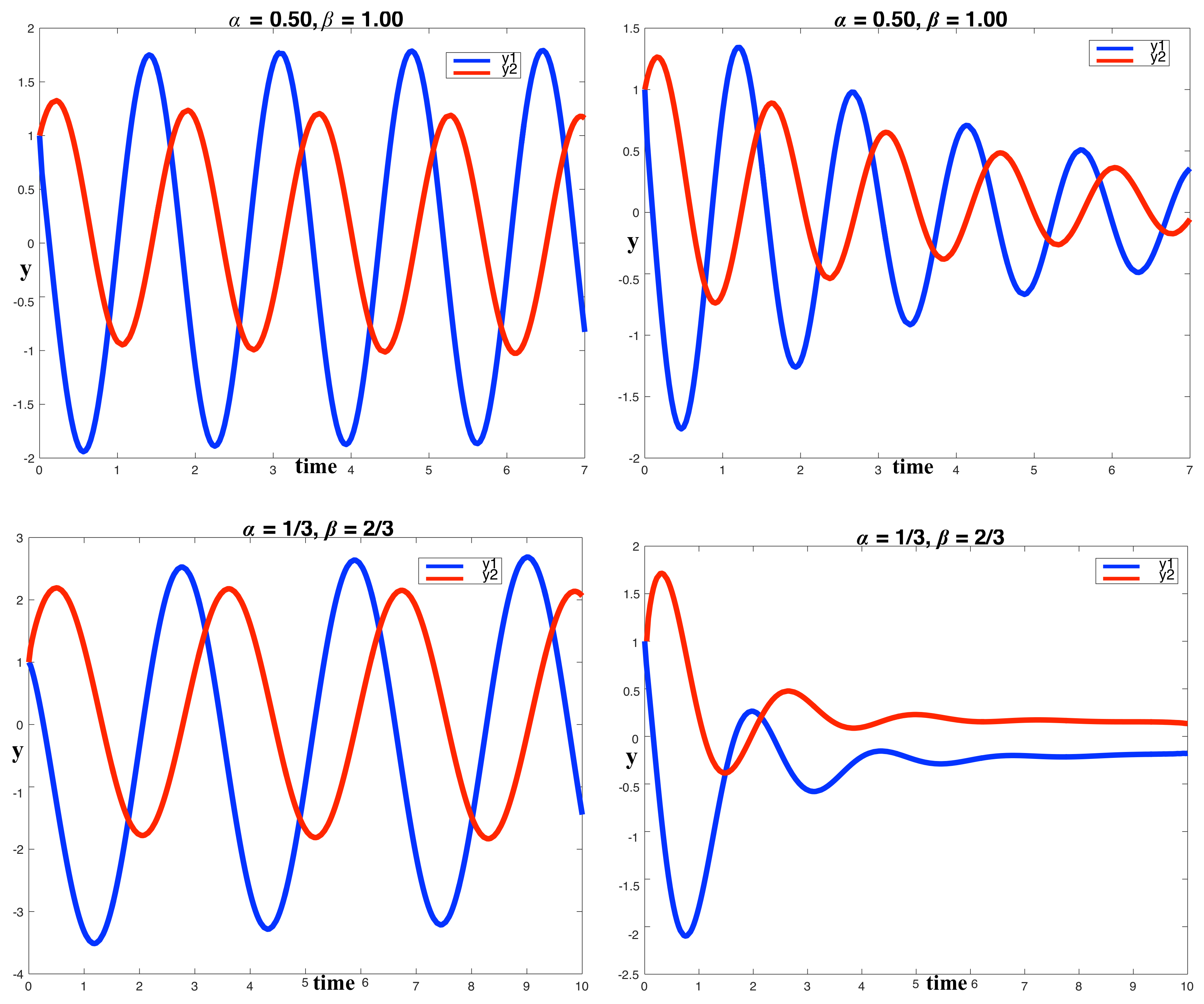
In Figure 4, we confirm the asymptotic stability analysis showing sustained and decaying oscillations with (top panel) and (bottom panel). In all four cases, , while for the top panel, we take , while for the bottom panel we take .
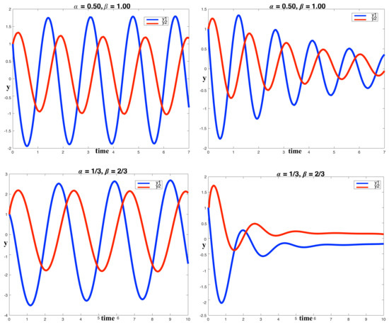
Figure 4.
System dynamics with , top, and , bottom. The left-hand column shows sustained dynamics with and chosen so that lies on the stability boundary. The right-hand column corresponds to the same d, but 0.3 has been added to the value.
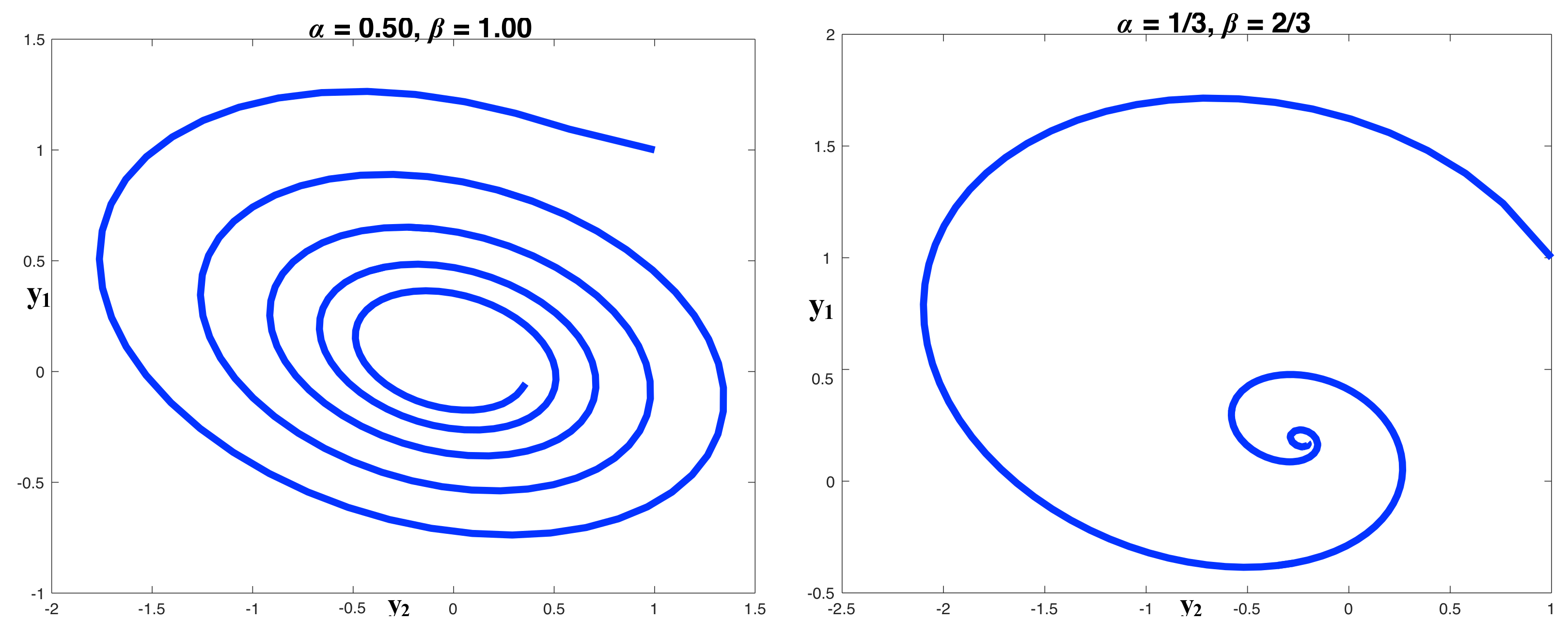
In Figure 5, we present phase plots of versus for the two decaying oscillations cases. The figures confirm our theoretical results on the asymptotic stability boundary and also show the effects that the fractional indices have on the period of the solutions. As approaches , we expect the oscillatory behaviour to disappear.
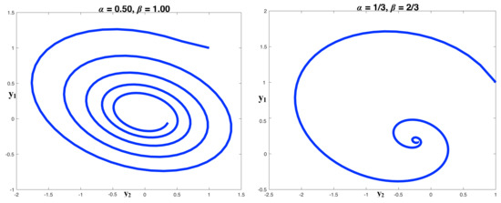
Figure 5.
Phase plots of versus for the decaying solutions in the right-hand column of Figure 4.
Finally, in Figure 6, we consider the problem:
in which case the eigenvalues of A are . We take and present the solutions for four pairs of indices, namely , . The simulations show that the components of the solution and seem to pick up “energy” from one another due to the coupling and that as the distance between and grows, there is a greater separation between the two components. Finally, as gets smaller, the solutions appear to “flat-line” more quickly.
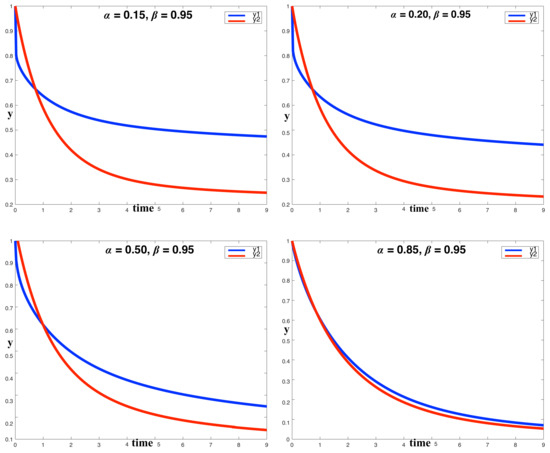
Figure 6.
For A given by (70) with so that the eigenvalues are , showing the effect of variation of with fixed on the system dynamics.
5. Conclusions
In this paper, we have studied mixed index fractional differential equations with coupling between the different components. We find an analytical expression for the solution of the linear system that generalises the Mittag–Leffler expansion of a matrix and the solution of linear sequential fractional differential equations. We can use this result to derive new numerical methods that generalise the concept of exponential methods used in the approximation of the Mittag–Leffler matrix function (see [37,38,39], for example) and exponential integrators [40,41]. The second element would deal with developing numerical techniques for the integration component that incorporates the integral of a function times a Green function. We also use Laplace transform techniques to find the asymptotic stability domain in terms of the eigenvalues of the defining linear system. Finally, we have also used Laplace transforms to get analytical expansions of the mixed index problem in terms of a sum of Mittag–Leffler or generalised Mittag–Leffler functions, in the case that the fractional indices are rational.
Acknowledgments
We would like to thank Alfonso Bueno-Orovio in the Department of Computer Science, University of Oxford, for many discussions about fractional differential equations. We also acknowledge the funding support from the ARC Centre of Excellence for Mathematical and Statistical Frontiers.
Author Contributions
All authors contributed equally.
Conflicts of Interest
The authors declare no conflict of interest.
References
- Bueno-Orovio, A.; Kay, D.; Grau, V.; Rodriguez, B.; Burrage, K. Fractional diffusion models of cardiac electrical propagation: Role of structural heterogeneity in dispersion of repolarization. J. R. Soc. Interface 2014, 11, 20140352. [Google Scholar] [CrossRef] [PubMed]
- Cusimano, N.; Bueno-Orovio, A.; Turner, I.; Burrage, K. On the order of the fractional Laplacian in determining the spatio-temporal evolution of a space-fractional model of cardiac electrophysiology. PLoS ONE 2015, 10, e0143938. [Google Scholar] [CrossRef] [PubMed]
- Bueno-Orovio, A.; Teh, I.; Schneider, J.E.; Burrage, K.; Grau, V. Anomalous diffusion in cardiac tissue as an index of myocardial microstructure. IEEE Trans. Med. Imaging 2016, 35, 2200–2207. [Google Scholar] [CrossRef] [PubMed]
- Henry, B.; Langlands, T. Fractional cable models for spiny neuronal dendrites. Phys. Rev. Lett. 2008, 100, 128103. [Google Scholar] [CrossRef] [PubMed]
- Magin, R.; Feng, X.; Baleanu, D. Solving the fractional order Bloch equation. Concepts Magn. Reson. Part A 2009, 34, 16–23. [Google Scholar] [CrossRef]
- Klafter, J.; White, B.; Levandowsky, M. Microzooplankton feeding behavior and the Lévy walk. In Biological Motion; Lecture Notes in Biomathematics; Springer: Berlin/Heidelberg, Germany, 1990; Volume 89, pp. 281–296. [Google Scholar]
- Cusimano, N.; Burrage, K.; Burrage, P. Fractional models for the migration of biological cells in complex spatial domains. ANZIAM J. 2013, 54, 250–270. [Google Scholar] [CrossRef][Green Version]
- Shen, S.; Liu, F.; Liu, Q.; Anh, V. Numerical simulation of anomalous infiltration in porous media. Numer. Algorithms 2015, 68, 443–454. [Google Scholar] [CrossRef]
- Carcione, J.; Sanchez-Sesma, F.; Luzon, F.; Gavilan, J.P. Theory and simulation of time-fractional fluid diffusion in porous media. J. Phys. A 2013, 46, 345501. [Google Scholar] [CrossRef]
- Metzler, R.; Klafter, J.; Sokolov, I.M. Anomalous transport in external fields: Continuous time random walks and fractional diffusion equations extended. Phys. Rev. E 1998, 58, 1621–1633. [Google Scholar] [CrossRef]
- Klages, R.; Radons, G.; Sokolov, I. Anomalous Transport; Wiley-VCH Verlag GmbH & Co.: Hoboken, NJ, USA, 2008. [Google Scholar]
- Metzler, R.; Klafter, J. The random walk’s guide to anomalous diffusion: A fractional dynamics approach. Phys. Rep. 2000, 339, 1–77. [Google Scholar] [CrossRef]
- Mittag–Leffler, G.M. Sur la nouvelle function Ea. C. R. Acad. Sci. 1903, 137, 554–558. [Google Scholar]
- Tian, T.; Harding, A.; Inder, K.; Parton, R.G.; Hancock, J.F. Plasma membrane nanoswitches generate high-fidelity Ras signal transduction. Nat. Cell Biol. 2007, 9, 905–914. [Google Scholar] [CrossRef] [PubMed]
- Gillespie, D.T. Exact stochastic simulation of coupled chemical reactions. J. Phys. Chem. 1977, 81, 2340–2361. [Google Scholar] [CrossRef]
- Kilbas, A.; Srivastava, H.M.; Trujillo, J.J. Theory and Applications of Fractional Differential Equations, North-Holland Mathematics Studies; Elsevier: Amsterdam, The Netherlands, 2006; Volume 204. [Google Scholar]
- Yu, Q.; Liu, F.; Turner, I.; Burrage, K. Numerical simulation of the fractional Bloch equations. J. Comp. Appl. Math. 2014, 255, 635–651. [Google Scholar] [CrossRef]
- Liu, F.; Meerschaert, M.M.; McGough, R.; Zhuang, P.; Liu, Q. Numerical methods for solving the multi-term time fractional wave equations. Fract. Calc. Appl. Anal. 2013, 16, 9–25. [Google Scholar] [CrossRef] [PubMed]
- Qin, S.; Liu, F.; Turner, I.; Yu, Q.; Yang, Q.; Vegh, V. Characterization of anomalous relaxation using the time-fractional Bloch equation and multiple echo T2*-weighted magnetic resonance imaging at 7T. Magn. Reson. Med. 2017, 77, 1485–1494. [Google Scholar] [CrossRef] [PubMed]
- Diethelm, K.; Siegmund, S.; Tuan, H.T. Asymptotic behavior of soutions of linear multi-order fractional differential systems. Fract. Calc. Appl. Anal. 2017, 20, 1165–1195. [Google Scholar] [CrossRef]
- Popolizio, M. Numerical solution of multiterm fractional differential equations using the matrix Mittag–Leffler functions. Mathematics 2018, 6, 7. [Google Scholar] [CrossRef]
- Prabhakar, T.R. A singular integral equation with a generalised Mittag–Leffler function in the kernel. Yokohama Math. J. 1971, 19, 7–15. [Google Scholar]
- Podlubny, I. Fractional Differential Equations; Academic Press: New York, NY, USA, 1999. [Google Scholar]
- Oldham, K.B.; Spanier, J. The Fractional Calculus: Theory and Applications of Differentiation and Integration to Arbitrary Order; Academic Press: New York, NY, USA, 1974. [Google Scholar]
- Matignon, D. Stability result on fractional differential equations with applications to control processing. In Proceedings of the July 1996 IMACS-SMC, Lille, France, July 1998; pp. 963–968. [Google Scholar]
- Deng, W.; Li, C.; Lu, J. Stability analysis of linear fractional differential system with multiple time delays. Nonnlinear Dyn. 2007, 48, 409–416. [Google Scholar] [CrossRef]
- Li, C.P.; Zhang, F.R. A survey on the stability of fractional differential equations. Eur. Phys. J. Spec. Top. 2011, 193, 27–47. [Google Scholar] [CrossRef]
- Najafi, H.S.; Sheikhani, A.R.; Ansari, A. Stability analysis of distributed order Fractional Differential Equations. Abstr. Appl. Anal. 2011, 175323. [Google Scholar] [CrossRef]
- Zhang, F.; Li, C.; Chen, Y. Asymptotical stability of nonlinear fractional differential system with Caputo Derivative. Int. J. Differ. Equ. 2011, 2011, 635165. [Google Scholar] [CrossRef]
- Radwan, A.G.; Soliman, A.M.; Elwakil, A.S.; Sedeek, A. On the stability of linear systems with fractional-order elements. Chaos Solitons Fractal 2009, 40, 2317–2328. [Google Scholar] [CrossRef]
- Rivero, M.; Rogosin, S.V.; Machado, J.A.T.; Trujillo, J.J. Stability of Fractional Order Systems. Math. Probl. Eng. 2013, 356215. [Google Scholar] [CrossRef]
- Ritt, J.F. On the zeros of exponential polynomials. Trans. Am. Math. Soc. 1929, 31, 680–686. [Google Scholar] [CrossRef]
- Miller, K.S.; Ross, B. Fractional Green’s functions. Indian J. Pure Appl. Math. 1991, 22, 763–767. [Google Scholar]
- Vazquez, L. Fractional diffusion equations with internal degrees of freedom. J. Comp. Math. 2003, 21, 491–494. [Google Scholar]
- Petras, I. Stability of fractional order systems with rational orders: A survey. Fract. Calc. Appl. Anal. 2009, 12, 269–298. [Google Scholar]
- Cěrmák, J.; Kisela, T. Stability properties of two term fractional differential equations. Nonlinear Dyn. 2015, 80, 1673–1684. [Google Scholar] [CrossRef]
- Garrappa, R.; Popolizio, M. Evaluation of generalized Mittag–Leffler functions on the real line. Adv. Comput. Math. 2013, 39, 205–225. [Google Scholar] [CrossRef]
- Zeng, C.; Chen, Y.Q. Global Padé Approximations of the Generalized Mittag–Leffler Function and its Inverse. Fract. Calc. Appl. Anal. 2015, 18, 149–156. [Google Scholar] [CrossRef]
- Garrappa, R. Numerical evaluation of two and three parameters Mittag–Leffler functions. SIAM J. Numer. Anal. 2015, 53, 1350–1369. [Google Scholar] [CrossRef]
- Sidje, R.B. Expokit: A software package for computing matrix exponentials. ACM Trans. Math. Softw. 1998, 24, 130–156. [Google Scholar] [CrossRef]
- Hochbruck, M.; Ostermann, A. Exponential integrators. Acta Numer. 2010, 19, 209–286. [Google Scholar] [CrossRef]
© 2018 by the authors. Licensee MDPI, Basel, Switzerland. This article is an open access article distributed under the terms and conditions of the Creative Commons Attribution (CC BY) license (http://creativecommons.org/licenses/by/4.0/).


