On the Analysis of Mixed-Index Time Fractional Differential Equation Systems


Abstract
1. Introduction
2. Materials and Methods
2.1. Analytical Solutions
- (i)
- (ii)
- (iii)
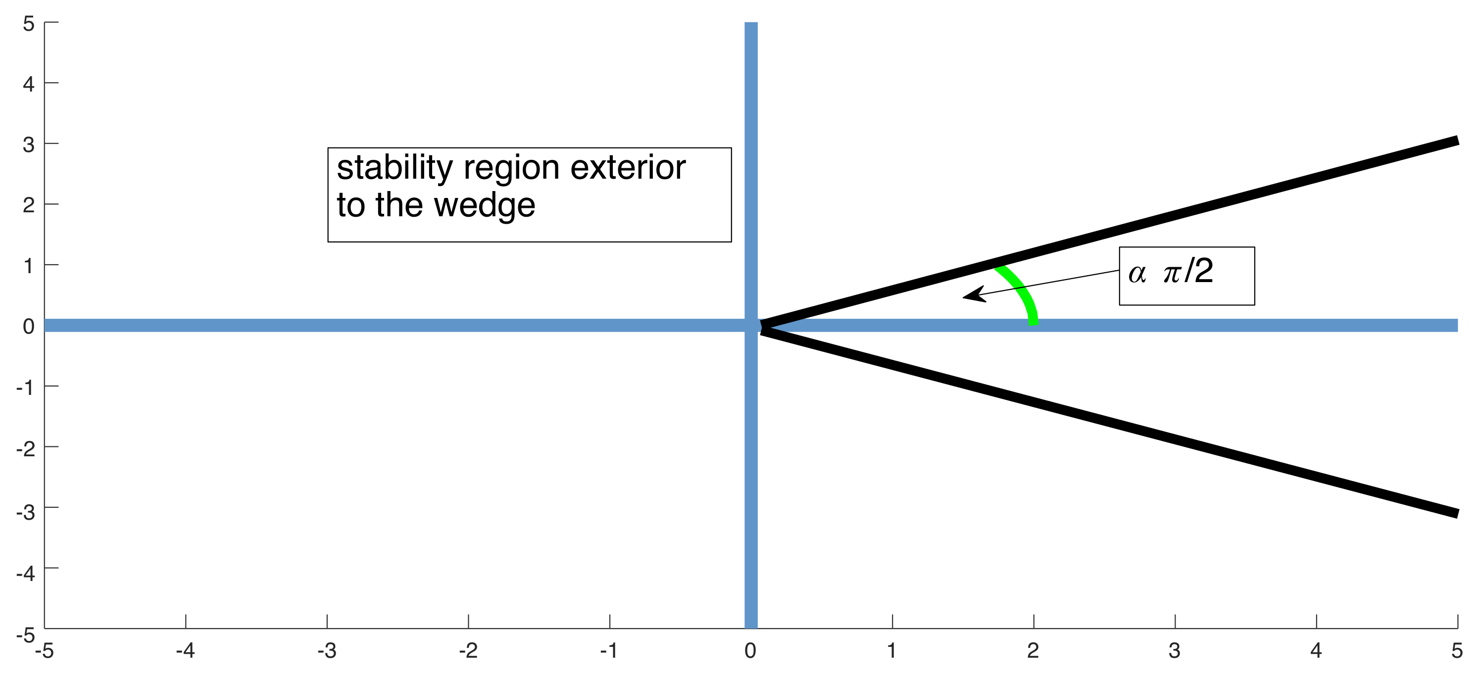
2.2. Asymptotic Stability of Multi-Index Systems
3. Results
3.1. The Solution of Mixed Index Linear Systems
3.2. Study of Asymptotic Stability
- (i)
- , since in this case, .
- (ii)
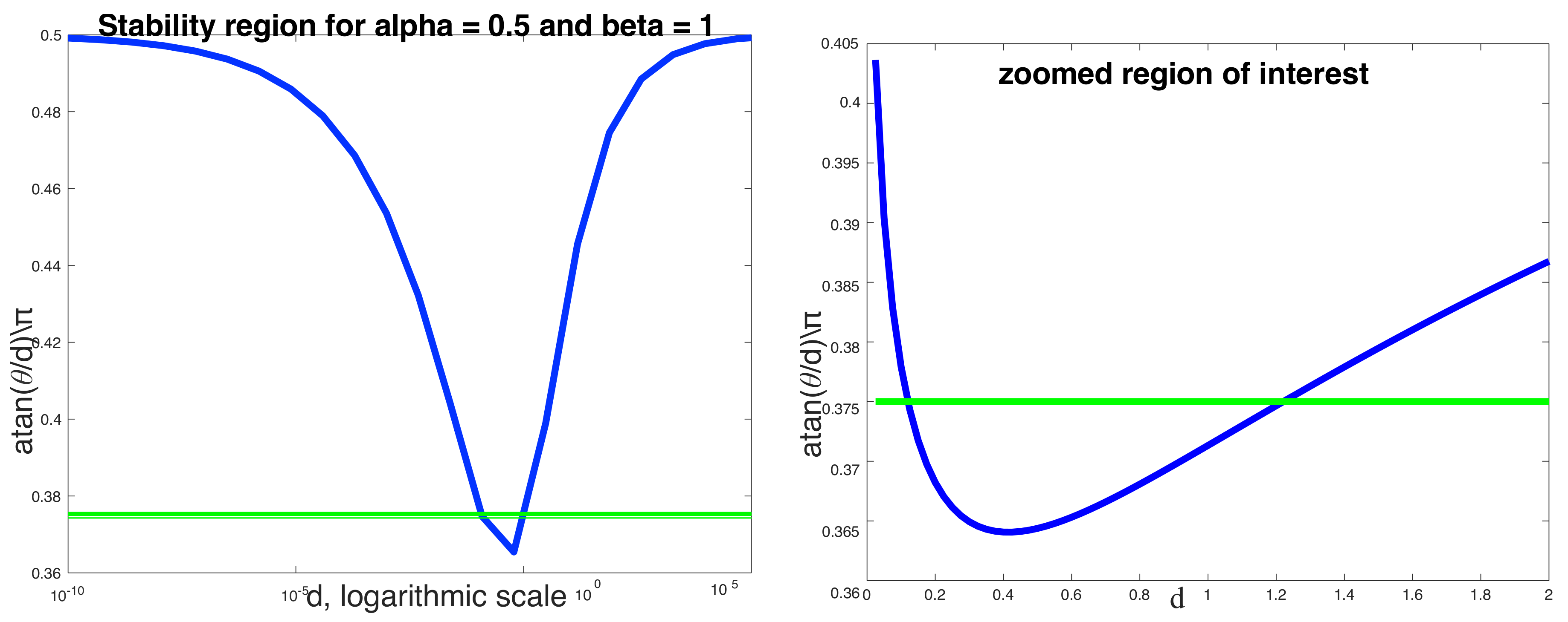
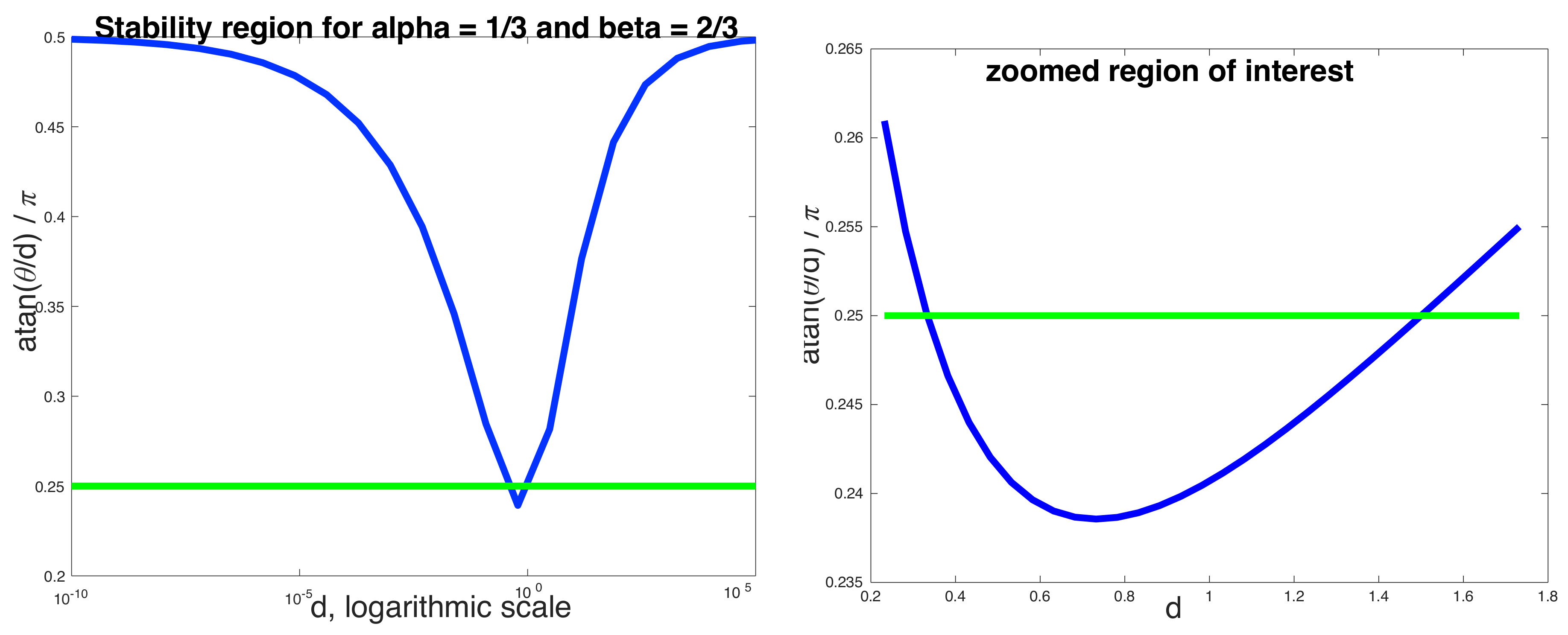
- . In the case , we see from (52) that:Letting with small, then . This means that , as a function of r, is very shallow apart from when r is near the origin or very large. Hence, the asymptotic stability boundary will be almost constant over long periods of d when α and β are close together.
- (iii)
- (i)
- (ii)
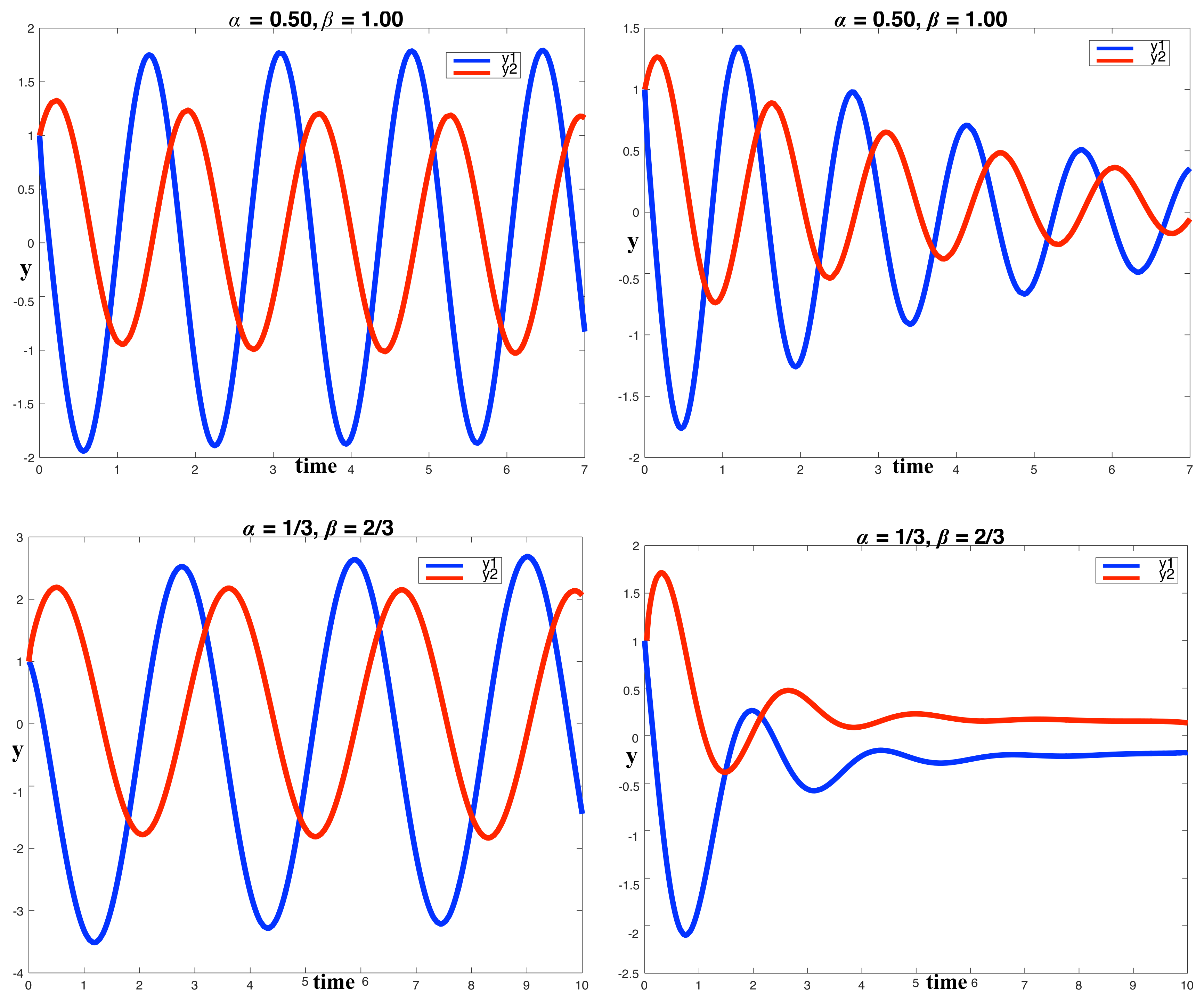
4. Simulations and Discussion
5. Conclusions
Acknowledgments
Author Contributions
Conflicts of Interest
References
- Bueno-Orovio, A.; Kay, D.; Grau, V.; Rodriguez, B.; Burrage, K. Fractional diffusion models of cardiac electrical propagation: Role of structural heterogeneity in dispersion of repolarization. J. R. Soc. Interface 2014, 11, 20140352. [Google Scholar] [CrossRef] [PubMed]
- Cusimano, N.; Bueno-Orovio, A.; Turner, I.; Burrage, K. On the order of the fractional Laplacian in determining the spatio-temporal evolution of a space-fractional model of cardiac electrophysiology. PLoS ONE 2015, 10, e0143938. [Google Scholar] [CrossRef] [PubMed]
- Bueno-Orovio, A.; Teh, I.; Schneider, J.E.; Burrage, K.; Grau, V. Anomalous diffusion in cardiac tissue as an index of myocardial microstructure. IEEE Trans. Med. Imaging 2016, 35, 2200–2207. [Google Scholar] [CrossRef] [PubMed]
- Henry, B.; Langlands, T. Fractional cable models for spiny neuronal dendrites. Phys. Rev. Lett. 2008, 100, 128103. [Google Scholar] [CrossRef] [PubMed]
- Magin, R.; Feng, X.; Baleanu, D. Solving the fractional order Bloch equation. Concepts Magn. Reson. Part A 2009, 34, 16–23. [Google Scholar] [CrossRef]
- Klafter, J.; White, B.; Levandowsky, M. Microzooplankton feeding behavior and the Lévy walk. In Biological Motion; Lecture Notes in Biomathematics; Springer: Berlin/Heidelberg, Germany, 1990; Volume 89, pp. 281–296. [Google Scholar]
- Cusimano, N.; Burrage, K.; Burrage, P. Fractional models for the migration of biological cells in complex spatial domains. ANZIAM J. 2013, 54, 250–270. [Google Scholar] [CrossRef][Green Version]
- Shen, S.; Liu, F.; Liu, Q.; Anh, V. Numerical simulation of anomalous infiltration in porous media. Numer. Algorithms 2015, 68, 443–454. [Google Scholar] [CrossRef]
- Carcione, J.; Sanchez-Sesma, F.; Luzon, F.; Gavilan, J.P. Theory and simulation of time-fractional fluid diffusion in porous media. J. Phys. A 2013, 46, 345501. [Google Scholar] [CrossRef]
- Metzler, R.; Klafter, J.; Sokolov, I.M. Anomalous transport in external fields: Continuous time random walks and fractional diffusion equations extended. Phys. Rev. E 1998, 58, 1621–1633. [Google Scholar] [CrossRef]
- Klages, R.; Radons, G.; Sokolov, I. Anomalous Transport; Wiley-VCH Verlag GmbH & Co.: Hoboken, NJ, USA, 2008. [Google Scholar]
- Metzler, R.; Klafter, J. The random walk’s guide to anomalous diffusion: A fractional dynamics approach. Phys. Rep. 2000, 339, 1–77. [Google Scholar] [CrossRef]
- Mittag–Leffler, G.M. Sur la nouvelle function Ea. C. R. Acad. Sci. 1903, 137, 554–558. [Google Scholar]
- Tian, T.; Harding, A.; Inder, K.; Parton, R.G.; Hancock, J.F. Plasma membrane nanoswitches generate high-fidelity Ras signal transduction. Nat. Cell Biol. 2007, 9, 905–914. [Google Scholar] [CrossRef] [PubMed]
- Gillespie, D.T. Exact stochastic simulation of coupled chemical reactions. J. Phys. Chem. 1977, 81, 2340–2361. [Google Scholar] [CrossRef]
- Kilbas, A.; Srivastava, H.M.; Trujillo, J.J. Theory and Applications of Fractional Differential Equations, North-Holland Mathematics Studies; Elsevier: Amsterdam, The Netherlands, 2006; Volume 204. [Google Scholar]
- Yu, Q.; Liu, F.; Turner, I.; Burrage, K. Numerical simulation of the fractional Bloch equations. J. Comp. Appl. Math. 2014, 255, 635–651. [Google Scholar] [CrossRef]
- Liu, F.; Meerschaert, M.M.; McGough, R.; Zhuang, P.; Liu, Q. Numerical methods for solving the multi-term time fractional wave equations. Fract. Calc. Appl. Anal. 2013, 16, 9–25. [Google Scholar] [CrossRef] [PubMed]
- Qin, S.; Liu, F.; Turner, I.; Yu, Q.; Yang, Q.; Vegh, V. Characterization of anomalous relaxation using the time-fractional Bloch equation and multiple echo T2*-weighted magnetic resonance imaging at 7T. Magn. Reson. Med. 2017, 77, 1485–1494. [Google Scholar] [CrossRef] [PubMed]
- Diethelm, K.; Siegmund, S.; Tuan, H.T. Asymptotic behavior of soutions of linear multi-order fractional differential systems. Fract. Calc. Appl. Anal. 2017, 20, 1165–1195. [Google Scholar] [CrossRef]
- Popolizio, M. Numerical solution of multiterm fractional differential equations using the matrix Mittag–Leffler functions. Mathematics 2018, 6, 7. [Google Scholar] [CrossRef]
- Prabhakar, T.R. A singular integral equation with a generalised Mittag–Leffler function in the kernel. Yokohama Math. J. 1971, 19, 7–15. [Google Scholar]
- Podlubny, I. Fractional Differential Equations; Academic Press: New York, NY, USA, 1999. [Google Scholar]
- Oldham, K.B.; Spanier, J. The Fractional Calculus: Theory and Applications of Differentiation and Integration to Arbitrary Order; Academic Press: New York, NY, USA, 1974. [Google Scholar]
- Matignon, D. Stability result on fractional differential equations with applications to control processing. In Proceedings of the July 1996 IMACS-SMC, Lille, France, July 1998; pp. 963–968. [Google Scholar]
- Deng, W.; Li, C.; Lu, J. Stability analysis of linear fractional differential system with multiple time delays. Nonnlinear Dyn. 2007, 48, 409–416. [Google Scholar] [CrossRef]
- Li, C.P.; Zhang, F.R. A survey on the stability of fractional differential equations. Eur. Phys. J. Spec. Top. 2011, 193, 27–47. [Google Scholar] [CrossRef]
- Najafi, H.S.; Sheikhani, A.R.; Ansari, A. Stability analysis of distributed order Fractional Differential Equations. Abstr. Appl. Anal. 2011, 175323. [Google Scholar] [CrossRef]
- Zhang, F.; Li, C.; Chen, Y. Asymptotical stability of nonlinear fractional differential system with Caputo Derivative. Int. J. Differ. Equ. 2011, 2011, 635165. [Google Scholar] [CrossRef]
- Radwan, A.G.; Soliman, A.M.; Elwakil, A.S.; Sedeek, A. On the stability of linear systems with fractional-order elements. Chaos Solitons Fractal 2009, 40, 2317–2328. [Google Scholar] [CrossRef]
- Rivero, M.; Rogosin, S.V.; Machado, J.A.T.; Trujillo, J.J. Stability of Fractional Order Systems. Math. Probl. Eng. 2013, 356215. [Google Scholar] [CrossRef]
- Ritt, J.F. On the zeros of exponential polynomials. Trans. Am. Math. Soc. 1929, 31, 680–686. [Google Scholar] [CrossRef]
- Miller, K.S.; Ross, B. Fractional Green’s functions. Indian J. Pure Appl. Math. 1991, 22, 763–767. [Google Scholar]
- Vazquez, L. Fractional diffusion equations with internal degrees of freedom. J. Comp. Math. 2003, 21, 491–494. [Google Scholar]
- Petras, I. Stability of fractional order systems with rational orders: A survey. Fract. Calc. Appl. Anal. 2009, 12, 269–298. [Google Scholar]
- Cěrmák, J.; Kisela, T. Stability properties of two term fractional differential equations. Nonlinear Dyn. 2015, 80, 1673–1684. [Google Scholar] [CrossRef]
- Garrappa, R.; Popolizio, M. Evaluation of generalized Mittag–Leffler functions on the real line. Adv. Comput. Math. 2013, 39, 205–225. [Google Scholar] [CrossRef]
- Zeng, C.; Chen, Y.Q. Global Padé Approximations of the Generalized Mittag–Leffler Function and its Inverse. Fract. Calc. Appl. Anal. 2015, 18, 149–156. [Google Scholar] [CrossRef]
- Garrappa, R. Numerical evaluation of two and three parameters Mittag–Leffler functions. SIAM J. Numer. Anal. 2015, 53, 1350–1369. [Google Scholar] [CrossRef]
- Sidje, R.B. Expokit: A software package for computing matrix exponentials. ACM Trans. Math. Softw. 1998, 24, 130–156. [Google Scholar] [CrossRef]
- Hochbruck, M.; Ostermann, A. Exponential integrators. Acta Numer. 2010, 19, 209–286. [Google Scholar] [CrossRef]


© 2018 by the authors. Licensee MDPI, Basel, Switzerland. This article is an open access article distributed under the terms and conditions of the Creative Commons Attribution (CC BY) license (http://creativecommons.org/licenses/by/4.0/).
Share and Cite
Burrage, K.; Burrage, P.; Turner, I.; Zeng, F. On the Analysis of Mixed-Index Time Fractional Differential Equation Systems. Axioms 2018, 7, 25. https://doi.org/10.3390/axioms7020025
Burrage K, Burrage P, Turner I, Zeng F. On the Analysis of Mixed-Index Time Fractional Differential Equation Systems. Axioms. 2018; 7(2):25. https://doi.org/10.3390/axioms7020025
Chicago/Turabian StyleBurrage, Kevin, Pamela Burrage, Ian Turner, and Fanhai Zeng. 2018. "On the Analysis of Mixed-Index Time Fractional Differential Equation Systems" Axioms 7, no. 2: 25. https://doi.org/10.3390/axioms7020025
APA StyleBurrage, K., Burrage, P., Turner, I., & Zeng, F. (2018). On the Analysis of Mixed-Index Time Fractional Differential Equation Systems. Axioms, 7(2), 25. https://doi.org/10.3390/axioms7020025