Bending Fields for Dual Curves

Abstract

This paper provides several new characterizations of the infinitesimal bending of dual curves, which is defined as an infinitesimal deformation preserving dual arc length (with appropriate precision). The main goal is to consider the infinitesimal deformations of ruled surfaces through the corresponding deformations of dual curves. Some useful properties of the infinitesimal bending of dual curves are obtained, and dual bending fields are determined. The Vekua-type characterization of the infinitesimal bending of dual curves is formulated in terms of the derivative of the dual arc length. Explicit formulas for dual infinitesimal bending fields of dual spherical curves are obtained using the Blaschke frame, considering both an arbitrary real parameter and the dual arc length. A necessary and sufficient condition for the infinitesimal bending of the dual curve to lie on the dual unit sphere is presented in terms of Blaschke and Frenet invariants. Several examples are illustrated graphically using our own software tool.

1. Introduction

The geometric study of curves and surfaces occupies a central position in both classical and modern differential geometry. Among the many frameworks developed to analyze spatial geometry, the theory of dual numbers offers an elegant algebraic structure encoding infinitesimal transformations, particularly suited to the study of kinematics and the geometry of lines in space. Introduced by William Clifford in the late 19th century, a dual number is an expression of the form $a+ϵa^{*}$, where $a, a^{*}\in \mathbb{R}$, and $ϵ$ is the dual unit satisfying ${ϵ}^2=0$. Extending vectors and curves to the dual approach allows for a unified treatment of position and direction, or more generally, of line geometry.

In this context, dual vectors represent oriented lines in three-dimensional Euclidean space ${\mathbb{R}}^3$, and dual curves can be viewed as trajectories of such lines. This framework becomes especially powerful when interpreted through E. Study’s mapping [1], which establishes a one-to-one correspondence between the space of oriented lines in ${\mathbb{R}}^3$ and the dual unit sphere. Under this mapping, lines in space correspond to points on the dual unit sphere, and ruled surfaces, i.e., surfaces generated by the continuous motion of a straight line, correspond to the dual curves traced on this sphere.

This perspective allows us to investigate ruled surfaces not only through their spatial properties but also via the differential geometry of their associated dual curves. The curvature and torsion of these curves encode intrinsic properties of the surface, such as its distribution parameter and striction line behavior. Thus, E. Study’s framework bridges the geometry of lines and surfaces through a powerful dual representation, enabling deeper insights into the kinematic and geometric structures of ruled surfaces via their image on the dual unit sphere.

Historically, the dual numbers and E. Study’s mapping have been central in the works of W. Blaschke, B. Roth, G. R. Veldkamp, W. Wunderlich and many others, who further developed the dual geometric theory of lines and surfaces. More recent applications can be found in the fields of computer-aided geometric design (CAGD), kinematic synthesis, and robotics, where dual quaternion and dual vector are widely used for motion interpolation and inverse kinematics (see [2,3]). In recent years, significant contributions to the theory of dual curves have been made by Rashad Abdel-Baky and Mohamed Khalifa Saad [4], Y. Li and D. Pei [5], S. G. Mazlum, S. Şenyurt and L. Grilli [6], M. Önder, and H. H. Uǧurlu [7], A. Yücesan and G. Ö. Tükel [8], and many others.

The concept of the infinitesimal or small deformations of a surface or curve that preserve certain geometric invariants acquires a particularly natural interpretation in this context. An infinitesimal deformation of a ruled surface can be studied via the infinitesimal deformation of its corresponding dual curve on the dual unit sphere. This connection provides a rigorous foundation for analyzing flexibility and rigidity phenomena in both mechanical linkages and architectural structures. Infinitesimal bending is a special type of infinitesimal deformation in which the arc length remains invariant (with a given precision). There are many papers dedicated to this kind of deformation in Euclidean space ${\mathbb{R}}^3$, some of them are contributions by O. Belova et al. [9], Broscăteanu et al. [10], N. V. Efimov [11], S. E. Kon-Fossen [12], I. Vekua [13], M. S. Najdanović et al. [14], Lj. S. Velimirović et al. [15], and many others. Following the research on infinitesimal bending of curves and surfaces in ${\mathbb{R}}^3$, in [16], the infinitesimal bending of dual curves in dual space ${\mathbb{D}}^3$ is defined, guided by the basic idea that the dual arc length is invariant with a given precision. This approach allows for the observation of infinitesimal deformations of ruled surfaces via dual curves. Several characterizations of the infinitesimal bending of dual spherical curves are given in [16,17]. This work represents a continuation of our previous research on this topic.

The paper is organized in the following way: In Section 2, some useful notation and preliminaries based on dual numbers and dual curves are given. In Section 3, the infinitesimal bending of dual curves is introduced, and a new characterization based on Vekua’s research is obtained. In Section 4, dual bending fields for dual spherical curves are determined using the dual Blaschke frame. Also, the necessary and sufficient condition for the infinitesimal bending to lie on the dual unit sphere (with a given precision) is given. In Section 5, several examples of the infinitesimal bending of dual curves are developed, both analytically and graphically.

2. Basic Concepts on Dual Numbers, Vectors and Curves

In this chapter, we are going to introduce basic concepts and facts about the dual 3-space, according to [4,18,19,20]. An oriented line l in Euclidean 3-space ${\mathbb{R}}^3$ can be given by the point $M\left(\mathbf{x}\right)$ and the unit vector $\mathbf{a}$ of the direction of l:

$$\mathbf{y}=\mathbf{x}+\lambda \mathbf{a}, \lambda \in \mathbb{R}.$$

(1)

The moment of $\mathbf{a}$ with respect to the origin is defined as

$${\mathbf{a}}^{*}=\mathbf{x}\times \mathbf{a}$$

(2)

and it is independent of the choice of the point M on the line l. Indeed, for another point $M_1\left(\mathbf{y}\right)$ of the line l, with the position vector $\mathbf{y}=\mathbf{x}+\lambda \mathbf{a}$ for some $\lambda$, we have $\mathbf{y}\times \mathbf{a}=\mathbf{x}\times \mathbf{a}={\mathbf{a}}^{*}$. The two vectors $\mathbf{a}$ and ${\mathbf{a}}^{*}$ satisfy the following conditions:

$$\mathbf{a}·\mathbf{a}=1, \mathbf{a}·{\mathbf{a}}^{*}=0$$

(3)

and completely determine the oriented line l. The six components $a_i$, $a_i^{*}$, $i=1,2,3$, of $\mathbf{a}$ and ${\mathbf{a}}^{*}$, respectively, are called Plücker homogeneous line coordinates. A point with the position vector $\mathbf{z}$ is on the line l determined by $\mathbf{a}$, ${\mathbf{a}}^{*}$ if and only if $\mathbf{z}\times \mathbf{a}={\mathbf{a}}^{*}$. The set of oriented lines in ${\mathbb{R}}^3$ is in one-to-one correspondence with pairs of vectors in ${\mathbb{R}}^3$ satisfying the conditions (3); therefore, it can be represented as a four-dimensional set in ${\mathbb{R}}^6$. Instead of the space ${\mathbb{R}}^6$, E. Study proposed the so-called dual 3-space. We are going to introduce some basic terms related to this space.

A dual number is a combination $\tilde{a}=a+ϵa^{*}$, where a and $a^{*}$ are real numbers and $ϵ$ is subject to the rules:

$$ϵ\ne 0, 0ϵ=ϵ0=0, 1ϵ=ϵ1=ϵ, {ϵ}^2=0.$$

Here, a is the real part and $a^{*}$ the dual part of $\tilde{a}$. The dual number $ϵ$ is the dual unit. The set of all dual numbers $\mathbb{D}$ forms a commutative ring with respect to the following operations:

$$\tilde{a}+\tilde{b}=(a+ϵa^{*})+(b+ϵb^{*})=(a+b)+ϵ(a^{*}+b^{*}),$$

$$\tilde{a}\tilde{b}=(a+ϵa^{*})(b+ϵb^{*})=ab+ϵ(a{b}^{*}+a^{*}b).$$

Dual numbers $\tilde{a}$ and $\tilde{b}$ are equal if and only if $a=b, a^{*}=b^{*}.$ Also, there exists the following relation:

$$\tilde{a}<\tilde{b}\iff a<b \mathrm{o}\mathrm{r}(a=b \mathrm{a}\mathrm{n}\mathrm{d} a^{*}<b^{*}).$$

(4)

The pure dual numbers are zero divisors, i.e., $\left(ϵa^{*}\right)\left(ϵb^{*}\right)=0$. Numbers $ϵa^{*}$ have no inverse in $\mathbb{D}$. An oriented triple of dual numbers $\tilde{\mathbf{a}}=({\tilde{a}}_1,{\tilde{a}}_2,{\tilde{a}}_3)=(a_1+ϵa_1^{*},a_2+ϵa_2^{*},a_3+ϵa_3^{*})$ is called the dual vector. The numbers ${\tilde{a}}_i$, $i=1,2,3$, are the dual coordinates of $\tilde{\mathbf{a}}$. The set of all dual vectors

$${\mathbb{D}}^3=\mathbb{D}\times \mathbb{D}\times \mathbb{D}=\left\{\tilde{\mathbf{a}}\right|\tilde{\mathbf{a}}=\mathbf{a}+ϵ{\mathbf{a}}^{*}, \mathbf{a}=(a_1,a_2,a_3), {\mathbf{a}}^{*}=(a_1^{*},a_2^{*},a_3^{*})\in {\mathbb{R}}^3\}$$

is module on the ring. Together with the scalar (inner) product

$$\tilde{\mathbf{a}}·\tilde{\mathbf{b}}=\mathbf{a}·\mathbf{b}+ϵ(\mathbf{a}·{\mathbf{b}}^{*}+{\mathbf{a}}^{*}·\mathbf{b}),$$

(5)

$\tilde{\mathbf{a}}=\mathbf{a}+ϵ{\mathbf{a}}^{*}, \tilde{\mathbf{b}}=\mathbf{b}+ϵ{\mathbf{b}}^{*}\in {\mathbb{D}}^3$, it forms the dual 3-space ${\mathbb{D}}^3$.

The vector product of dual vectors $\tilde{\mathbf{a}}, \tilde{\mathbf{b}}$ is defined by

$$\tilde{\mathbf{a}}\times \tilde{\mathbf{b}}=\mathbf{a}\times \mathbf{b}+ϵ(\mathbf{a}\times {\mathbf{b}}^{*}+{\mathbf{a}}^{*}\times \mathbf{b}).$$

If $\mathbf{a}\ne \mathbf{0}$, the norm of $\tilde{\mathbf{a}}=\mathbf{a}+ϵ{\mathbf{a}}^{*}$ is defined by

$$\parallel \tilde{\mathbf{a}}\parallel =\sqrt{\tilde{\mathbf{a}}·\tilde{\mathbf{a}}}=\parallel \mathbf{a}\parallel +ϵ{\displaystyle \frac{\mathbf{a}·{\mathbf{a}}^{*}}{\parallel \mathbf{a}\parallel }}.$$

(6)

A dual vector $\tilde{\mathbf{a}}$ with norm 1 is called a dual unit vector. It follows from Equation (6) that $\tilde{\mathbf{a}}$ is a dual unit vector if and only if the relations

$$\mathbf{a}·\mathbf{a}=1, \mathbf{a}·{\mathbf{a}}^{*}=0$$

hold.

In the dual 3-space ${\mathbb{D}}^3$, the set

$${\mathbb{S}}^2=\{\tilde{\mathbf{a}}=\mathbf{a}+ϵ{\mathbf{a}}^{*}| \parallel \tilde{\mathbf{a}}\parallel =1\}$$

is called the dual unit sphere with the center at the origin. According to E. Study’s mapping [1], the oriented lines in Euclidean 3-space ${\mathbb{E}}^3$ correspond to the points of the unit dual sphere in the dual 3-space ${\mathbb{D}}^3$. Consequently, a differentiable curve on the dual unit sphere corresponds to a family of lines in Euclidean 3-space that is a ruled surface. These lines are the generating lines of the surface. The definition of the dual curve is as follows.

Let $C: \mathbf{r}\left(u\right)=\left(x\right(u),y(u),z(u\left)\right)$ and $C^{*}: {\mathbf{r}}^{*}\left(u\right)=(x^{*}\left(u\right),y^{*}\left(u\right),z^{*}\left(u\right))$, $u\in J\subset \mathbb{R}$ be two curves of class $C^3$ in Euclidean 3-space ${\mathbb{E}}^3$. The dual curve of class $C^3$ in the dual 3-space ${\mathbb{D}}^3$ is

$$\begin{array}{cc}\tilde{C}: \tilde{\mathbf{r}}\left(u\right)\hfill & =\mathbf{r}\left(u\right)+ϵ{\mathbf{r}}^{*}\left(u\right)\hfill \\ \hfill & =(x\left(u\right)+ϵx^{*}\left(u\right),y\left(u\right)+ϵy^{*}\left(u\right),z\left(u\right)+ϵz^{*}\left(u\right)), u\in J\subset \mathbb{R}.\hfill \end{array}$$

The real part $C: \mathbf{r}=\mathbf{r}\left(u\right)$ is called the indicatrix of $\tilde{C}$; we suppose throughout that it is a regular curve. The dual arc length from $u_0$ to u of the dual space curve is defined by

$$\tilde{s}=\tilde{s}\left(u\right)={\int }_{u_0}^u\parallel \dot{\tilde{\mathbf{r}}}\left(u\right)\parallel du={\int }_{u_0}^u\parallel \dot{\mathbf{r}}\left(u\right)\parallel du+ϵ{\int }_{u_0}^u\mathbf{t}·{\dot{\mathbf{r}}}^{*}\left(u\right) du=s\left(u\right)+ϵs^{*}\left(u\right),$$

(7)

where $s=s\left(u\right)$ is the arc length, $\mathbf{t}$ is the unit tangent vector of the indicatrix C and the dot expresses the derivative with respect to u.

If the dual curve $\tilde{C}$ is parameterized by the arc length s of its indicatrix C, then we can write

$$\tilde{s}=\tilde{s}\left(s\right)=s+ϵ{\int }_{s_0}^s ▵ ds,$$

$▵=\mathbf{t}·{{\mathbf{r}}^{*}}^{\prime }\left(s\right)=\mathbf{t}·d{\mathbf{r}}^{*}/ds$. Keeping Equation (4), the function $\tilde{s}=\tilde{s}\left(s\right)$ is strictly monotone, therefore it is a bijection and has an inverse function $s=s\left(\tilde{s}\right)$. For this reason, we can reparametrize the curve $\tilde{C}$ using the dual arc length $\tilde{s}$, i.e.,

$$\tilde{C}: \tilde{\mathbf{r}}\left(\tilde{s}\right)=\tilde{\mathbf{r}}\left(s\left(\tilde{s}\right)\right).$$

The dual vector

$$\tilde{\mathbf{t}}={\displaystyle \frac{d\tilde{\mathbf{r}}}{d\tilde{s}}}={\displaystyle \frac{d\tilde{\mathbf{r}}}{ds}}{\displaystyle \frac{ds}{d\tilde{s}}}$$

is a unit vector and it is called the dual tangent vector of $\tilde{C}$. Here ${\displaystyle \frac{ds}{d\tilde{s}}}=1-ϵ▵$, which is in accordance with the definition of the derivative of s with respect to dual variable $\tilde{s}$ based on Equation (2.3) in [18]. This approach allows the theory of the Frenet frame to be observed in dual space as well.

Note that we only consider the dual variable $\tilde{s}$ as previously introduced. The case where we have an arbitrary dual variable in a domain $\tilde{J}\subseteq \mathbb{D}$ is more complex and is not the subject of this paper. Treating arbitrary dual variables requires stronger analyticity assumptions and a more involved definition of differentiation, which would obscure the geometric focus of the paper. Since our goal is to study deformations of ruled surfaces via dual curves, the chosen framework is both sufficient and natural. For the analyticity conditions of dual functions with dual variables and the concept of the derivative we refer to [18,21]. The integration of dual function was considered in [22].

3. Infinitesimal Bending of Dual Curves

Recently, in [16], the notion of infinitesimal bending of dual curves was introduced. Based on the consideration of small deformations of curves and surfaces in three-dimensional Euclidean space ${\mathbb{R}}^3$, the following definition was introduced:

Definition 1.

[16] Let us consider a dual curve of class $C^3$

$$\tilde{C}: \tilde{\mathbf{r}}\left(u\right)=\mathbf{r}\left(u\right)+ϵ{\mathbf{r}}^{*}\left(u\right), u\in J\subseteq \mathbb{R}$$

(8)

included in a family of dual curves

$${\tilde{C}}_t:{\tilde{\mathbf{r}}}_t\left(u\right)=\tilde{\mathbf{r}}\left(u\right)+t\tilde{\mathbf{z}}\left(u\right), u\in J, t\ge 0, t\to 0,$$

(9)

where u is a real parameter, ϵ is a dual unit and we get $\tilde{C}$ for $t=0$ ($\tilde{C}={\tilde{C}}_0$). The family of dual curves ${\tilde{C}}_t$ is an infinitesimal bending of the dual curve  $\tilde{C}$ if

$$d{\tilde{s}}_t^2-d{\tilde{s}}^2=\tilde{o}\left(t\right)=o\left(t\right)+ϵo^{*}\left(t\right),$$

(10)

where $\tilde{\mathbf{z}}\left(u\right)=\mathbf{z}\left(u\right)+ϵ{\mathbf{z}}^{*}\left(u\right)$, $\tilde{\mathbf{z}}\in C^3$, is the dual infinitesimal bending field  of the dual curve $\tilde{C}$, $\tilde{s}$ and ${\tilde{s}}_t$ are the dual arc lengths of $\tilde{C}$ and ${\tilde{C}}_t$, respectively.

Theorem 1.

[16] The necessary and sufficient condition for $\tilde{\mathbf{z}}\left(u\right)$ to be a dual infinitesimal bending field of the dual curve $\tilde{C}$ is to be

$$d\tilde{\mathbf{r}}·d\tilde{\mathbf{z}}=0,$$

(11)

or, equivalently,

$$d\mathbf{r}·d\mathbf{z}=0 \wedge d\mathbf{r}·d{\mathbf{z}}^{*}+d\mathbf{z}·d{\mathbf{r}}^{*}=0.$$

(12)

Several characterizations of the infinitesimal bending of dual curves are given in papers [16,17].

The following theorem is obtained by generalizing the theorem by Vekua [13], which is valid in the case of infinitesimal bending in Euclidean 3-space.

Theorem 2.

Let ${\tilde{s}}_t={\tilde{s}}_t\left(u\right)\equiv \tilde{s}(t,u)$ be the dual arc length of the dual curve ${\tilde{C}}_t$. The necessary and sufficient condition for the infinitesimal bending of the initial dual curve $\tilde{C}={\tilde{C}}_0$ is

$${\displaystyle \frac{\partial \tilde{s}}{\partial t}}{|}_{t=0}=0.$$

(13)

Proof. 

Let

$${\tilde{C}}_t: {\tilde{\mathbf{r}}}_t\left(u\right)=\tilde{\mathbf{r}}\left(u\right)+t\tilde{\mathbf{z}}\left(u\right)\equiv \tilde{\mathbf{r}}(t,u)$$

(14)

be an infinitesimal bending of the dual curve $\tilde{C}: \tilde{\mathbf{r}}=\tilde{\mathbf{r}}\left(u\right)$, and $\tilde{\mathbf{r}}(t,u)$ is the dual position vector of an arbitrary point of ${\tilde{C}}_t$. Then, we have

$${\displaystyle \frac{\partial }{\partial t}}\left({\displaystyle \frac{\partial \tilde{\mathbf{r}}}{\partial u}}\right)={\displaystyle \frac{\partial }{\partial u}}\left({\displaystyle \frac{\partial \tilde{\mathbf{r}}}{\partial t}}\right)={\displaystyle \frac{\partial \tilde{\mathbf{z}}}{\partial u}}\equiv {\displaystyle \frac{d\tilde{\mathbf{z}}}{du}}.$$

(15)

For a fixed t, the dual arc length of ${\tilde{C}}_t$ is

$$\tilde{s}(t,u)\equiv {\tilde{s}}_t\left(u\right)={\int }_{u_0}^u\parallel {\dot{\tilde{\mathbf{r}}}}_t\left(u\right)\parallel du\equiv {\int }_{u_0}^u\sqrt{{\left({\displaystyle \frac{\partial \tilde{\mathbf{r}}}{\partial u}}\right)}^2} du.$$

(16)

From this, we obtain

$${\displaystyle \frac{\partial \tilde{s}}{\partial t}}={\int }_{u_0}^u{\displaystyle \frac{\frac{\partial \tilde{\mathbf{r}}}{\partial u}\frac{\partial }{\partial t}\left(\frac{\partial \tilde{\mathbf{r}}}{\partial u}\right)}{\sqrt{{\left(\frac{\partial \tilde{\mathbf{r}}}{\partial u}\right)}^2}}} du={\int }_{u_0}^u{\displaystyle \frac{\frac{\partial \tilde{\mathbf{r}}}{\partial u}\frac{d\tilde{\mathbf{z}}}{du}}{\sqrt{{\left(\frac{\partial \tilde{\mathbf{r}}}{\partial u}\right)}^2}}} du.$$

(17)

For $t=0$, based on (14), we have ${\tilde{C}}_0=\tilde{C}$, i.e., $\tilde{\mathbf{r}}(0,u)=\tilde{\mathbf{r}}\left(u\right)$, so ${\displaystyle \frac{\partial \tilde{\mathbf{r}}}{\partial u}}={\displaystyle \frac{d\tilde{\mathbf{r}}}{du}}$. Therefore, the condition (13) is equivalent to the necessary and sufficient condition for the infinitesimal bending of dual curves $d\tilde{\mathbf{r}}·d\tilde{\mathbf{z}}=0.$ □

This theorem represents a dual-space counterpart of Vekua’s classical result for curves in Euclidean space and provides a new characterization of infinitesimal bending in terms of the dual arc length. It means that the necessary and sufficient condition for the infinitesimal bending of the dual curve is that the velocity of the change of dual arc length at the initial moment is zero.

4. Dual Bending Fields for Dual Spherical Curves via the Blaschke Frame

Let

$$\tilde{C}: \tilde{\mathbf{r}}\left(u\right)=\mathbf{r}\left(u\right)+ϵ{\mathbf{r}}^{*}\left(u\right)$$

(18)

be the dual curve on the dual unit sphere ${\mathbb{S}}^2$ in the dual space ${\mathbb{D}}^3$. The orthonormal Blaschke frame is introduced by the following equations:

$${\tilde{\mathbf{a}}}_1\left(u\right)=\tilde{\mathbf{r}}\left(u\right), {\tilde{\mathbf{a}}}_2\left(u\right)={\displaystyle \frac{{\dot{\tilde{\mathbf{a}}}}_1\left(u\right)}{\sqrt{{\dot{\tilde{\mathbf{a}}}}_1^2\left(u\right)}}}, {\tilde{\mathbf{a}}}_3\left(u\right)={\tilde{\mathbf{a}}}_1\left(u\right)\times {\tilde{\mathbf{a}}}_2\left(u\right).$$

(19)

We suppose that $\mathbf{r}\left(u\right)$ is not a constant vector, i.e., that the corresponding ruled surface S does not contain a cylinder. The geometric interpretation of this frame shows that these three dual unit vectors determine three concurrent mutually orthogonal lines in ${\mathbb{R}}^3$ with the point of intersection in the striction point on the ruling ${\tilde{\mathbf{a}}}_1\left(u\right)$ of S; ${\tilde{\mathbf{a}}}_3\left(u\right)$ is the tangent and ${\tilde{\mathbf{a}}}_2\left(u\right)$ is the normal to the surface S at the striction point, respectively (see, e.g., [19,23]). The corresponding dual Blaschke matrix equation is

$${\displaystyle \frac{d}{du}}\left(\begin{array}{c}\hfill {\tilde{\mathbf{a}}}_1\\ \hfill {\tilde{\mathbf{a}}}_2\\ \hfill {\tilde{\mathbf{a}}}_3\end{array}\right)=\left(\begin{array}{ccc}\hfill 0& \hfill \tilde{p}& \hfill 0\\ \hfill -\tilde{p}& \hfill 0& \hfill \tilde{q}\\ \hfill 0& \hfill -\tilde{q}& \hfill 0\end{array}\right)\left(\begin{array}{c}\hfill {\tilde{\mathbf{a}}}_1\\ \hfill {\tilde{\mathbf{a}}}_2\\ \hfill {\tilde{\mathbf{a}}}_3\end{array}\right),$$

(20)

where $\tilde{p}=p+ϵp^{*}=\parallel {\dot{\tilde{\mathbf{a}}}}_1\parallel$ and $\tilde{q}=q+ϵq^{*}={\displaystyle \frac{[{\tilde{\mathbf{a}}}_1,{\dot{\tilde{\mathbf{a}}}}_1,{\ddot{\tilde{\mathbf{a}}}}_1]}{{\tilde{p}}^2}}$ are the Blaschke integral invariants, whereas the integrals $\int \tilde{p} du$ and $\int \tilde{q} du$ are the dual arc length of the dual curves ${\tilde{\mathbf{a}}}_1\left(u\right)$ and ${\tilde{\mathbf{a}}}_3\left(u\right)$, respectively.

The use of the dual Blaschke frame is particularly suitable in this context. It is intrinsically adapted to the geometry of ruled surfaces associated with dual spherical curves via E. Study’s mapping. In contrast to the dual Frenet frame, which describes only the intrinsic geometry of the curve, the Blaschke frame captures surface-related geometric information. In particular, it encodes the ruling direction, the surface normal, and the striction point. This makes it a natural framework for studying infinitesimal bending of ruled surfaces through their corresponding dual curves.

Let the decomposition of the dual vector field $\tilde{\mathbf{z}}\left(u\right)$ by the dual vectors of the Blaschke frame be given with the following equation:

$$\tilde{\mathbf{z}}\left(u\right)=\tilde{\lambda }\left(u\right){\tilde{\mathbf{a}}}_1\left(u\right)+\tilde{\mu }\left(u\right){\tilde{\mathbf{a}}}_2\left(u\right)+\tilde{\nu }\left(u\right){\tilde{\mathbf{a}}}_3\left(u\right),$$

(21)

$\tilde{\lambda }\left(u\right)=\lambda \left(u\right)+ϵ{\lambda }^{*}\left(u\right)$, $\tilde{\mu }\left(u\right)=\mu \left(u\right)+ϵ{\mu }^{*}\left(u\right)$, $\tilde{\nu }\left(u\right)=\nu \left(u\right)+ϵ{\nu }^{*}\left(u\right)$. Taking into account condition (11) and Blaschke formula, we prove that the following theorem holds.

Theorem 3.

The necessary and sufficient condition for $\tilde{\mathbf{z}}\left(u\right)$ to be the dual infinitesimal bending field of the dual spherical curve $\tilde{C}$ is to be

$$\tilde{\lambda }\tilde{p}+\dot{\tilde{\mu }}-\tilde{\nu }\tilde{q}=0,$$

(22)

or, equivalently,

$$\lambda p+\dot{\mu }-\nu q=0 \wedge {\lambda }^{*}p+\lambda p^{*}+{\dot{\mu }}^{*}-{\nu }^{*}q-\nu q^{*}=0,$$

(23)

where $\tilde{p}=p+ϵp^{*}$ and $\tilde{q}=q+ϵq^{*}$ are Blaschke integral invariants.

In this theorem, the underlying curve is assumed to be dual spherical, while the associated dual bending field is arbitrary and not necessarily sphere-preserving.

The following theorem gives an explicit dual infinitesimal bending field.

Theorem 4.

Dual infinitesimal bending field for the dual spherical curve $\tilde{C}$ is

$$\tilde{\mathbf{z}}\left(u\right)=\int [\tilde{f}\left(u\right){\tilde{\mathbf{a}}}_1\left(u\right)+\tilde{g}\left(u\right){\tilde{\mathbf{a}}}_3\left(u\right)] du,$$

(24)

where $\tilde{f}\left(u\right)$ and $\tilde{g}\left(u\right)$ are arbitrary integrable dual functions.

Proof. 

Since $d\tilde{\mathbf{r}}=\dot{\tilde{\mathbf{r}}}\left(u\right) du,$$d\tilde{\mathbf{z}}=\dot{\tilde{\mathbf{z}}}\left(u\right) du,$ based on (11), we have

$$d\tilde{\mathbf{r}}·d\tilde{\mathbf{z}}=0 \iff \dot{\tilde{\mathbf{r}}}·\dot{\tilde{\mathbf{z}}}=0 \iff {\tilde{\mathbf{a}}}_2·\dot{\tilde{\mathbf{z}}}=0.$$

From here, we conclude that $\dot{\tilde{\mathbf{z}}}$ lies in the dual plane spanned by ${\tilde{\mathbf{a}}}_1$ and ${\tilde{\mathbf{a}}}_3$, so it can be written in the form

$$\dot{\tilde{\mathbf{z}}}\left(u\right)=\tilde{f}\left(u\right){\tilde{\mathbf{a}}}_1\left(u\right)+\tilde{g}\left(u\right){\tilde{\mathbf{a}}}_3\left(u\right),$$

where $\tilde{f}\left(u\right)$, $\tilde{g}\left(u\right)$ are arbitrary integrable dual functions. Integrating the previous equation we obtain (24). □

A similar consideration in the Frenet frame can be found in [16].

Further, let us determine the dual infinitesimal bending field so that all dual bent curves are on the same (initial) dual sphere ${\mathbb{S}}^2$ with appropriate precision; i.e., let the following be valid:

$$\parallel {\tilde{\mathbf{r}}}_t{\parallel }^2=1+\tilde{o}\left(t\right).$$

(25)

Based on paper [16], the following theorem is valid.

Theorem 5.

[16] The necessary and sufficient condition for the infinitesimal bending of the dual spherical curve $\tilde{C}$ to be on the dual unit sphere ${\mathbb{S}}^2$ with a given precision is that the dual field $\tilde{\mathbf{z}}$ satisfies the condition

$$\tilde{\mathbf{r}}·\tilde{\mathbf{z}}=0,$$

(26)

or, equivalently,

$$\mathbf{r}·\mathbf{z}=0 \wedge {\mathbf{r}}^{*}·\mathbf{z}+\mathbf{r}·{\mathbf{z}}^{*}=0.$$

(27)

The following theorem is a consequence of Theorem 2.1 of [17] and gives an explicit formula for the dual bending field in the sphere-preserving case.

Theorem 6.

The dual bending field $\tilde{\mathbf{z}}\left(u\right)$ that leaves the dual spherical curve $\tilde{C}$ on the dual sphere ${\mathbb{S}}^2$ with a given precision has the following form:

$$\tilde{\mathbf{z}}\left(u\right)=(\int \tilde{q}\left(u\right)\tilde{\nu }\left(u\right) du){\tilde{\mathbf{a}}}_2\left(u\right)+\tilde{\nu }\left(u\right){\tilde{\mathbf{a}}}_3\left(u\right),$$

(28)

where $\tilde{q}\left(u\right)$ is the Blaschke integral invariant, $\tilde{\nu }\left(u\right)$ is an arbitrary integrable dual function.

Proof. 

According to Theorems 1 and 5, the following conditions are valid:

$$\begin{array}{c}\left(a\right) d\tilde{\mathbf{r}}·d\tilde{\mathbf{z}}=0,\hfill \\ \left(b\right) \tilde{\mathbf{r}}·\tilde{\mathbf{z}}=0.\hfill \end{array}$$

(29)

Using the decomposition of the dual vector field $\tilde{\mathbf{z}}\left(u\right)$ given by (21) and applying scalar product with $\tilde{\mathbf{r}}\left(u\right)$, we get $\tilde{\lambda }\left(u\right)=0$, i.e.,

$$\tilde{\mathbf{z}}\left(u\right)=\tilde{\mu }\left(u\right){\tilde{\mathbf{a}}}_2\left(u\right)+\tilde{\nu }\left(u\right){\tilde{\mathbf{a}}}_3\left(u\right)$$

Differentiating of the previous equation, applying Equation (29) and Blaschke formula we obtain

$$\dot{\tilde{\mu }}\left(u\right)-\tilde{\nu }\left(u\right)\tilde{q}\left(u\right)=0.$$

Equation (28) simply follows from the previous two equations. □

One of the invariants of the ruled surface $\tilde{\mathbf{r}}=\tilde{\mathbf{r}}\left(u\right)$ is so-called dual geodesic curvature:

$$\tilde{\sigma }=\sigma +ϵ{\sigma }^{*}={\displaystyle \frac{\tilde{q}}{\tilde{p}}},$$

$\tilde{p}\ne 0$ (see [20,23]). Using $\tilde{\sigma }$, the Blaschke matrix equation for the derivatives with respect to the dual arc length $\tilde{s}$ is

$${\displaystyle \frac{d}{d\tilde{s}}}\left(\begin{array}{c}\hfill {\tilde{\mathbf{a}}}_1\\ \hfill {\tilde{\mathbf{a}}}_2\\ \hfill {\tilde{\mathbf{a}}}_3\end{array}\right)=\left(\begin{array}{ccc}\hfill 0& \hfill 1& \hfill 0\\ \hfill -1& \hfill 0& \hfill \tilde{\sigma }\\ \hfill 0& \hfill -\tilde{\sigma }& \hfill 0\end{array}\right)\left(\begin{array}{c}\hfill {\tilde{\mathbf{a}}}_1\\ \hfill {\tilde{\mathbf{a}}}_2\\ \hfill {\tilde{\mathbf{a}}}_3\end{array}\right).$$

(30)

Let the dual spherical curve $\tilde{C}$ be parameterized by the dual arc length $\tilde{s}=\tilde{s}\left(s\right)$. Also, let the dual vector field $\tilde{\mathbf{z}}$ be decomposed into dual vectors of the Blaschke frame $\tilde{\mathbf{z}}=\tilde{\lambda }{\tilde{\mathbf{a}}}_1+\tilde{\mu }{\tilde{\mathbf{a}}}_2+\tilde{\nu }{\tilde{\mathbf{a}}}_3.$ $\tilde{\lambda }$, $\tilde{\mu }$, and $\tilde{\nu }$ are dual functions by $\tilde{s}$. Then, we have the following theorem.

Theorem 7.

The necessary and sufficient condition for $\tilde{\mathbf{z}}$ to be the dual infinitesimal bending field of the dual spherical curve $\tilde{C}$ is

$$\tilde{\lambda }+{\displaystyle \frac{d\tilde{\mu }}{d\tilde{s}}}-\tilde{\nu }\tilde{\sigma }=0,$$

(31)

where $\tilde{\sigma }$ is the dual geodesic curvature. In particular, the dual bending field $\tilde{\mathbf{z}}$ that leaves the dual spherical curve $\tilde{C}$ on the dual sphere ${\mathbb{S}}^2$ with a given precision has the form:

$$\tilde{\mathbf{z}}=(\int \tilde{\nu }\tilde{\sigma } d\tilde{s}){\tilde{\mathbf{a}}}_2+\tilde{\nu }{\tilde{\mathbf{a}}}_3,$$

(32)

where $\tilde{\nu }$ is an arbitrary integrable dual function.

Along with the Blaschke frame, we also consider the Frenet frame, defined as follows:

$$\tilde{\mathbf{t}}={\displaystyle \frac{d\tilde{\mathbf{r}}}{d\tilde{s}}}, \tilde{\mathbf{n}}={\displaystyle \frac{1}{\tilde{\kappa }}}{\displaystyle \frac{d\tilde{\mathbf{t}}}{d\tilde{s}}}, \tilde{\mathbf{b}}=\tilde{\mathbf{t}}\times \tilde{\mathbf{n}},$$

(33)

where $\tilde{\kappa }=\kappa +ϵ{\kappa }^{*}=\parallel {\displaystyle \frac{d\tilde{\mathbf{t}}}{d\tilde{s}}}\parallel$ is the dual curvature. The corresponding dual Frenet matrix equation is

$${\displaystyle \frac{d}{d\tilde{s}}}\left(\begin{array}{c}\hfill \tilde{\mathbf{t}}\\ \hfill \tilde{\mathbf{n}}\\ \hfill \tilde{\mathbf{b}}\end{array}\right)=\left(\begin{array}{ccc}\hfill 0& \hfill \tilde{\kappa }& \hfill 0\\ \hfill -\tilde{\kappa }& \hfill 0& \hfill \tilde{\tau }\\ \hfill 0& \hfill -\tilde{\tau }& \hfill 0\end{array}\right)\left(\begin{array}{c}\hfill \tilde{\mathbf{t}}\\ \hfill \tilde{\mathbf{n}}\\ \hfill \tilde{\mathbf{b}}\end{array}\right),$$

(34)

where $\tilde{\tau }=\tau +ϵ{\tau }^{*}$ is the dual torsion. Note that $\tilde{\kappa }$ is never pure dual in the case of the dual curve on ${\mathbb{S}}^2$. Moreover, according to [24], Theorem 10.11, it is valid $\kappa \ge 1$.

Obviously, the Frenet and Blaschke frame have a common axis $\tilde{\mathbf{t}}\equiv {\tilde{\mathbf{a}}}_2$. If we denote by $\tilde{\psi }=\psi +ϵ{\psi }^{*}$ the dual angle of rotation of the dual plane spanned by $\{{\tilde{\mathbf{a}}}_1,{\tilde{\mathbf{a}}}_3\}$ to the position of the dual plane spanned by $\{\tilde{\mathbf{n}},\tilde{\mathbf{b}}\}$, then the following equations hold:

$$\begin{array}{c}\tilde{\mathbf{n}}=-sin\tilde{\psi }{\tilde{\mathbf{a}}}_1+cos\tilde{\psi }{\tilde{\mathbf{a}}}_3,\hfill \\ \tilde{\mathbf{b}}=cos\tilde{\psi }{\tilde{\mathbf{a}}}_1+sin\tilde{\psi }{\tilde{\mathbf{a}}}_3.\hfill \end{array}$$

(35)

According to paper [23], an explicit characterization of dual spherical curves is given by the equations:

$$\tilde{R}\left(\tilde{s}\right)=cos(\tilde{\psi }\left(\tilde{s}\right)+\widetilde{{\psi }_0}), \tilde{\psi }\left(\tilde{s}\right)=-{\int }_0^{\tilde{s}}\tilde{\tau }\left(\tilde{s}\right) d\tilde{s},$$

(36)

$\tilde{R}={\displaystyle \frac{1}{\tilde{\kappa }}}$ is the dual radius of curvature, and ${\tilde{\psi }}_0$ is a constant dual angle. The following theorem gives a new geometric characterization of the sphere-preserving infinitesimal bending of dual curves in terms of the dual curvature, torsion, and Frenet components of the bending field.

Theorem 8.

The necessary and sufficient condition for the infinitesimal bending ${\tilde{C}}_t$ to lie on the dual unit sphere (with a given precision) is given as follows:

1.

$\tilde{\kappa }$ is nowhere pure dual;

2.

There exists a $C^1$ dual function $\tilde{H}$ such that

$$\tilde{H}+{\displaystyle \frac{d\tilde{R}}{d\tilde{\psi }}}=0, {\displaystyle \frac{d\tilde{H}}{d\tilde{\psi }}}-\tilde{R}=0, \tilde{H}=sin(\tilde{\psi }+{\tilde{\psi }}_0), \tilde{\psi }=-{\int }_0^{\tilde{s}}\tilde{\tau } d\tilde{s}, \tilde{R}{\tilde{z}}_1+\tilde{H}{\tilde{z}}_2=0,$$

(37)

where $\widetilde{z_1}$ and ${\tilde{z}}_2$ are normal components of the dual bending field in the decomposition via the Frenet frame.

Proof. 

$(\Rightarrow )$ Let ${\tilde{C}}_t: {\tilde{\mathbf{r}}}_t\left(\tilde{s}\right)={\tilde{\mathbf{r}}}_t\left(s\left(\tilde{s}\right)\right)$ be an infinitesimal bending of a dual spherical curve $\tilde{C}$ that remains on the dual unit sphere ${\mathbb{S}}^2$ with a given precision. Let us introduce the dual function $\tilde{H}=\tilde{H}\left(\tilde{s}\right)$ as follows:

$$\tilde{H}=-\tilde{\mathbf{r}}·\tilde{\mathbf{b}}.$$

(38)

According to Abdel Baky [23], the condition 1. and the first four equations in 2. are valid and represent the necessary and sufficient condition for the dual curve to lie on ${\mathbb{S}}^2$. The last equation is new and concerns the dual field of infinitesimal bending.

In order for the family ${\tilde{C}}_t$ to remain on the sphere ${\mathbb{S}}^2$, condition $\parallel {\tilde{\mathbf{r}}}_t{\parallel }^2=1+\tilde{o}\left(t\right)$ must hold. In paper [16], a characterization of infinitesimal bending of dual spherical curves is given by Theorem 4.2. Based on the considerations in the proof of that theorem, we conclude that if

$$\tilde{\mathbf{r}}=\tilde{f}\tilde{\mathbf{t}}+\tilde{g}\tilde{\mathbf{n}}+\tilde{h}\tilde{\mathbf{b}},$$

(39)

is the decomposition of dual spherical curve $\tilde{C}$ using the vectors of the Frenet frame and

$$\tilde{\mathbf{z}}=\tilde{z}\tilde{\mathbf{t}}+{\tilde{z}}_1\tilde{\mathbf{n}}+{\tilde{z}}_2\tilde{\mathbf{b}}$$

(40)

is the corresponding dual infinitesimal bending field, then

$$\tilde{f}\tilde{z}+\tilde{g}{\tilde{z}}_1+\tilde{h}{\tilde{z}}_2=0$$

(41)

and

$$\tilde{f}=0, \tilde{g}=-{\displaystyle \frac{1}{\tilde{\kappa }}}=-\tilde{R}, \tilde{h}=-{\displaystyle \frac{1}{\tilde{\tau }}}{\displaystyle \frac{d\tilde{R}}{d\tilde{s}}}$$

(42)

hold. If we insert Equation (42) into Equation (41), and use condition ${\displaystyle \frac{d\tilde{R}}{d\tilde{\psi }}}=-\tilde{H}$ of this theorem, we obtain $\tilde{R}{\tilde{z}}_1+\tilde{H}{\tilde{z}}_2=0$.

$(\Leftarrow )$ Assume that ${\tilde{C}}_t: {\tilde{\mathbf{r}}}_t=\tilde{\mathbf{r}}+t\tilde{\mathbf{z}}$ is an infinitesimal bending of the curve $\tilde{C}: \tilde{\mathbf{r}}\left(\tilde{s}\right)=\tilde{\mathbf{r}}\left(s\left(\tilde{s}\right)\right)$ such that conditions 1. and 2. hold. Let us show that ${\tilde{C}}_t$ belongs to the dual unit sphere with the given precision.

Consider the curve $\tilde{\mathit{\rho }}=\tilde{\mathit{\rho }}\left(\tilde{s}\right)$ defined by

$$\tilde{\mathit{\rho }}={\tilde{\mathbf{r}}}_t+\tilde{R}\tilde{\mathbf{n}}+\tilde{H}\tilde{\mathbf{b}}-t(\tilde{z}\tilde{\mathbf{t}}+{\tilde{z}}_1\tilde{\mathbf{n}}+{\tilde{z}}_2\tilde{\mathbf{b}})$$

(43)

In addition to the curve, we also introduce the dual vector function with the following equation:

$$\parallel \tilde{\mathbf{q}}{\parallel }^2=\tilde{\mathbf{q}}·\tilde{\mathbf{q}}=(\tilde{\mathit{\rho }}-{\tilde{\mathbf{r}}}_t)·(\tilde{\mathit{\rho }}-{\tilde{\mathbf{r}}}_t)={\tilde{R}}^2+{\tilde{H}}^2-2t(\tilde{R}{\tilde{z}}_1+\tilde{H}{\tilde{z}}_2)+\tilde{o}\left(t\right)$$

(44)

i.e., after using the last equation in 2.

$$\parallel \tilde{\mathbf{q}}{\parallel }^2={\tilde{R}}^2+{\tilde{H}}^2+\tilde{o}\left(t\right).$$

(45)

Finally, since ${\tilde{R}}^2+{\tilde{H}}^2=1$, according to conditions 2., we find that

$$\parallel \tilde{\mathbf{q}}{\parallel }^2=1+\tilde{o}\left(t\right)$$

(46)

holds.

Further, differentiating Equation (43) and using Frenet equations, we obtain

$${\displaystyle \frac{d\tilde{\mathit{\rho }}}{d\tilde{s}}}=({\displaystyle \frac{d\tilde{R}}{d\tilde{s}}}-\tilde{H}\tilde{\tau })\tilde{\mathbf{n}}+(\tilde{R}\tilde{\tau }+{\displaystyle \frac{d\tilde{H}}{d\tilde{s}}})\tilde{\mathbf{b}}.$$

As ${\displaystyle \frac{d\tilde{R}}{d\tilde{s}}}={\displaystyle \frac{d\tilde{R}}{d\tilde{\psi }}}{\displaystyle \frac{d\tilde{\psi }}{d\tilde{s}}}=\tilde{H}\tilde{\tau }$, ${\displaystyle \frac{d\tilde{H}}{d\tilde{s}}}={\displaystyle \frac{d\tilde{H}}{d\tilde{\psi }}}{\displaystyle \frac{d\tilde{\psi }}{d\tilde{s}}}=-\tilde{R}\tilde{\tau },$ by assumption, we find that ${\displaystyle \frac{d\tilde{\mathit{\rho }}}{d\tilde{s}}}=0$, i.e., $\tilde{\mathit{\rho }}\left(\tilde{s}\right)\equiv \tilde{\mathit{\rho }}$ is a constant dual vector.

Finally, we obtain

$$\parallel \tilde{\mathit{\rho }}-{\tilde{\mathbf{r}}}_t{\parallel }^2=1+\tilde{o}\left(t\right).$$

(47)

The last equation means that ${\tilde{\mathbf{r}}}_t$ is an infinitesimal bending on a dual unit sphere with center $\tilde{\mathit{\rho }}$, with a given precision.

□

From Equation (37), it follows that the sphere-preserving condition for infinitesimal bending is governed by the relation between the normal components of the dual bending field and the dual radius of curvature.

5. Examples and Visualization

Based on E. Study’s research, a dual spherical curve $\tilde{C}: \tilde{\mathbf{r}}\left(u\right)=\mathbf{r}\left(u\right)+ϵ{\mathbf{r}}^{*}\left(u\right)$ corresponds to the ruled surface in Euclidean 3-space

$$\mathbf{R}(u,v)=\mathbf{r}\left(u\right)\times {\mathbf{r}}^{*}\left(u\right)+v\mathbf{r}\left(u\right),$$

(48)

and, consequently, the infinitesimal bending of $\tilde{C}$ on ${\mathbb{S}}^2$ represents the family of ruled surfaces

$$\mathbf{R}(u,v,t)={\mathbf{R}}_t(u,v)={\mathbf{r}}_t\left(u\right)\times {\mathbf{r}}_t^{*}\left(u\right)+v{\mathbf{r}}_t\left(u\right).$$

(49)

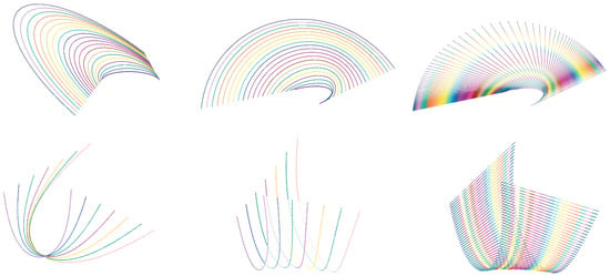
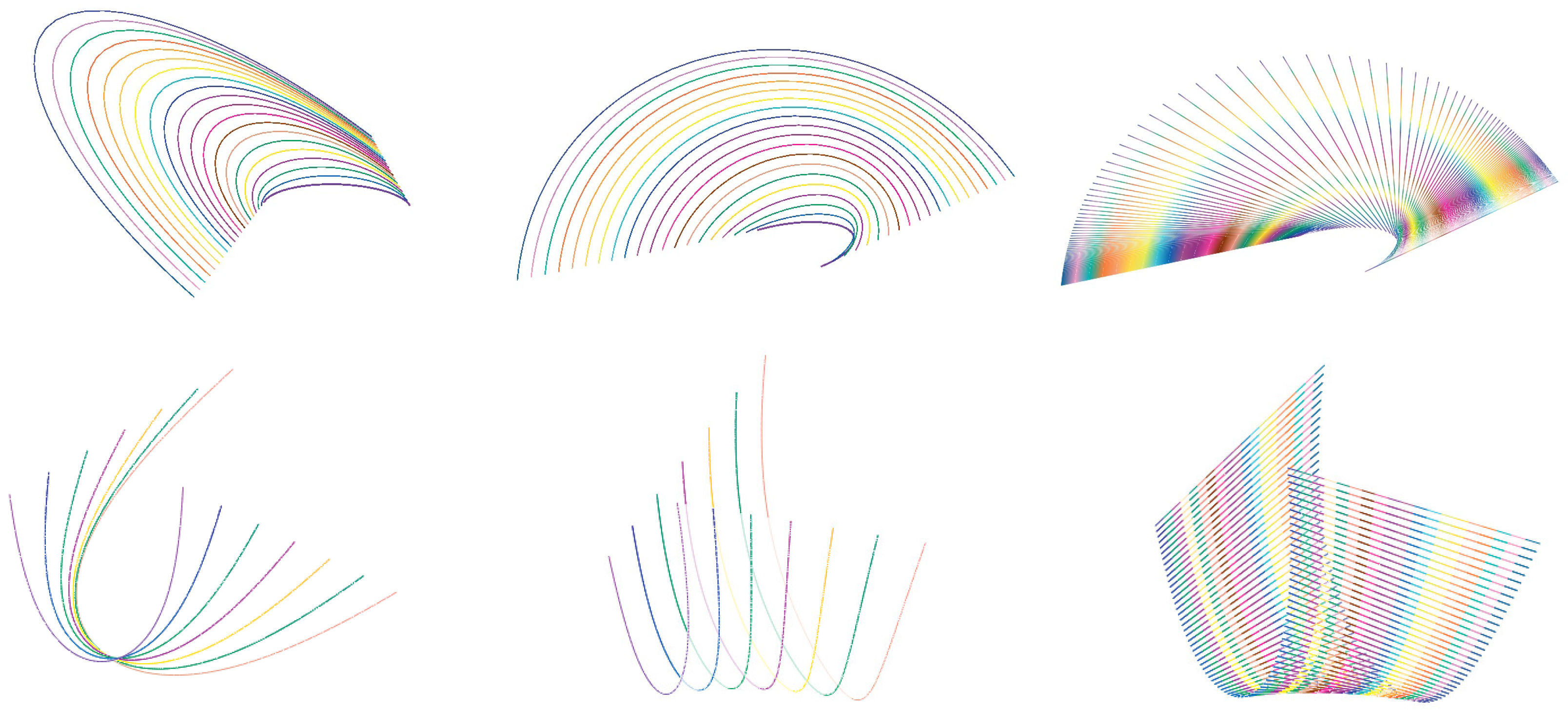
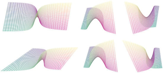
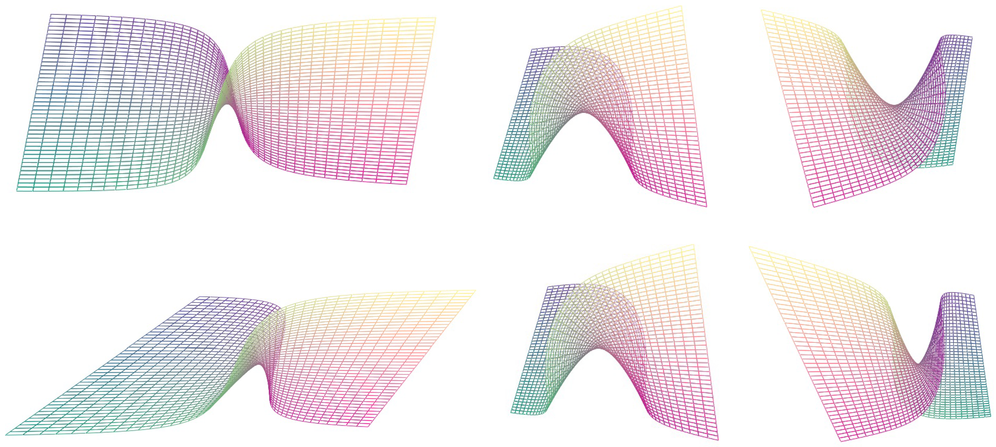
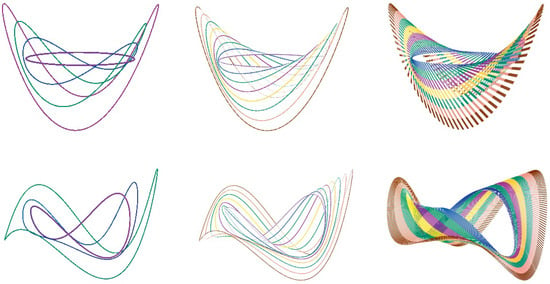
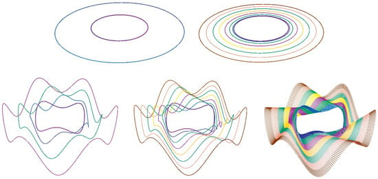
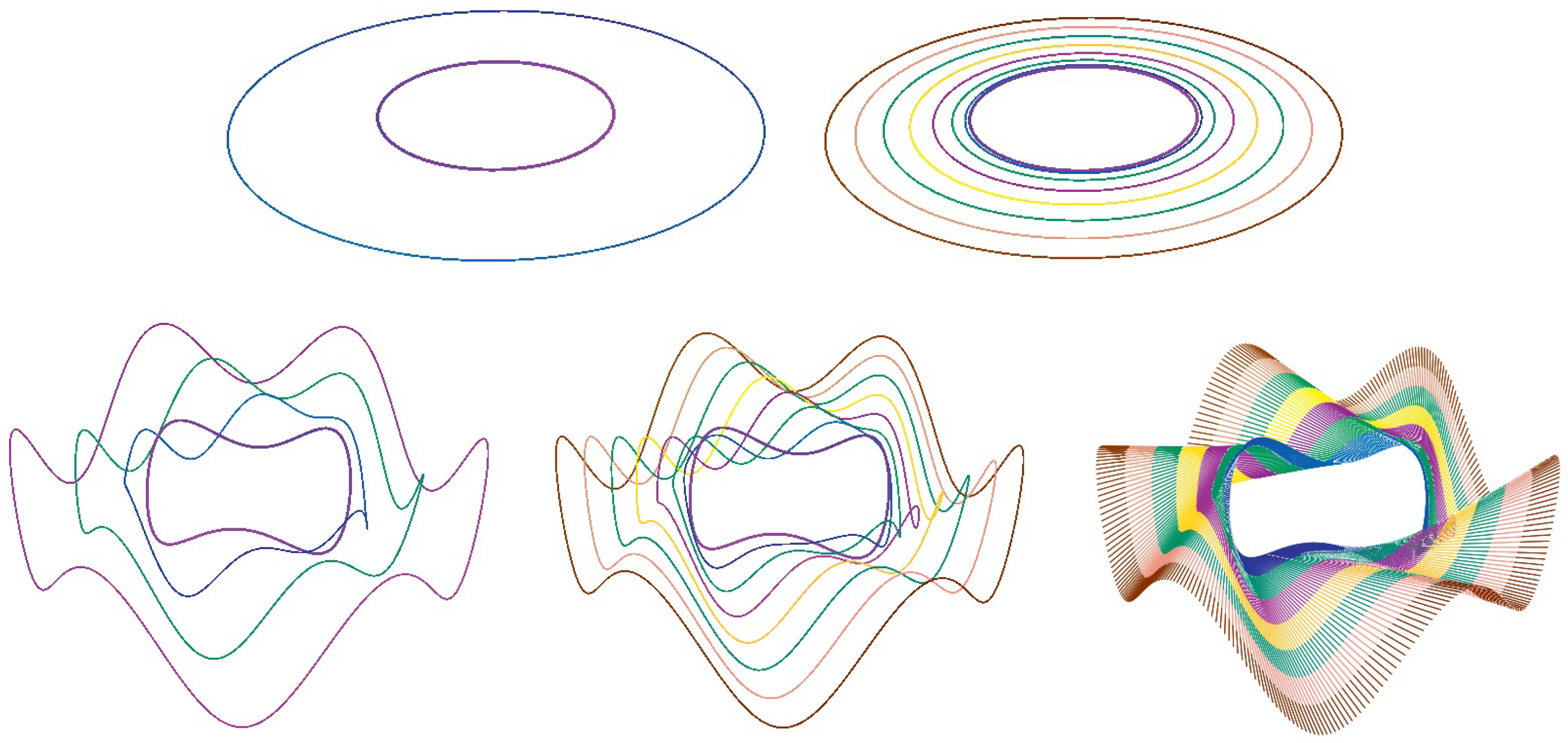
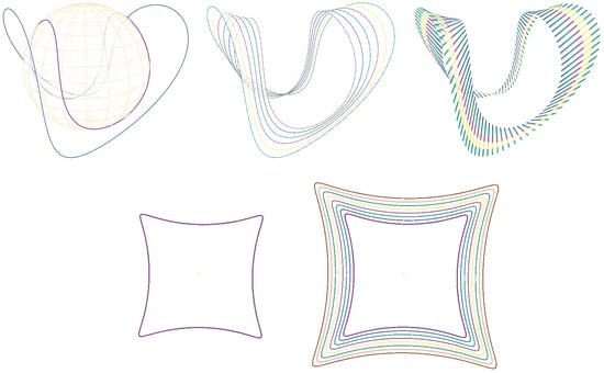
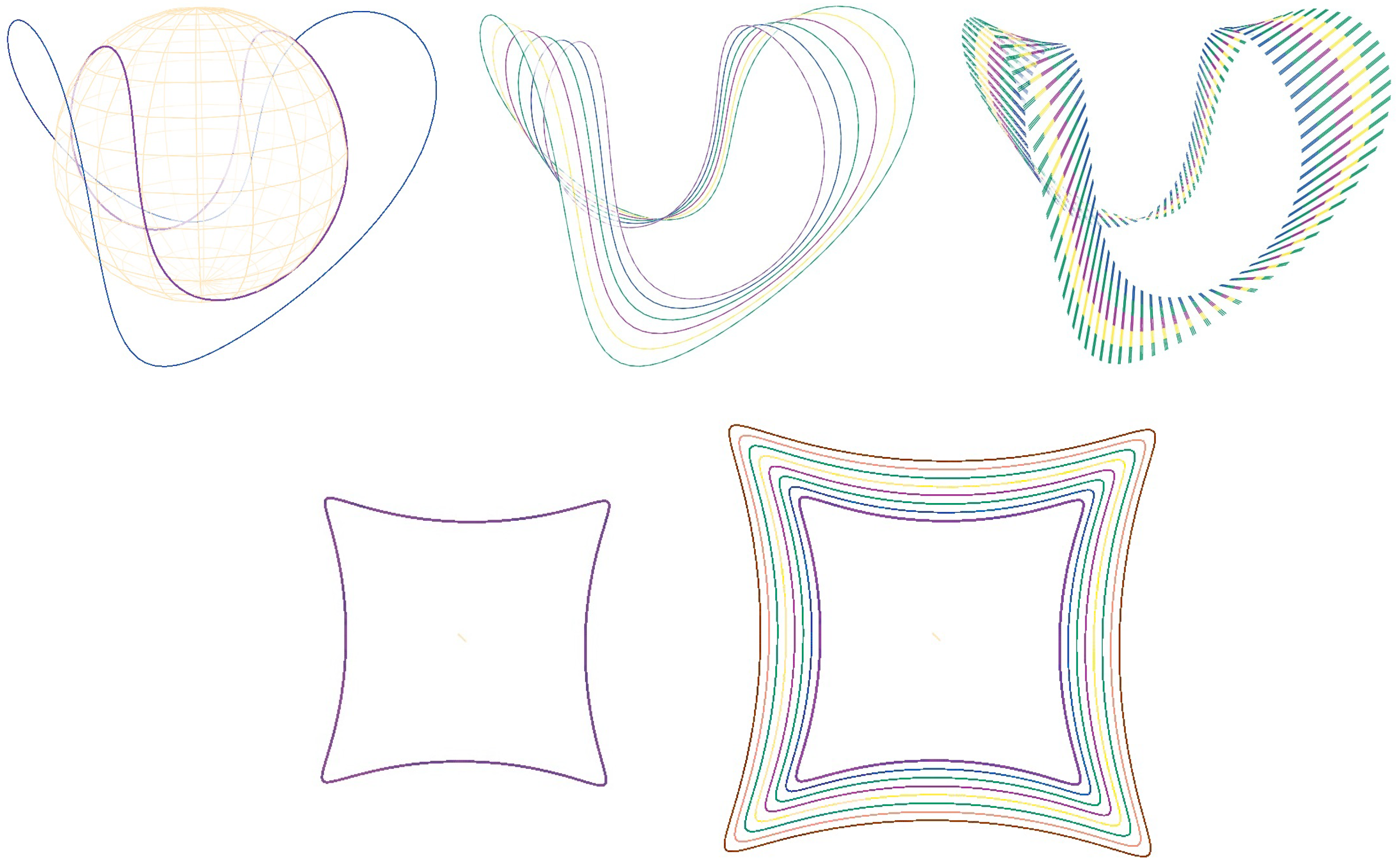
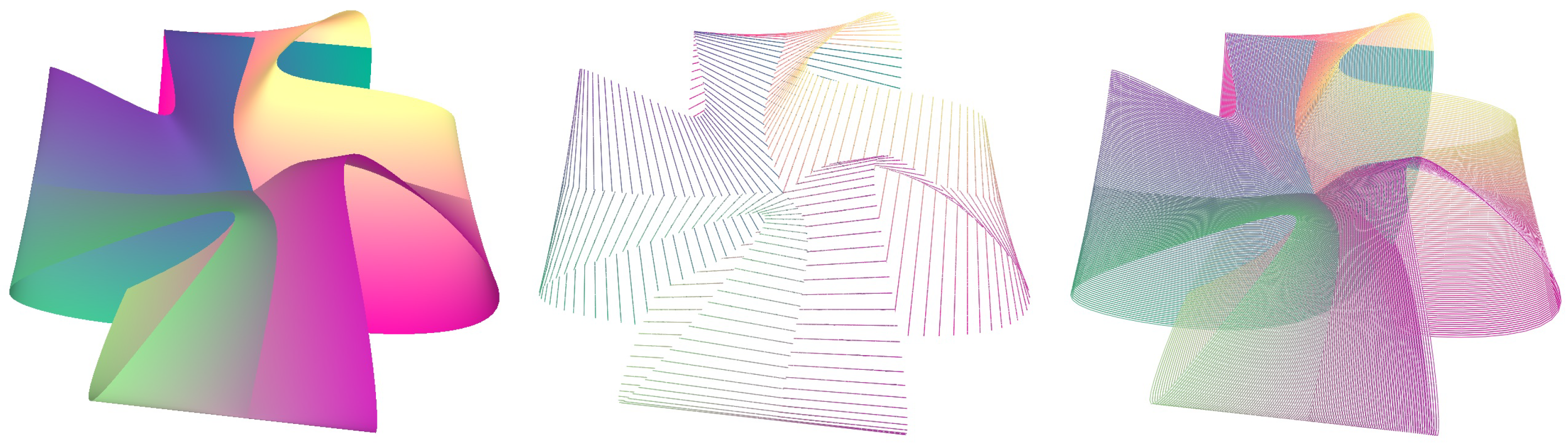
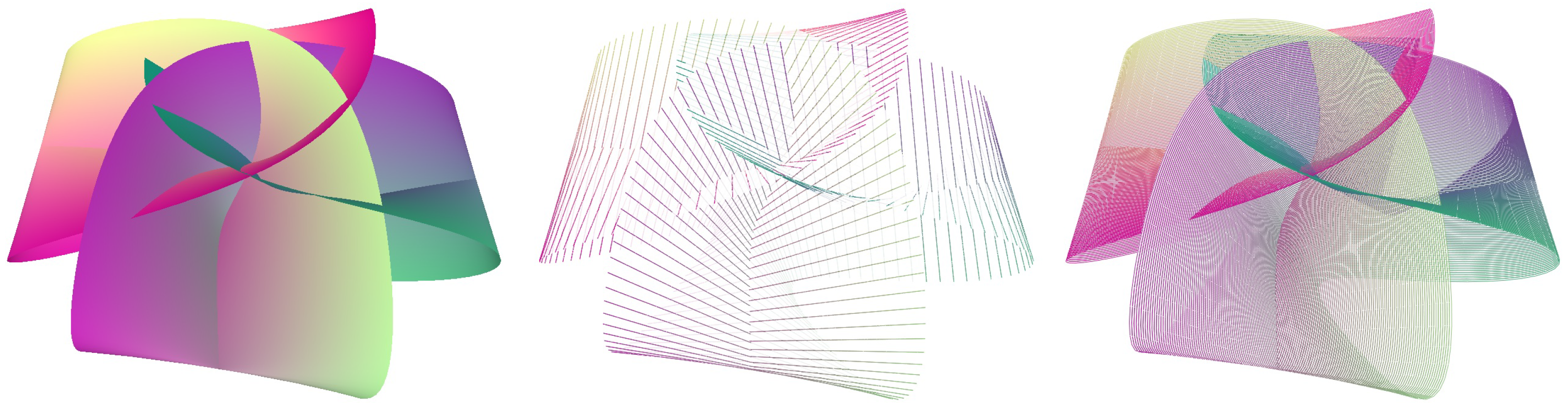
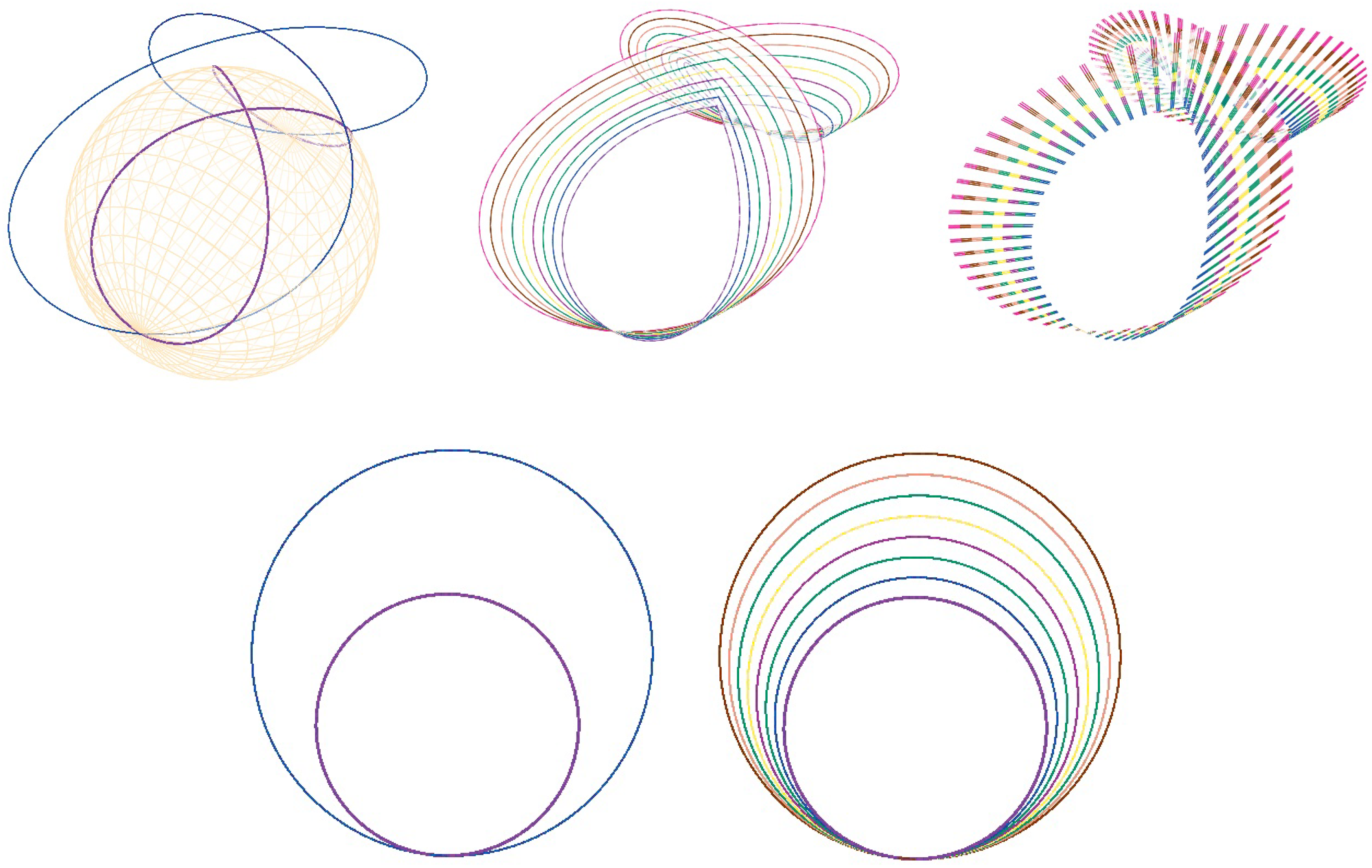
In the following examples, we will show what happens to the indicatrix $C: \mathbf{r}=\mathbf{r}\left(u\right)$ and the dual part $C^{*}: {\mathbf{r}}^{*}={\mathbf{r}}^{*}\left(u\right)$ of the dual curve during infinitesimal bending, as well as to the corresponding ruled surface under the action of the dual bending field (see Figure 1, Figure 2, Figure 3, Figure 4, Figure 5, Figure 6, Figure 7, Figure 8, Figure 9, Figure 10 and Figure 11).

Figure 1. Family of indicatrices (up) and dual parts (down) under the infinitesimal bending of the dual curve ${\tilde{C}}_1$.

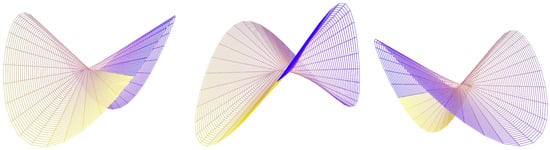
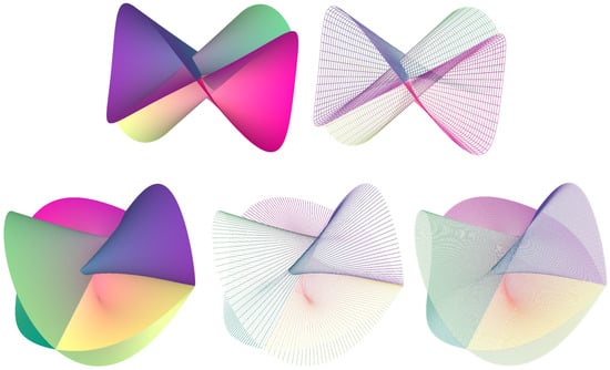
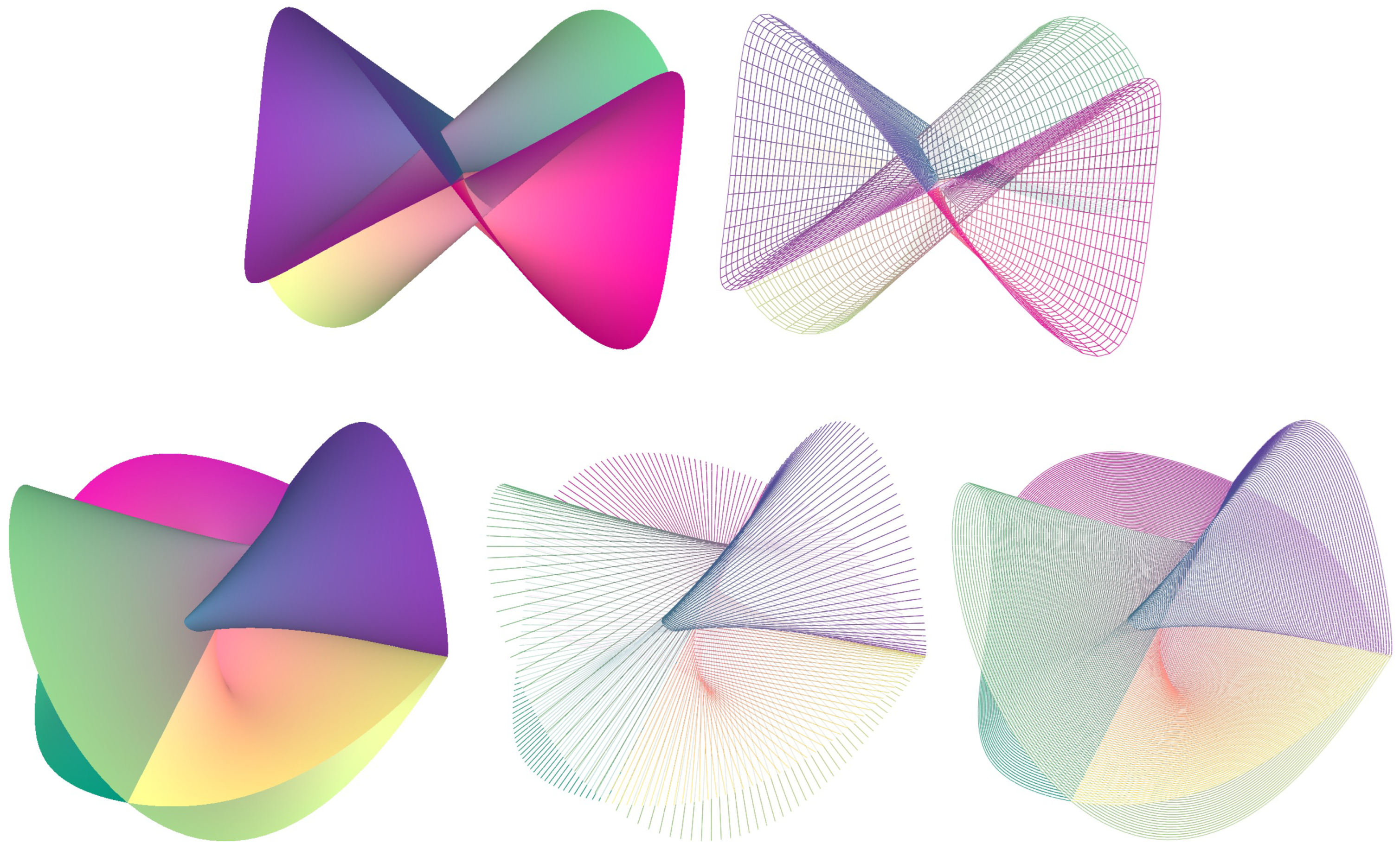
Figure 2. Deformed surfaces corresponding to the dual curve ${\tilde{C}}_{1t}$ for $t=0.03$ (up) and for $t=0.25$ (down) (different points of view).

Figure 3. Family of indicatrices (up) and dual parts (down) under the infinitesimal bending of the dual curve ${\tilde{C}}_2$.

Figure 4. Deformed surface corresponding to the dual curve ${\tilde{C}}_{2t}$ for $t=0.1$ (different points of view).

Figure 5. Family of indicatrices (up) and dual parts (down) under the infinitesimal bending of the dual curve ${\tilde{C}}_3$.

Figure 6. Deformed surface corresponding to the dual curve ${\tilde{C}}_{3t}$ for $t=0.1$ (different points of view).

Figure 7. Family of indicatrices (up) and dual parts (down) under the infinitesimal bending of the dual curve ${\tilde{C}}_4$.

Figure 8. Deformed surface corresponding to the dual curve ${\tilde{C}}_{4t}$ for $t=0.1$ (view on one side).

Figure 9. Deformed surface corresponding to the dual curve ${\tilde{C}}_{4t}$ for $t=0.1$ (view on the other side).

Figure 10. Family of indicatrices (up) and dual parts (down) under the infinitesimal bending of the dual curve ${\tilde{C}}_5$.

Figure 11. Deformed surface corresponding to the dual curve ${\tilde{C}}_{5t}$ for $t=0.1$ from different points of view.

It is interesting to note that the infinitesimal bending of a real curve of parameter u determines a surface with two parameters: one is the curve parameter u and the other is the bending parameter t. Surfaces generated by infinitesimal bending of a real curve were considered in [25,26]. Here, we will provide a visual representation of the two surfaces that are obtained during the infinitesimal bending of a dual curve, one consisting of the family of curves resulting from the deformation of the indicatrix, and the other of the family of curves resulting from the deformation of the dual part of the corresponding dual curve (see the third pictures in Figure 1, Figure 3, Figure 5, Figure 7 and Figure 10).

All figures are displayed using our own software tool written in Microsoft Visual C++ (VS 2022). The 3D modeling and visualization with semitransparent objects were carried out in OpenGL (1.5).

The examples presented in this section serve to illustrate different types of dual infinitesimal bending fields, considering sphere-preserving cases, and to visualize the corresponding deformations of ruled surfaces. The dual bending fields used in the examples were chosen to satisfy the conditions of Theorems 1 and 5. While the examples are not intended as a classification, they demonstrate the applicability of the theoretical results and the qualitative behavior of the induced deformations.

Example 1.

Let us consider the dual curve ${\tilde{C}}_1: \tilde{\mathbf{r}}=\tilde{\mathbf{r}}\left(u\right)$ on the dual unit sphere ${\mathbb{S}}^2$, determined by

$$\tilde{\mathbf{r}}\left(u\right)=\mathbf{r}\left(u\right)+ϵ{\mathbf{r}}^{*}\left(u\right)={\displaystyle \frac{1}{\sqrt{2+4u^2}}}(1,-1,2u)+{\displaystyle \frac{ϵ}{\sqrt{2+4u^2}}}(u^2,-u^2,-u).$$

(50)

This dual curve represents the hyperbolic paraboloid (see [17]). The corresponding dual bending field is

$$\tilde{\mathbf{z}}\left(u\right)=\mathbf{z}\left(u\right)+ϵ{\mathbf{z}}^{*}\left(u\right)={\displaystyle \frac{1}{\sqrt{2+4u^2}}}(-2u-1,2u-1,2)+{\displaystyle \frac{ϵ}{\sqrt{2+4u^2}}}(u-1,-u-1,2u^2)$$

(51)

and it determines the family of indicatrices (Figure 1, up)

$$C_{1t}: {\mathbf{r}}_t\left(u\right)={\displaystyle \frac{1}{\sqrt{2+4u^2}}}(1,-1,2u)+{\displaystyle \frac{t}{\sqrt{2+4u^2}}}(-2u-1,2u-1,2)$$

(52)

and the family of dual parts (Figure 1, down)

$$C_{1t}^{*}: {\mathbf{r}}_t^{*}\left(u\right)={\displaystyle \frac{1}{\sqrt{2+4u^2}}}(u^2,-u^2,-u)+{\displaystyle \frac{t}{\sqrt{2+4u^2}}}(u-1,-u-1,2u^2).$$

(53)

A direct computation shows

$$\dot{\mathbf{r}}\left(u\right)={\displaystyle \frac{4}{{(2+4u^2)}^{3/2}}}(-u,u,1), {\dot{\mathbf{r}}}^{*}\left(u\right)={\displaystyle \frac{2}{{(2+4u^2)}^{3/2}}}(2u^3+2u,-2u^3-2u,-1),$$

$$\dot{\mathbf{z}}\left(u\right)={\displaystyle \frac{4}{{(2+4u^2)}^{3/2}}}(u-1,u+1,-2u),$$

$${\dot{\mathbf{z}}}^{*}\left(u\right)={\displaystyle \frac{2}{{(2+4u^2)}^{3/2}}}(2u+1,2u-1,4u^3+4u),$$

$$\mathbf{r}\left(u\right)·\mathbf{z}\left(u\right)=0 \wedge {\mathbf{r}}^{*}\left(u\right)·\mathbf{z}\left(u\right)+\mathbf{r}\left(u\right)·{\mathbf{z}}^{*}\left(u\right)=0,$$

$$\dot{\mathbf{r}}\left(u\right)·\dot{\mathbf{z}}\left(u\right)=0 \wedge {\dot{\mathbf{r}}}^{*}\left(u\right)·\dot{\mathbf{z}}\left(u\right)+\dot{\mathbf{r}}\left(u\right)·{\dot{\mathbf{z}}}^{*}\left(u\right)=0,$$

confirming that it represents a sphere-preserving infinitesimal bending field in accordance with Theorems 1 and 5. The family of ruled surfaces is given by Equation (49), and the corresponding surfaces for $t=0.03$ and $t=0.25$ are given in Figure 2.

Example 2.

The dual spherical curve ${\tilde{C}}_2: \tilde{\mathbf{r}}\left(u\right)=\mathbf{r}\left(u\right)+ϵ{\mathbf{r}}^{*}\left(u\right)$ where

$$C_2: \mathbf{r}\left(u\right)=(cosu,sinu,0), C_2^{*}:{\mathbf{r}}^{*}\left(u\right)=(sinu,-cosu,0),$$

(54)

is deformed by the dual vector field $\tilde{\mathbf{z}}\left(u\right)=\mathbf{z}\left(u\right)+ϵ{\mathbf{z}}^{*}\left(u\right)$,

$$\mathbf{z}\left(u\right)=(-sinu,cosu,sinu), {\mathbf{z}}^{*}\left(u\right)=(cosu,sinu,cosu).$$

(55)

The family ${\tilde{C}}_{2t}$ is the dual infinitesimal bending on the dual sphere with a given precision. The graphic illustration of the family of indicatrices, as well as of the dual parts, is given in Figure 3. The corresponding deformed surface for $t=0.1$ is given in Figure 4.

Example 3.

The dual spherical curve ${\tilde{C}}_3: \tilde{\mathbf{r}}\left(u\right)=\mathbf{r}\left(u\right)+ϵ{\mathbf{r}}^{*}\left(u\right)$ where

$$C_3: \mathbf{r}\left(u\right)=(cosu,sinu,0), C_3^{*}:{\mathbf{r}}^{*}\left(u\right)=(sinu,-cosu,0.3sin3u),$$

(56)

is deformed by the dual vector field $\tilde{\mathbf{z}}\left(u\right)=\mathbf{z}\left(u\right)+ϵ{\mathbf{z}}^{*}\left(u\right)$,

$$\mathbf{z}\left(u\right)=(-sinu,cosu,0), {\mathbf{z}}^{*}\left(u\right)=(cosu,sinu,0.3cos6u).$$

(57)

The family ${\tilde{C}}_{3t}$ is the dual infinitesimal bending on the dual sphere with a given precision. The graphic illustration of the family of indicatrices, as well as of the dual parts, is given in Figure 5. The corresponding deformed surface for $t=0.1$ is given in Figure 6.

Example 4.

The seam line of a tennis ball curve ${\tilde{C}}_4: \tilde{\mathbf{r}}\left(u\right)=\mathbf{r}\left(u\right)+ϵ{\mathbf{r}}^{*}\left(u\right)$ where

$$C_4: \mathbf{r}\left(u\right)=(acosu+bcos3u,a sinu-bsin3u,csin2u),$$

(58)

$$C_4^{*}:{\mathbf{r}}^{*}\left(u\right)=(acosu+bcos3u,a sinu-bsin3u,1.8cos2u).$$

(59)

For $a=0.8$, $b=0.2$ and $c=0.8$, it is deformed by the dual vector field $\tilde{\mathbf{z}}\left(u\right)=\mathbf{z}\left(u\right)+ϵ{\mathbf{z}}^{*}\left(u\right)$,

$$\mathbf{z}\left(u\right)=(asinu-bsin3u,-acosu-bcos3u,0),$$

(60)

$${\mathbf{z}}^{*}\left(u\right)=(asinu-bsin3u,-acosu-bcos3u,0).$$

(61)

The family ${\tilde{C}}_{4t}$ is the dual infinitesimal bending on the dual sphere with a given precision. The graphic illustration of the family of indicatrices, as well as of the dual parts, is given in Figure 7. The corresponding deformed surface for $t=0.1$ is given in Figure 8 and Figure 9.

Example 5.

The Viviani curve ${\tilde{C}}_5: \tilde{\mathbf{r}}\left(u\right)=\mathbf{r}\left(u\right)+ϵ{\mathbf{r}}^{*}\left(u\right)$ where

$$C_5: \mathbf{r}\left(u\right)=(a{cos}^{2}u,a cosusinu,a sinu),$$

(62)

$$C_5^{*}:{\mathbf{r}}^{*}\left(u\right)=(a{cos}^{2}u,a cosusinu,3sinu).$$

(63)

For $a=4$, it is deformed by the dual vector field $\tilde{\mathbf{z}}\left(u\right)=\mathbf{z}\left(u\right)+ϵ{\mathbf{z}}^{*}\left(u\right)$,

$$\mathbf{z}\left(u\right)=(acosusinu,-a{cos}^{2}u,0),$$

(64)

$${\mathbf{z}}^{*}\left(u\right)=(acosusinu,-a{cos}^{2}u,0).$$

(65)

The family ${\tilde{C}}_{5t}$ is the dual infinitesimal bending on the dual sphere with a given precision. The graphic illustration of the family of indicatrices, as well as of the dual parts, is given in Figure 10. The corresponding deformed surface for $t=0.1$ is given in Figure 11.

6. Conclusions

The problem of the infinitesimal bending of dual curves first occurs in [16]. According to the theory of the infinitesimal bending of curves and surfaces in Euclidean 3-space ${\mathbb{R}}^3$, the basic idea is to infinitesimally deform dual curves in the dual 3-space ${\mathbb{D}}^3$ such that the dual arc length is invariant with a predetermined precision. This paper presents the continuation of the authors’ research on this topic. The paper provides new characterizations of the infinitesimal bending of a dual curve with the necessary and sufficient conditions for the dual bending field and explicitly determined formulas. In particular, dual spherical curves, which correspond to the ruled surfaces according to E. Study’s mapping, are considered. Finally, examples of the infinitesimal bending of dual curves with specific dual fields are given, together with a graphical representation.

From a geometric point of view, the obtained conditions describe admissible infinitesimal deformations of dual curves and the associated ruled surfaces that preserve dual arc length and, in the spherical case, the dual unit sphere. This provides insight into the infinitesimal flexibility and rigidity of ruled surfaces represented in the dual setting and clarifies the role of dual geometric invariants in controlling such deformations.

In addition to contributing to the theory of dual curves, this paper proposes new questions: What happens with geometric quantities describing the dual curve? How does its shape change? How do special classes of dual curves behave under infinitesimal bending? How do the infinitesimal rigidity and flexibility of specific classes of ruled surfaces depend on the geometric invariants of the associated dual curves? These and similar questions will be the subject of future research.

References

- Study, E. Geometrie der Dynamen; Druck und verlag von b. g. Teubner: Leipzig, Germany, 1903. [Google Scholar]
- Bottema, O.; Roth, B. Theoretical Kinematics; North-Holland Publishing Company: Amsterdam, The Netherlands, 1979. [Google Scholar]
- Pottman, H.; Wallner, J. Computational Line Geometry; Springer: Berlin/Heidelberg, Germany, 2001. [Google Scholar]
- Abdel-Baky, R.; Saad, M.K. Some characterizations of dual curves in dual 3-space D3. AIMS Math. 2021, 6, 3339–3351. [Google Scholar] [CrossRef] [Scilit]
- Li, Y.; Pei, D. Evolutes of dual spherical curves for ruled surfaces. Math. Meth. Appl. Sci. 2016, 39, 3005–3015. [Google Scholar] [CrossRef] [Scilit]
- Mazlum, S.G.; Şenyurt, S.; Grilli, L. The Invariant of Dual Parallel Equidistant Ruled Surfaces. Symmetry 2023, 15, 206. [Google Scholar] [CrossRef] [Scilit]
- Önder, M.; Uǧurlu, H.H. Normal and Spherical Curves in Dual Space D3. Mediterr. J. Math. 2013, 10, 1527–1537. [Google Scholar] [CrossRef] [Scilit]
- Yücesan, A.; Tükel, G.Ö. Dual Spherical Elastica. Filomat 2023, 37, 2483–2493. [Google Scholar] [CrossRef] [Scilit]
- Belova, O.; Mikeš, J.; Sherkuziyev, M. An Analytical Inflexibility of Surfaces Attached Along a Curve to a Surface Regarding a Point and Plane. Results Math. 2021, 76, 56. [Google Scholar] [CrossRef] [Scilit]
- Broscăteanu, Ş.-C.; Mihai, A.; Olteanu, A. A note on the Infinitesimal Bending of a Rectifying Curve. Symmetry 2024, 16, 1361. [Google Scholar] [CrossRef] [Scilit]
- Efimov, N.V. Qualitative problems of the theory of deformation of surfaces. Uspekhi Mat. Nauk 1948, 3, 47–158. [Google Scholar]
- Kon-Fossen, S.E. Nekotorye Voprosy Differencial’noj Geometrii v Celom; Gosudarstvennoe Izdatel’stvo Fiziko-Matematicheskoj Literatury: Moscow, Russia, 1959. [Google Scholar]
- Vekua, I.N. Obobscchennye Analiticheskie Funkcii; Nauka: Moscow, Russia, 1988; pp. 305–434. [Google Scholar]
- Najdanović, M.S.; Rančić, S.R.; Velimirović, L.S. Total Torsion and Spherical Curves Bending. Mediterr. J. Math. 2024, 21, 74. [Google Scholar] [CrossRef] [Scilit]
- Velimirović, L.S.; Jamali, M.; Shahid, M.H.; Najdanović, M.S.; Rančić, S.R. Willmore energy and total normalcy of knots. Filomat 2025, 39, 2655–2667. [Google Scholar] [CrossRef] [Scilit]
- Najdanović, M.S. Characterization of dual curves using the theory of infinitesimal bending. Math. Meth. Appl. Sci. 2024, 47, 8626–8637. [Google Scholar] [CrossRef] [Scilit]
- Najdanović, M.S.; Velimirović, L.S.; Rančić, R.S. Deformations preserving dual arc length in dual 3-space. Facta Univ. Ser. Math. Inform. 2024, 39, 891–897. [Google Scholar] [CrossRef] [Scilit]
- Durmaz, O.; Aktaş, B.; Gündoğan, H. New approaches on dual space. Facta Univ. 2020, 35, 437–458. [Google Scholar] [CrossRef] [Scilit]
- Guggenheimer, H.W. Differential Geometry; Dover Publications, Inc.: New York, NY, USA, 1977; pp. 162–168. [Google Scholar]
- Veldkamp, G.R. On the Use of Dual Numbers, Vectors and Matrices in Instantaneous, Spatial Kinematics. Mech. Mach. Theory 1974, 11, 141–156. [Google Scholar] [CrossRef] [Scilit]
- Durmaz, O.; Aktaş, B.; Keçilioğlu, O. An overview to analyticity of dual functions. Commun. Fac. Sci. Univ. Ank. Ser. A1 Math. Stat. 2022, 71, 1095–1120. [Google Scholar] [CrossRef] [Scilit]
- Messelmi, F. Analysis of Dual Functions. Annu. Rev. Chaos Theory Bifurcations Dyn. Syst. 2013, 4, 37–54. [Google Scholar]
- Abdel Baky, R.A. An explicit characterization of dual spherical curve. Commun. Fac. Sci. Univ. Ank. Ser. A1 2002, 51, 1–9. [Google Scholar]
- Gray, A. Modern Differential Geometry of Curves and Surfaces with Mathematica; CRC Press: Boca Raton, FL, USA, 1998; p. 231. [Google Scholar]
- Gözütok, Ü.; Çoban, H.A.; Saǧiroģlu, Y. Ruled surfaces obtained by bending of curves. Turk. J. Math. 2020, 44, 300–306. [Google Scholar] [CrossRef] [Scilit]
- Rančić, S.; Najdanović, M.; Velimirović, L. Surfaces defined by bending of knots. Filomat 2019, 37, 8635–8640. [Google Scholar] [CrossRef] [Scilit]
Disclaimer/Publisher’s Note: The statements, opinions and data contained in all publications are solely those of the individual author(s) and contributor(s) and not of MDPI and/or the editor(s). MDPI and/or the editor(s) disclaim responsibility for any injury to people or property resulting from any ideas, methods, instructions or products referred to in the content. |
© 2026 by the authors. Licensee MDPI, Basel, Switzerland. This article is an open access article distributed under the terms and conditions of the Creative Commons Attribution (CC BY) license.