Abstract
Differential equations have demonstrated significant practical effectiveness across diverse fields, including physics, chemistry, biological engineering, computer science, electrical power systems, and security cryptography. This study investigates the dynamics of a Caputo fractional discrete-time modified Brusselator model. Conditions for the existence and local stability of the fixed point are established. Using bifurcation theory, the occurrence of both period-doubling and Neimark–-Sacker bifurcations is analyzed, revealing that these bifurcations occur at specific values of the bifurcation parameter. Maximum Lyapunov characteristic exponents are computed to assess system sensitivity. Two-dimensional diagrams are presented to illustrate phase portraits, local stability regions, closed invariant curves, bifurcation types, and Lyapunov exponents, while the 0-1 test confirms the presence of chaos in the model. Finally, MATLAB simulations validate the theoretical results.
Keywords:
chemical reaction; Caputo fractional derivative; discretization; stability analysis; bifurcations; 0-1 test; chaos MSC:
39A30; 40A05; 92D25; 92C50
1. Introduction
Formulating appropriate differential equations to analyze the dynamics of chemical reactions is a fundamental task in applied sciences. A chemical reaction refers to the transformation of one or more substances into different compounds, and such processes are encountered in numerous contexts, ranging from natural ecosystems to industrial production. Classical examples include combustion, the smelting of metals, fuel burning, and glass and ceramic manufacturing, as well as food processing. In biological systems, photosynthesis in plants converts carbon dioxide and water into glucose and oxygen, while, in the human body, enzymatic reactions ensure vital functions such as digestion. For instance, the enzyme amylase is responsible for initiating the decomposition of complex sugars into simpler units. Electrochemical reactions, on the other hand, serve as the basis for modern batteries, allowing chemical energy to be transformed into electrical power.
The study of these processes increasingly relies on mathematical tools. Nonlinear dynamical features, such as equilibrium stability, oscillatory patterns, bifurcations, chaos, and boundedness, are frequently observed in chemical systems. By applying mathematical modeling, one can not only interpret experimental outcomes, but also predict new behaviors and interactions between chemical variables. Among modern approaches, fractional-order differential equations have proven to be especially effective at capturing the intricate dynamics and memory effects present in chemical reaction systems. Several studies have addressed these dynamics. Asheghi [1] examined diffusion effects and Hopf bifurcation in a reduced Gierer–Meinhardt model, while Chen and Wang [2] analyzed boundedness and Hopf bifurcation in a generalized Lengyel–Epstein system. Wong and Ward [3] developed a hybrid asymptotic–numerical approach for spot patterns in the Schnakenberg model. Xu et al. [4] studied existence, stability, and Hopf bifurcation in a fractional delayed Brusselator model, and later in [5] investigated the fractional delayed Oregonator system, showing delay-driven stability changes. Din [6] considered a three-dimensional chaotic system and proved global stability using a Lyapunov function, while in [7] the same author explored discretization, bifurcations, and chaos control in the Schnakenberg model. Kol’tsov [8] analyzed chaotic oscillations in a three-intermediate reaction system. Monwanou et al. [9] studied a four-molecule system, presenting bifurcations, Lyapunov exponents, and phase portraits. Bodale and Oancea [10] investigated chaos control in the Willamowski–Rössler model, and Binous [11] reported on several chemical engineering problems involving limit cycles, chaos, and Hopf bifurcations. Moreover, the Noyes–Field model of the time-fractional Belousov–Zhabotinsky reaction system was analyzed analytically in [12] utilizing the natural transform decomposition approach. Chi [13] investigated the chemo-mechanical model while Karimov et al. [14] used a unique 8-cell photometer technique to examine the process of action in a stirring-controlled Belousov–Zhabotinsky interaction.
Nonlinear reaction–diffusion systems, particularly the Brusselator model, are frequently employed for explaining complex chemical and biological processes. These systems can display a variety of dynamical behaviors, including as oscillations, pattern creation, and chaos. Although classical integer-order models have been extensively investigated, new discoveries emphasize the importance of fractional-order differential equations, particularly in the Caputo sense, for capturing features of such systems. Fractional-order models, in particular, can provide more accurate and adaptable structures for modeling chemical kinetics and biological interactions across time. This research is motivated by the desire to better understand how fractional-order dynamics affect the stability and chaotic behavior of a modified Brusselator model. The main contribution of this paper is embedded in providing a comprehensive examination of dynamical systems, including fixed points, bifurcations, and chaotic transitions. Moreover, this study implements and verifies the 0-1 test as an effective instrument to identify chaos in complex fractional-order systems. This research not only expands the theoretical knowledge of fractional nonlinear dynamical systems, but it additionally offers practical tools and insights for researchers in chemical kinetics, biological modeling, and control theory.
This manuscript is designed as follows. Section 2 presents the description of the used model while Section 3 highlights the discretization process of our model using the Caputo fractional derivative. In Section 4, we analyze the local stability of the fixed points while we investigate the period-doubling bifurcation in Section 5. Furthermore, the Neimark–Sacker bifurcation is given in Section 6 and the chaos control is examined in Section 7. Section 8 is devoted to demonstrate some numerical simulations. In Section 9, the 0-1 test for chaos is applied to distinguish between regular and chaotic dynamics of the system. Section 10 discusses the most important outcomes, and Section 11 concludes this paper.
2. Model Description
This part shows how to develop the Brusselator model. The oscillatory behavior observed in the Brusselator reaction is similar to that of the Belousov–Zhabotinsky reaction. According to [15], the Brusselator is a theoretical model of an oscillating chemical reaction. Moreover, it represents a minimal mathematical system which is capable of exhibiting oscillatory behavior. The Brusselator reaction can be generally described by the following sequence of chemical steps:
where and represent chemical reactants or products. Furthermore, the schematic diagram of the chemical reaction system in (1) is illustrated in Figure 1. In [16], Chen investigated the following Brusselator model:
Moreover, the dimensionless form of System (2) is given by [16,17]:
where , and both and are positive and proportional to the concentrations of the reactants and , respectively. The nonlinear term describes the autocatalytic step. Consequently, if we assume that the autocatalytic step occurs over a shorter timescale, we can modify the term by introducing a new non-linear restraint term, which is . Replacing the term in Model (3) by the term leads to the following modified Brusselator model:
Here, the chemical motivation for the term is to represent nonlinear saturation effects typically seen in practical autocatalytic reactions. This modification allows the model to have substrate inhibition when B is massive, while maintaining normal Brusselator behavior if B is small. According to [18], chaos is characterized by three essential properties, namely, long-term aperiodic behavior, determinism, and sensitive dependence on initial conditions. This implies that nearby trajectories diverge exponentially, which is associated with a positive Lyapunov exponent. In continuous systems with a two-dimensional phase space, such an exponential divergence cannot occur. Consequently, chaotic behavior is only possible in deterministic continuous systems with a phase space of at least three dimensions. Therefore, chaotic dynamics are not possible in the continuous version of System (4). Considering that fractional calculus enables a more accurate modeling of complex systems that cannot be effectively described by integer-order differential equations and that fractional-order systems can be flexibly adapted to fit a wide range of data sets, it is therefore more appropriate to study the fractional-order counterpart of System (4).
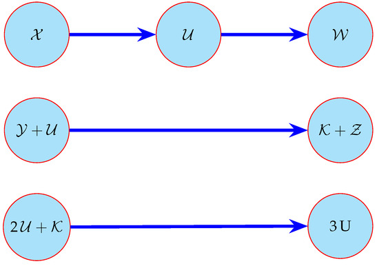
Figure 1.
Diagram for the chemical reaction in (1).
The motivation for this study arises from several considerations. First, there is a noticeable gap in the literature on the detailed analysis of bifurcation types in chemical reaction models. Second, fractional differential equations offer a powerful framework for investigating the complex dynamics of chemical systems. The primary objective of this work is to analyze the fixed point, assess its local stability, and explore the occurrence of period-doubling and Neimark–Sacker bifurcations in the following fractional-time-modified Brusselator model:
where is the fractional-order parameter, and denotes the Caputo fractional derivative, which is defined as follows.
Definition 1.
The Caputo fractional derivative of order of a function is defined as follows:
where is the Gamma function and κ is the fractional order.
3. Discretization Process Using the Caputo Fractional Derivative
The Caputo fractional derivative is a valuable mathematical instrument for modeling dynamic systems with memory and hereditary features. Unlike classical integer-order derivatives, it takes into consideration the history of a system’s previous states, making it particularly efficient at capturing complicated practical behaviors. One of its primary benefits is its ability to comply with initial conditions described in terms of integer-order derivatives, which is common in both chemical and physical phenomena. The purpose of this section is to discretize the fractional-time Model (5), employing the piecewise constant argument strategy, as outlined in [19,20,21]. We begin with the following system:
Here, represents the step size.
- Step 1: For , we have . Thus, the system becomesSystem (6) is simplified to
- Step 2: For , we have . Then, the system becomesThe solution to this system is
- Step 3: For , we have . The system is given byThe solution to this system is given by
- Generalization: After n iterations, the system can be written aswhere for .
- Final Discretized System: As , the discretized version of System (5) becomes
4. Local Stability of the Fixed Point of System (7)
In this section, we examine the existence of a positive fixed point for the discrete chemical reaction system in (7). Additionally, we provide a thorough analysis of the local stability of this positive fixed point. To determine the fixed points of System (7), we solve the following algebraic system:
Thus, we obtain the following system of equations for the fixed points:
Hence, the unique positive fixed point is denoted as . Next, we analyze the stability of the fixed point with the help of the following definition and lemma [19,22,23].
Definition 2
([24,25,26]). The following situations are valid for the equilibrium point of any system:
- 1.
- If and , it is a sink point and locally asymptotically stable;
- 2.
- If and , it is a source point and locally unstable;
- 3.
- If and or ( and ), it is a saddle point;
- 4.
- If or , it is non-hyperbolic.
Lemma 1
([24,25,26]). Let us consider such that . In addition, and are the two roots of . Then, the following hold:
- 1.
- and if and only if and .
- 2.
- and if and only if and .
- 3.
- and (or and ) if and only if .
- 4.
- and if and only if and .
- 5.
- and are complex numbers and if and only if and .
The Jacobian matrix evaluated at the fixed point (A,B), corresponding to the linearization of System (7), is given by
Lemma 2.
For the unique positive fixed point of System (7), the following statements are true:
- 1.
- If any one of the following conditions holds, then is locally asymptotically stable (i.e., a sink):
- i
- and
- ii
- and
- 2.
- If any one of the following conditions holds, then is unstable (i.e., a source):
- i
- and
- ii
- and
- 3.
- The fixed point is unstable (i.e., a saddle point) if
- 4.
- The fixed point is non-hyperbolic if one of the following conditions holds:
- i
- and
- ii
- and and
Proof.
The Jacobian matrix (10) at is defined as
The characteristic polynomial associated with the Jacobian matrix at the fixed point is given by
where
To further analyze the stability, we evaluate the characteristic polynomial at specific values of ℘, as follows:
and the discriminant of Polynomial (12) is given by
Since , by invoking Definition 2 and Lemma 1, we obtain the results of Lemma 2.
- This completes the proof. □
Theorem 1.
The unique positive fixed point of System (7) loses its stability as follows:
- i
- Via a period-doubling bifurcation if
- ii
- Via a Neimark–Sacker bifurcation if
Proof.
As discussed in [19,23,27,28] and shown through Lemma 2, a period-doubling bifurcation arises when one of the eigenvalues of the Jacobian matrix at the fixed point equals . Consequently, the fixed point loses its stability via a period-doubling bifurcation when and .
On the other hand, if the Jacobian matrix at the fixed point admits a pair of complex conjugate eigenvalues with modulus equal to one, a Neimark–Sacker bifurcation may occur. In this case, the fixed point undergoes a Neimark–Sacker bifurcation when and . □
5. Period-Doubling Bifurcation Analysis of the Fixed Point
In this section, we analyze the period-doubling bifurcation of the fixed point , which is essential for understanding the transition from steady-state behavior to more complex dynamics in nonlinear systems. A period-doubling (or flip) bifurcation occurs when a fixed point loses stability and a periodic orbit with twice the original period emerges. This signals the onset of increasingly intricate and potentially chaotic dynamics.
To perform this analysis, we employ bifurcation theory techniques, following the methodologies outlined in [22,29]. The analysis proceeds with the following lemma.
Lemma 3
([30,31]). Assume that is an n-dimensional discrete dynamical system, where is a bifurcation parameter. Let be a fixed point of , and suppose that the characteristic polynomial of the Jacobian matrix of the map is given by
where , , and u is a control or auxiliary parameter.
Define a sequence of determinants , for , as follows:
with , and
Suppose that the following conditions are satisfied:
- (H1)
- Eigenvalue Criterion: , , and . Furthermore, for all when n is even or when n is odd.
- (H2)
- Transversality Condition:where denotes the derivative of evaluated at .
Then, a period-doubling bifurcation occurs at the critical value .
Theorem 2.
System (7) undergoes a period-doubling bifurcation at the unique positive equilibrium point if the following conditions are satisfied:
Thus, a period-doubling bifurcation occurs at q if the parameters vary within a neighborhood of the set
Proof.
By applying Lemmas 2 and 3 and Theorem 1, and evaluating the characteristic Equation (12) of System (7) at the fixed point , we obtain the following conditions:
which hold if and only if
Additionally, the transversality condition is given by
where and .
Therefore, the system undergoes a period-doubling bifurcation at and . □
6. Neimark–Sacker Bifurcation Analysis of the Fixed Point
The present part examines the existence of a Neimark–Sacker bifurcation of System (7) at the fixed point . This bifurcation, the discrete-time analogue of the Hopf bifurcation in continuous systems, occurs when a pair of complex conjugate eigenvalues of the Jacobian matrix at the fixed point crosses the unit circle in the complex plane with nonzero imaginary parts. Consequently, the fixed point loses stability, giving rise to a closed invariant curve typically associated with quasi-periodic behavior.
The Neimark–Sacker bifurcation is fundamental in the progression toward chaotic dynamics and the appearance of oscillatory or quasi-periodic phenomena in nonlinear discrete-time systems. Determining the conditions under which this bifurcation occurs enables the prediction and classification of qualitative changes in the system’s behavior as parameters are varied [17,23,32,33,34,35]. The following parameter set outlines the conditions required for the occurrence of a Neimark–Sacker bifurcation:
Theorem 3.
Suppose that the quantity is nonzero. Then, System (7) undergoes a Neimark–Sacker bifurcation at the fixed point as the bifurcation parameter varies in the neighborhood of . Moreover, if , a stable invariant closed curve bifurcates from the fixed point, whereas, if , the bifurcating invariant curve is unstable.
Proof.
When is considered as a bifurcation parameter, the modified Brusselator System (7) becomes perturbed in the following manner:
where denotes a small perturbation in , satisfying .
Utilizing the transformations and , the fixed point is shifted to the origin. Expanding the functions and in Taylor series around the point to the third order, System (17) is changed into the following structure:
where the coefficients are given by
The characteristic equation for System (18) at the origin is
where
Equation (19) has two conjugate complex eigenvalues, given as follows:
Since the parameters , it follows that
Furthermore, for the Neimark–Sacker bifurcation to occur, it is required that for when , which is equivalent to the condition
By applying the coordinate transformation
where the real part is and the imaginary part is , System (18) is converted into the structure
Here, the nonlinear terms are expressed as
Note that the variables and are defined as
To have a Neimark–Sacker bifurcation in System (20), the following discriminatory quantity must be nonzero:
If , then the fixed point undergoes a bifurcation, resulting in an attracting invariant closed curve for . Conversely, if , a repelling invariant closed curve bifurcates from the fixed point for where
This completes the proof. □
7. Controlling the Chaos
Chaotic behavior in nonlinear dynamical systems is distinguished by its great sensitivity to initial conditions, leading to seemingly random and complicated trajectories. Small and accurately determined perturbations can be introduced to minimize the inherent unpredictability. These perturbations aim to steer chaotic trajectories toward desired stable or periodic orbits without significantly altering the system’s intrinsic dynamics, a process known as chaos control.
Chaos control techniques leverage the structural properties of chaotic attractors, which typically contain embedded unstable periodic orbits (UPOs). Through minimal interventions such as hybrid control methods, pole placement techniques, and state feedback control [29,36], these UPOs can be stabilized, thus converting erratic behavior into organized dynamics. Consequently, these methods improve the predictability, robustness, and general stability of the evolution of the system [35,37]. In this section, we employ the state feedback control method to regulate chaotic dynamics, following approaches inspired by the existing literature [38]. Upon incorporating the control force , the original System (7) is modified as follows:
where is the feedback control force, and are the feedback gain parameters. The Jacobian matrix of the controlled System (22) evaluated at the fixed point is expressed by
where
In addition, the Jacobian matrix has the following characteristic equation:
Let and denote the roots of Equation (23). Then, the sum and product of the roots satisfy
The marginal stability boundaries , and are defined by the conditions , , and , respectively, which ensure that . The boundaries are specifically written as follows:
These three lines in the -plane form a triangular region corresponding to the condition , that is, the stability region for controlled System (22).
8. Numerical Simulations
In this section, we present appropriate numerical simulations to illustrate and validate the theoretical findings. MATLAB (R2022b) is utilized to generate bifurcation diagrams and perform other relevant numerical analyses. Furthermore, the emergence of period-doubling and Neimark–Sacker bifurcations is investigated within the proposed discrete-time chemical reaction system. Finally, the effectiveness of the bifurcation control strategy is verified through simulation results.
Example 1.
In this example, we consider the parameter values , , , and , under which the fixed point of System (7) is found to be . A bifurcation occurs at . At this bifurcation point, the Jacobian matrix of System (7) is given by
The characteristic polynomial corresponding to is given by
By determining the roots of the characteristic polynomial, we find the eigenvalues
In addition, the conditions below are fulfilled:
Moreover, the transversality condition is satisfied:
Since all the conditions of Lemma 3 are fulfilled for (𝛼, 𝛽,q, 𝛼) ∈, it follows that System (7) undergoes a period-doubling bifurcation at the critical value q1 = 0.2332, which we refer to as the bifurcation point.
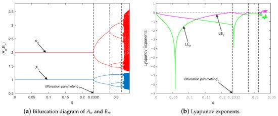
Figure 2 displays the bifurcation structure and corresponding Lyapunov exponent of System (7) as functions of the bifurcation parameter q. In Figure 2a, the fixed point remains stable within the interval (See Figure 3a,b), but becomes unstable at due to a period-doubling bifurcation. Additionally, Figure 2b shows the variation in the Lyapunov exponent, which takes on both positive () and negative values (), reflecting the system’s transition between chaotic and regular behaviors.
Figure 2.
(a) Period-doubling bifurcation diagram of System (7). (b) Corresponding Lyapunov exponents for the parameter values , , , and with initial conditions .
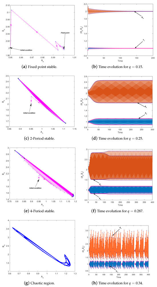
Figure 3.
Phase portraits and time evolutions of System (7) for different values of q: (a,b) , (c,d) , (e,f) , and (g,h) . The parameters are fixed as , , and .
Figure 3 illustrates the phase portraits corresponding to this case and the time evolutions, revealing a sequence of period-doubling bifurcations. The system exhibits periodic behavior with periods 2, 4, and 8, as shown in Figure 3c–f, respectively. This progression eventually leads to chaotic motion, which is evident in Figure 3g,h.
Example 2.
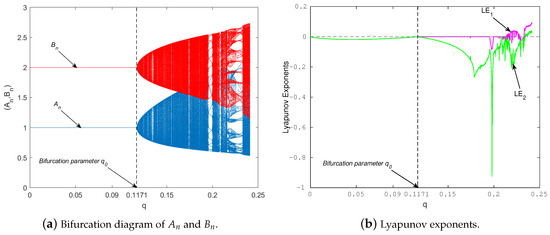
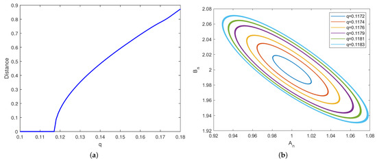
In this example, we examine System (7) with parameters , , , and , using the initial conditions . At the critical value , the system undergoes a Neimark–Sacker bifurcation at the positive fixed point . The corresponding Neimark–Sacker bifurcation diagrams for and are illustrated in Figure 4a. Furthermore, the Lyapunov exponents are plotted in Figure 4b. It is observed that the fixed point is locally asymptotically stable for , which is supported by the negative Lyapunov exponents (). At , the fixed point loses its stability. Consequently, a closed invariant curve emerges around the fixed point due to the Neimark–Sacker bifurcation (see Figure 4), and the diameter of this closed invariant curve increases as the value of q increases, accompanied by positive Lyapunov exponents () (see Figure 5).
Figure 4.
(a) The Neimark–Sacker bifurcation diagram of System (7). (b) Corresponding Lyapunov exponents for the parameter values , , , and with initial conditions .
Figure 5.
(a) Variation of the distance between the equilibrium point and the invariant closed curve as the parameter q changes. (b) Invariant closed curves corresponding to different values of q.
For further confirmation, we observe that with the parameter values , the Jacobian matrix of System (7) at the fixed point is given by
and its eigenvalues are and , satisfying . In this case, the discriminatory quantity is , which confirms the validity of Theorem 3.
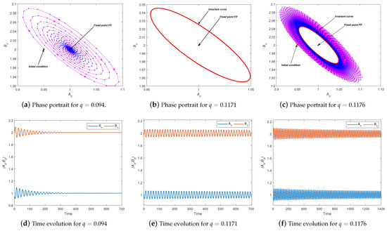
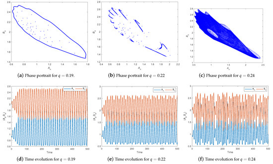
Figure 6 and Figure 7 present the phase portraits and time series of System (7) for different values of the bifurcation parameter q. At , the system settles into a stable equilibrium, as shown in Figure 6a,d. When , a closed invariant curve forms around the fixed point (see Figure 6b,e), signaling the onset of a Neimark–Sacker bifurcation. This curve remains and continues to attract nearby trajectories at (Figure 6c,f). As q increases, periodic behavior arises, particularly at and , as shown in Figure 7a,b,d,e. For higher values such as , the system transitions to chaotic dynamics, as evidenced by the complex attractors illustrated in Figure 7c,f.
Figure 6.
Phase portraits and time evolutions for different values of q are shown: (a,d) , (b,e) , (c,f) , using the parameter values , , and the initial conditions .
Figure 7.
Phase portraits and time evolutions for different values of q are shown: (a,d) , (b,e) , (c,f) , using the parameter values , , and the initial conditions .
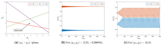
We now assess the performance of the state feedback control strategy in stabilizing System (7). To achieve this, we select the parameter values , , , and . Under these conditions, the marginal stability boundaries for the controlled System (23) are characterized by the following set of equations:
The lines , and enclose a triangular region in the -plane, defining the domain of stability for the controlled system. This stability zone is illustrated in Figure 8a. Selecting feedback gains and ensures that the fixed point P attains local asymptotic stability, as shown in Figure 8b. On the other hand, choosing and positions the point outside the stable region, resulting in instability (see Figure 8c). From an ecological perspective, implementing such feedback mechanisms can represent practical measures, such as controlled harvesting or habitat enhancement, to regulate species dynamics and mitigate chaotic or undesired oscillatory behavior.
Figure 8.
(a) Triangular stability region of the controlled System (23), bounded by , , and . (b,c) Time evolutions of and for and , respectively. The parameter values are , , , and .
9. 0-1 Test Algorithm
The 0-1 test, proposed by Gottwald and Melbourne [39], offers a simple and reliable approach for identifying chaotic dynamics. This method has been effectively applied to both continuous and discrete systems, as reported in [40,41,42]. The test analyzes a given time series and outputs a value in the range , where a value near 0 suggests regular (non-chaotic) behavior, and a value near 1 implies the presence of chaos.
Consider a time series consisting of M data points. The transformation of this series into the -plane is constructed as follows:
Let denote the j-th entry in the time series y, where , and let be a constant parameter. To quantify the growth behavior on the -plane, Gottwald and Melbourne [39] introduced the mean square displacement (MSD), which serves as an effective tool for detecting chaotic dynamics. The MSD is defined by the following expression:
To further evaluate the dynamical behavior, we calculate the asymptotic growth rate, denoted by , as follows:
where each is determined using the correlation coefficient formula:
with and . Here, represents a truncation threshold. The variance and covariance of the vectors x and y, each of length , calculated as
An increasing trend in indicates a shift toward chaotic dynamics, where the value of tends to 1. Conversely, in non-chaotic regimes (periodic or quasi-periodic), remains close to 0, assuming the boundedness of . In the -plane, bounded motion implies regular behavior, while a diffusion-like trajectory, akin to Brownian motion, signals chaos.
Example 3.

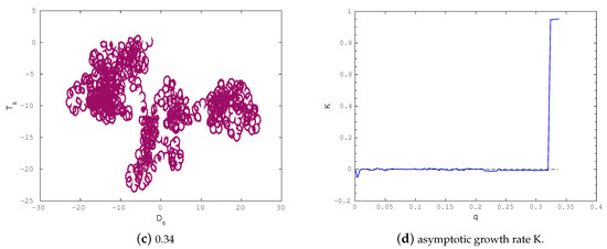
To further confirm the emergence of chaotic behavior in System (7), we utilize the 0-1 test for chaos under the parameter settings from Example 1: , , , and . The phase diagrams of the translation components and , together with the corresponding asymptotic growth rate , are presented in Figure 9 for several values of the bifurcation parameter q. For and , the trajectories remain confined in the -plane, indicating regular dynamics. In contrast, when , the system exhibits unbounded Brownian-like trajectories characteristic of chaotic motion. These outcomes are consistent with the bifurcation diagrams and the trends of the Lyapunov exponent shown in Figure 2b, offering additional evidence for the onset of chaos in the system.
Figure 9.
The phase plots of System (7) for various values of the parameter q: (a) , (b) , (c) . Panel (d) shows the corresponding asymptotic growth rate as a function of q.
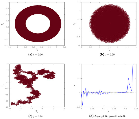
For the parameter set used in Example 2 (, , , and ), the phase plots of the translation components and , along with the associated asymptotic growth rate for different values of q, are shown in Figure 10. When and , the phase portraits in the -plane reveal confined trajectories, suggesting that the system exhibits periodic or quasi-periodic motion. However, for , the behavior becomes diffusive and unbounded, resembling a Brownian motion, indicative of chaos. These results are consistent with the bifurcation structure and the trend in the Lyapunov exponent displayed in Figure 4b, reinforcing the conclusion that the system undergoes a transition to chaos as q increases.
Figure 10.
The phase plots of System (7) for various values of the parameter q: (a) , (b) , (c) . Panel (d) shows the corresponding asymptotic growth rate as a function of q.
10. Results and Discussion
This section provides an exhaustive investigation of the Caputo fractional discrete-time modified Brusselator model. The outcomes have been organized around the most important phenomena investigated, which include fixed point stability, bifurcation structures, chaotic indicators, and numerical simulation validation.
The fractional-time Model (5) has initially been discretized using the piecewise-constant argument technique. We then calculated the system’s fixed point as . We employed linear stability analysis based on the Jacobian matrix evaluated at this equilibrium, as well as the Jury criterion adapted for fractional discrete-time systems, to establish precise constraints under which the fixed point remains locally asymptotically stable. According to Theorem 2, System (7) encounters a period-doubling bifurcation at the unique positive equilibrium point , if Conditions (16) hold. In particular, Figure 2 illustrates the bifurcation pattern and related Lyapunov exponent of System (7) as a function of the bifurcation parameter q. In Figure 2a, the fixed point appears stable inside the interval (as shown in Figure 3a), but turns unstable at due to a period-doubling bifurcation. Moreover, Figure 2b demonstrates the fluctuation in the Lyapunov exponent, which depends on a positive value ( and negative values (), exhibiting the system’s change from chaotic to regular manners. The phase portraits in Figure 3 exhibit a series of period-doubling bifurcations. The system has periodic behavior with periods 2, 4, and 8, as demonstrated in Figure 3c,e, correspondingly. The process of evolution ultimately generates chaotic motion, as depicted in Figure 3g.
According to Theorem 3, System (7) undergoes a Neimark–Sacker bifurcation at the fixed point as the bifurcation parameter varies in the neighborhood of , where the quantity is nonzero. Figure 6 and Figure 7 exhibit phase photographs and time series of System (7) for multiple values of the bifurcation parameter q. Figure 6a,d indicates that the system reaches a stable equilibrium at . A closed invariant curve develops around the equilibrium point at , indicating the beginning of a Neimark–Sacker bifurcation (see Figure 6b,e).
11. Conclusions
In this article, we investigated the Caputo fractional discrete-time modified Brusselator model in a comprehensive manner, emphasizing on its complicated dynamical features. The discretization of the fractional-time system utilizing the piecewise-constant argument enables us to thoroughly explore its dynamics. We determined highly accurate conditions for the fixed point’s local asymptotic stability using the Jury criterion and linear stability analysis. We discovered that, when the bifurcation parameter passes a critical threshold, the system encounters a period-doubling bifurcation, which ends up in several types of periodic behaviors that ultimately lead to chaotic dynamics. This shift was demonstrated utilizing numerical simulations, Lyapunov exponent analysis, and phase pictures, which straightforwardly demonstrated the origins of complex dynamics. Furthermore, the existence of a Neimark–Sacker bifurcation was theoretically verified and supported by numerical findings. The presence of complete invariant curves and quasi-periodic trajectories around the fixed point illustrates the model’s rich dynamical landscape, which is shaped by the interaction of fractional order and bifurcation parameter.
Author Contributions
Conceptualization, M.B.; Methodology, M.B. and M.B.A.; Software, M.B.; Formal analysis, M.B.; Validation, M.B.; Investigation, M.B.A.; Resources, M.B.A.; Writing—original draft, M.B. and M.B.A.; Writing—review and editing, M.B. and M.B.A.; Visualization, M.B.; Supervision, M.B. and M.B.A.; Funding acquisition, M.B.A. All authors have read and agreed to the published version of the manuscript.
Funding
This research received no external funding.
Data Availability Statement
The original contributions presented in this study are included in the article. Further inquiries can be directed to the corresponding author.
Conflicts of Interest
The authors declare no conflicts of interest.
References
- Asheghi, R. Stability and Hopf bifurcation analysis of a reduced Gierer-Meinhardt model. Int. J. Bifurc. Chaos 2021, 31, 2150149. [Google Scholar] [CrossRef]
- Chen, M.X.; Wang, T. Qualitative analysis and Hopf bifurcation of a generalized Lengyel-Epstein model. J. Math. Chem. 2023, 61, 166–192. [Google Scholar] [CrossRef]
- Wong, T.; Ward, M.J. Spot patterns in the 2-D Schnakenberg model with localized heterogeneities. Stud. Appl. Math. 2021, 146, 779–833. [Google Scholar] [CrossRef]
- Xu, C.; Mu, D.; Liu, Z.; Pang, Y.; Aouiti, C.; Tunc, O.; Ahmad, S.; Zeb, A. Bifurcation dynamics and control mechanism of a fractional–order delayed Brusselator chemical reaction model. Match 2023, 89, 73–106. [Google Scholar] [CrossRef]
- Xu, C.; Zhang, W.; Aouiti, C.; Liu, Z.; Li, P.; Yao, L. Bifurcation dynamics in a fractional-order Oregonator model including time delay. MATCH Commun. Math. Comput. Chem 2022, 87, 397–414. [Google Scholar] [CrossRef]
- Din, Q. Dynamics and Hopf bifurcation of a chaotic chemical reaction model. MATCH Commun. Math. Comput. Chem 2022, 88, 351–369. [Google Scholar] [CrossRef]
- Din, Q.; Haider, K. Discretization, bifurcation analysis and chaos control for Schnakenberg model. J. Math. Chem. 2020, 58, 1615–1649. [Google Scholar] [CrossRef]
- Kol’tsov, N. Chaotic oscillations in four-step chemical reaction. Russ. J. Phys. Chem. B 2017, 11, 1047–1048. [Google Scholar] [CrossRef]
- Monwanou, A.V.; Koukpémèdji, A.; Ainamon, C.; Nwagoum Tuwa, P.; Miwadinou, C.; Chabi Orou, J. Nonlinear Dynamics in a Chemical Reaction under an Amplitude-Modulated Excitation: Hysteresis, Vibrational Resonance, Multistability, and Chaos. Complexity 2020, 2020, 8823458. [Google Scholar] [CrossRef]
- Bodale, I.; Oancea, V.A. Chaos control for Willamowski–Rössler model of chemical reactions. Chaos Solitons Fractals 2015, 78, 1–9. [Google Scholar] [CrossRef]
- Binous, H.; Bellagi, A. Introducing nonlinear dynamics to chemical and biochemical engineering graduate students using MATHEMATICA©. Comput. Appl. Eng. Educ. 2019, 27, 217–235. [Google Scholar] [CrossRef]
- Aruna, K.; Okposo, N.I.; Raghavendar, K.; Inc, M. Analytical solutions for the Noyes Field model of the time fractional Belousov Zhabotinsky reaction using a hybrid integral transform technique. Sci. Rep. 2024, 14, 25015. [Google Scholar] [CrossRef]
- Chi, Z. Analytical and numerical computation of self-oscillating gels driven by the Belousov-Zhabotinsky reaction. Phys. Scr. 2024, 99, 025229. [Google Scholar] [CrossRef]
- Karimov, A.; Kopets, E.; Karimov, T.; Almjasheva, O.; Arlyapov, V.; Butusov, D. Empirically developed model of the stirring-controlled Belousov–Zhabotinsky reaction. Chaos Solitons Fractals 2023, 176, 114149. [Google Scholar] [CrossRef]
- Prigogine, I.; Lefever, R. Symmetry breaking instabilities in dissipative systems. II. J. Chem. Phys. 1968, 48, 1695–1700. [Google Scholar] [CrossRef]
- Chen, M. Hopf Bifurcation and Self–Organization Pattern of a Modified Brusselator Model. MATCH Commun. Math. Comput. Chem. 2023, 90, 581–607. [Google Scholar] [CrossRef]
- Khan, M.A.; Khan, M.S.; Din, Q.; Abdelfattah, W. Codimension-one and codimension-two bifurcations of a modified Brusselator model. Int. J. Dyn. Control 2025, 13, 1–20. [Google Scholar] [CrossRef]
- Strogatz, S.H. Nonlinear Dynamics and Chaos: With Applications to Physics, Biology, Chemistry, and Engineering; Chapman and Hall/CRC: Boca Raton, FL, USA, 2024. [Google Scholar]
- Berkal, M.; Almatrafi, M.B. Bifurcation and Stability of Two-Dimensional Activator–Inhibitor Model with Fractional-Order Derivative. Fractal Fract. 2023, 7, 344. [Google Scholar] [CrossRef]
- Liu, Y.; Li, X. Dynamics of a discrete predator-prey model with Holling-II functional response. Int. J. Biomath. 2021, 14, 2150068. [Google Scholar] [CrossRef]
- Yousef, A.; Rida, S.; Gouda, Y.G.; Zaki, A. Dynamical behaviors of a fractional-order predator–prey model with Holling type iv functional response and its discretization. Int. J. Nonlinear Sci. Numer. Simul. 2019, 20, 125–136. [Google Scholar] [CrossRef]
- Almatrafi, M.B.; Berkal, M. Bifurcation analysis and chaos control for fractional predator-prey model with Gompertz growth of prey population. Mod. Phys. Lett. B 2024, 39, 2550103. [Google Scholar] [CrossRef]
- Berkal, M.; Navarro, J.F.; Hamada, M.; Semmar, B. Qualitative behavior for a discretized conformable fractional-order predator–prey model. J. Appl. Math. Comput. 2025, 71, 4815–4837. [Google Scholar] [CrossRef]
- Almatrafi, M.B.; Berkal, M.; Hamada, M.Y. Qualitative Behavior of a Discrete-Time Predator–Prey Model With Holling-Type III Functional Response and Gompertz Growth of Prey. Math. Meth. Appl. Sci. 2025, 2013, 13100–13112. [Google Scholar] [CrossRef]
- Berkal, M.; Navarro, J.F. Qualitative behavior of a two-dimensional discrete-time prey–predator model. Comput. Math. Methods 2021, 3, e1193. [Google Scholar] [CrossRef]
- Liu, X.; Xiao, D. Complex dynamic behaviors of a discrete-time predator–prey system. Chaos Solitons Fractals 2007, 32, 80–94. [Google Scholar] [CrossRef]
- Din, Q. Bifurcation analysis and chaos control in discrete-time glycolysis models. J. Math. Chem. 2018, 56, 904–931. [Google Scholar] [CrossRef]
- Din, Q.; Elsadany, A.; Ibrahim, S. Bifurcation analysis and chaos control in a second-order rational difference equation. Int. J. Nonlinear Sci. Numer. Simul. 2018, 19, 53–68. [Google Scholar] [CrossRef]
- Almatrafi, M.; Berkal, M. Bifurcation analysis and chaos control for prey-predator model with Allee effect. Int. J. Anal. Appl. 2023, 21, 131. [Google Scholar] [CrossRef]
- Ma, R.; Bai, Y.; Wang, F. Dynamical behavior analysis of a two-dimensional discrete predator-prey model with prey refuge and fear factor. J. Appl. Anal. Comput. 2020, 10, 1683–1697. [Google Scholar] [CrossRef]
- Mukherjee, D. Dynamics of a discrete-time ecogenetic predator-prey model. Commun. Biomath. Sci. 2022, 5, 161–169. [Google Scholar] [CrossRef]
- Berkal, M.; Navarro, J.F. Qualitative behavior of a chemical reaction system with fractional derivatives. Rocky Mt. J. Math. 2025, 55, 11–24. [Google Scholar] [CrossRef]
- Berkal, M.; Navarro, J.F. Dynamics of a discrete-time predator-prey system with ratio-dependent functional response. Miskolc Math. Notes 2025, 26, 81–99. [Google Scholar] [CrossRef]
- Kartal, S.; Gurcan, F. Discretization of conformable fractional differential equations by a piecewise constant approximation. Int. J. Comput. Math. 2019, 96, 1849–1860. [Google Scholar] [CrossRef]
- Din, Q.; Zulfiqar, M.A. Qualitative behavior of a discrete predator–prey system under fear effects. Z. Naturforschung A 2022, 77, 1023–1043. [Google Scholar] [CrossRef]
- Elaydi, S.N.; Elaydi, S.N. Systems of Difference Equations. In An Introduction to Difference Equations; Springer: New York, NY, USA, 1996; pp. 113–162. [Google Scholar]
- Gümüş, O.A.; Selvam, A.G.M.; Janagaraj, R. Neimark–Sacker bifurcation and control of chaotic behavior in a discrete-time plant-herbivore system. J. Sci. Arts 2022, 22, 549–562. [Google Scholar] [CrossRef]
- Chen, G.; Dong, X. From Chaos to Order: Methodologies, Perspectives and Applications; World Scientific: Singapore, 1998; Volume 24. [Google Scholar]
- Gottwald, G.A.; Melbourne, I. A new test for chaos in deterministic systems. Proc. R. Soc. London. Ser. A Math. Phys. Eng. Sci. 2004, 460, 603–611. [Google Scholar] [CrossRef]
- Martinovič, T. Alternative approaches of evaluating the 0-1 test for chaos. Int. J. Comput. Math. 2020, 97, 508–521. [Google Scholar] [CrossRef]
- Terry-Jack, M.; O’Keefe, S. Classifying 1D elementary cellular automata with the 0-1 test for chaos. Phys. D Nonlinear Phenom. 2023, 453, 133786. [Google Scholar] [CrossRef]
- Xin, B.; Li, Y. 0-1 Test for Chaos in a Fractional Order Financial System with Investment Incentive. Abstr. Appl. Anal. 2013, 2013, 876298. [Google Scholar] [CrossRef]
Disclaimer/Publisher’s Note: The statements, opinions and data contained in all publications are solely those of the individual author(s) and contributor(s) and not of MDPI and/or the editor(s). MDPI and/or the editor(s) disclaim responsibility for any injury to people or property resulting from any ideas, methods, instructions or products referred to in the content. |
© 2025 by the authors. Licensee MDPI, Basel, Switzerland. This article is an open access article distributed under the terms and conditions of the Creative Commons Attribution (CC BY) license (https://creativecommons.org/licenses/by/4.0/).