Article

A New Weibull–Rayleigh Distribution: Characterization, Estimation Methods, and Applications with Change Point Analysis

1
Department of Statistics, Faculty of Science, King Abdulaziz University, Jeddah 21589, Saudi Arabia
2
Department of Mathematics, King Khalid University, Abha 61421, Saudi Arabia
*
Author to whom correspondence should be addressed.
Axioms 2025, 14(9), 649; https://doi.org/10.3390/axioms14090649
Submission received: 29 June 2025 / Revised: 2 August 2025 / Accepted: 20 August 2025 / Published: 22 August 2025
(This article belongs to the Special Issue Probability, Statistics and Estimations, 2nd Edition)

Abstract

Many scholars are interested in modeling complex data in an effort to create novel probability distributions. This article proposes a novel class of distributions based on the inverse of the exponentiated Weibull hazard rate function. A particular member of this class, the Weibull–Rayleigh distribution (WR), is presented with focus. The WR features diverse probability density functions, including symmetric, right-skewed, left-skewed, and the inverse J-shaped distribution which is flexible in modeling lifetime and systems data. Several significant statistical features of the suggested WR are examined, covering the quantile, moments, characteristic function, probability weighted moment, order statistics, and entropy measures. The model accuracy was verified through Monte Carlo simulations of five different statistical estimation methods. The significance of WR is demonstrated with three real-world data sets, revealing a higher goodness of fit compared to other competing models. Additionally, the change point for the WR model is illustrated using the modified information criterion (MIC) to identify changes in the structures of these data. The MIC and curve analysis captured a potential change point, supporting and proving the effectiveness of WR distribution in describing transitions.

1. Introduction

In many applied areas such as engineering, medicine, insurance, and economics, probability distributions are widely used to model, analyze, and predict data behavior. The accuracy with which we have performed statistical inference would depend, to a large extent, on the quality of fit of the selected probability distribution to the underlying data patterns. However, many traditional distributions are often not flexible and accurate enough to model complex datasets, which has led to the development of new distribution models that possess more flexibility.
The T-X method proposed by [1] is one of the popular approaches for creating classes of distributions. This technique consists in combining a base distribution F ( x ) with an upper bound function W ( F ( x ) ) to obtain different families of distributions. Based on this idea, some remarkable families and distributions have been constructed, such as the Gompertz–G family by [2], exponentiated T-X family by [3], the transmuted Topp–Leone–G family by [4], and the odd Nadarajah–Haghighi family by [5].
In a very recent research article [6], a new family based on the T-X approach was proposed by introducing m c ( x ) as an upper bound of the integral, where m c ( x ) is the exponentiated inverse of the hazard function (HF), and c > 0 is a shape parameter that affects the weight of the distribution. The cumulative distribution function (CDF), and the probability density function (PDF) of the family can be obtained as follows:
F ( x ) = m c x g ( t ) d t = G m c x , x R , c > 0 ,
f ( x ) = d d x m c x g m c x .
This approach has been designed to successfully achieve more flexible distributions that can accurately fit real data.
Therefore, this article will introduce a new class of distributions based on the HF of the Weibull distribution. The CDF and PDF for this new class are defined as follows.
F ( x ) = 0 x 1 λ θ λ α g ( t ) d t = G x 1 λ θ λ α ,
f ( x ) = x x 1 λ θ λ α g x 1 λ θ λ α .
The Weibull distribution is one of the most popular life and reliability data distributions, because of its flexibility to model increasing and decreasing failure rates. As a versatile tool in temporal data analysis, it has been shown to be effective in capturing time-related failure behaviors, especially in the analysis of temporal failure behaviors related to reliability and survivability and the response of physical or biological systems under various changing conditions.
The Weibull distribution, while versatile, is insufficient for modeling data that exhibit non-monotonic failure behavior. In order to address these limitations, various extended families have been introduced, with the Weibull-G proposed by [7] being the most notable. This involves inserting a baseline distribution function into the Weibull structure to increase the flexibility of the model. In addition, several families were established such as the generalized Weibull family introduced by [8], the truncated Weibull-G family, introduced by [9], as well as the extended odd Weibull-G given in [10], and a new power generalized Weibull-G from [11]. These families can be used to improve modeling for real-world data that have complex tail behavior or varying hazard rate shapes by incorporating additional shape parameters to improve flexibility.
The Rayleigh distribution, which is a special case of the Weibull distribution, is one of the oldest and most recognized distributions in fields such as signal analysis, radar systems, and reliability. The significance of this distribution is that it has a straightforward and interpretable design. It has frequently been used to describe multipath fading in wireless communication systems by [12]. Within fading-shadowing channels [13] showed that it is also the basic reference structure for models with more involved anatomy. Furthermore, the extended form of the Rayleigh distribution has been widely investigated in reliability analysis and parameter estimation, as presented by [14].
In such contexts, change-point (CP) analysis has become a useful statistical tool to detect discontinuities and turning points in real-world data. This approach is used to identify the points in time at which a distribution changes significantly either in mean, variance, or overall distributional shape. It has found its extensive application from quality control, medical diagnosis and performance monitoring to time-series analysis in dynamical or industrial environments. The techniques used are based on classical tests, information criteria, and data-driven algorithms, making it an advanced technique to identify unobserved changing signals in data. In addition to its numerous applications in applied sciences, CP analysis is also effective in analyzing probability distributions, particularly in detecting structural changes in distributional characteristics, such as changes in parameters or changes in shape [15,16,17,18,19].
Inspired by the efficacy of the novel methodology in [6] to generate more flexible distributions that accurately correspond to empirical data, this article aims to integrate the capabilities of the Weibull distribution with the features of the Rayleigh distribution. This will yield a distribution capable of modeling complex data with non-monotonic failure rates, reflecting real-world scenarios where system or component failure rates vary over time, a phenomenon prevalent in engineering, finance, healthcare, and other sectors. The newly developed flexible form of the Weibull–Rayleigh distribution (WR) will effectively capture structural changes in the data. This is especially advantageous in contexts where distributional characteristics undergo sudden changes, such as alterations in operational conditions or treatment effects. The WR distribution integrates the CP analysis using MIC to determine the location of structural changes.
The structure of the paper is outlined as follows: Section 2 introduces the new Weibull–Rayleigh distribution. Some statistical properties of WR are investigated in Section 3. Five methods of estimation are used to estimate the WR parameters in Section 4. Section 5 presents a simulation study to evaluate the performance of the estimators. In Section 6, three real-world data sets are analyzed to emphasize the importance of the WR distribution and demonstrate CP detection. Finally, Section 7 reports the findings and concludes the article.

2. The Weibull–Rayleigh Distribution

Consider replacing the g and G in Equations (3) and (4) by the PDF and CDF of the Rayleigh distribution, then the CDF of the proposed WR distribution is given by
F ( x ) = 1 e 1 2 β 2 x 1 λ θ λ 2 α , x > 0 ,
and the corresponding PDF of the WR distribution is obtained as follows:
f ( x ) = α 1 λ x 2 α ( 1 λ ) 1 β 2 ( θ λ ) 2 α e 1 2 β 2 x 1 λ θ λ 2 α .
where α is a shape parameter, β and θ > 0 are scale parameters, and 0 < λ < 1 is the major lever for skew and behavior around 0.
The survival function S ( x ) and the HF, denoted by H ( x ) for the WR distribution, are given by the following expressions:
S ( x ) = e 1 2 β 2 x 1 λ θ λ 2 α ,
H ( x ) = α 1 λ x 2 α ( 1 λ ) 1 β 2 ( θ λ ) 2 α .

2.1. Graphical Representations of the WR Distribution

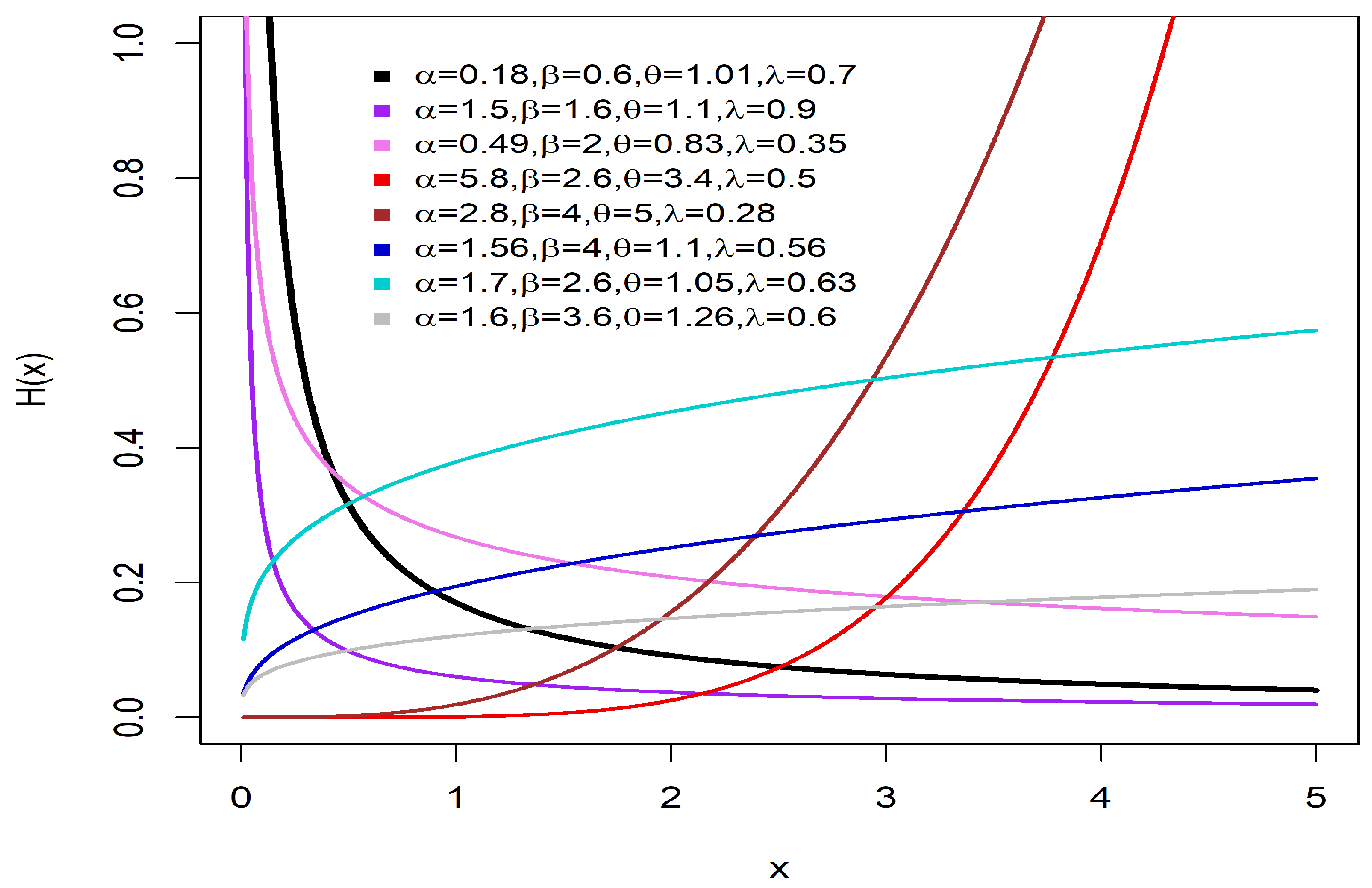
The PDF and HF of WR distribution for some parameter values are illustrated in Figure 1 and Figure 2, respectively.
As can be observed from Figure 1, The WR pdf plots have different shapes that include symmetric, right-skewed, left-skewed and reverse J-shaped. The HF for the WR in Figure 2 takes symmetric, asymmetrical J-shaped, and inverted J-shaped forms. This provides strong evidence of the high flexibility of the WR distribution to fit real-world data.

2.2. Special Cases of the WR Distribution

  • The WR takes the form of the Rayleigh distribution when
    θ = λ = 1 , a n d α = 1 2 .
  • The WR distribution takes the form of the Weibull distribution when
    θ = 1 , α = 1 2 , β = 1 2 β , a n d x = λ y λ 1 1 λ .
  • The WR distribution takes the form of the Weibull exponential distribution when
    α = α 2 , β = 1 2 β α , a n d x = λ 2 y 1 1 λ .
  • The WR distribution takes the form of the Rayleigh Rayleigh distribution when
    α = β = 1 , θ = 2 θ 2 , a n d x = y 2 1 λ .
  • The WR distribution takes the form of the Gompertz distribution when
    α = 1 2 , β = 1 2 , θ = 1 θ , a n d x = e λ y 1 1 1 λ .
  • The WR distribution takes the form of the exponentiated exponential distribution when θ = 1 , β = 1 2 , a n d x = λ l n 1 1 e λ y α 1 2 α 1 1 λ .
  • The WR distribution takes the form of the Weibull–Lomax distribution when
    α = α 2 , β = 1 2 , a n d x = λ θ 2 log 1 + λ y 1 1 λ .

3. Statistical Properties of the WR Distribution

3.1. Quantile, Median, Skewness and Kurtosis

The quantile function, denoted by x p = Q ( p ) , of the WR distribution is expressed as:
x p = θ λ 2 β 2 l n ( 1 p ) 1 2 α 1 1 λ ,
then, the median can be calculated by setting p = 0.5 in Equation (9):
x 0.5 = θ λ 2 β 2 l n ( 0.5 ) 1 2 α 1 1 λ .
Skewness and kurtosis are obtained as follows:
S k = x 0.75 2 x 0.5 + x 0.25 x 0.75 x 0.5 ,
and
K u r = x 0.875 x 0.625 x 0.375 + x 0.125 x 0.75 x 0.5 ,
where x ( . ) denotes the quantile function of the WR.

3.2. Moments

If X W R ( α , β , θ , λ ) , then the rth moment of X can be expressed as
μ r = E ( X r ) = 0 x r f ( x ) d x , = 0 x r · α 1 λ x 2 α ( 1 λ ) 1 β 2 ( θ λ ) 2 α e 1 2 β 2 x 1 λ θ λ 2 α d x .
Setting w = 1 2 β 2 x 1 λ θ λ 2 α , we obtain
μ r = 0 α ( 1 λ ) β 2 ( θ λ ) 2 α 2 β 2 w ( θ λ ) 2 α 1 2 α ( 1 λ ) 2 α ( 1 λ ) + r 1 e w 2 β 2 ( θ λ ) 2 α 2 α ( 1 λ ) 2 β 2 w ( θ λ ) 2 α 1 2 α ( 1 λ ) 1 d w .
Hence, the rth moment of the WR distribution can be expressed as
μ r = 2 β 2 ( θ λ ) 2 α r 2 α ( 1 λ ) Γ r 2 α ( 1 λ ) + 1 .
The mean, the second moment and variance of WR are
μ 1 = E ( X ) = 2 β 2 ( θ λ ) 2 α 1 2 α ( 1 λ ) Γ 1 2 α ( 1 λ ) + 1 ,
μ 2 = E ( X 2 ) = 2 β 2 ( θ λ ) 2 α 1 α ( 1 λ ) Γ 1 α ( 1 λ ) + 1 ,
σ 2 = μ 2 μ 1 2 , = 2 β 2 ( θ λ ) 2 α 1 α ( 1 λ ) Γ 1 α ( 1 λ ) + 1 Γ 1 2 α ( 1 λ ) + 1 2 .

3.3. Moment Generating Function (MGF)

The MGF of WR distribution is given by
M X ( t ) = r = 0 t r r ! μ r = r = 0 t r r ! 2 β 2 ( θ λ ) 2 α r 2 α ( 1 λ ) Γ r 2 α ( 1 λ ) + 1 .

3.4. Characteristic Function

The characteristic function of WR distribution is given by
ϕ X t = E e i t x = r = 0 i t r r ! μ r = r = 0 i t r r ! 2 β 2 ( θ λ ) 2 α r 2 α ( 1 λ ) Γ r 2 α ( 1 λ ) + 1 .

3.5. Probability Weighted Moment (PWM)

The PWM of the random variable (RV) X, which follows the WR distribution, can be represented as follows:
E X r F ( X ) s = x r f ( x ) F ( x ) s d x , r , s 0 .
Substituting Equations (5) and (6) in (21), we get
E X r F ( X ) s = 0 x r α 1 λ x 2 α ( 1 λ ) 1 β 2 ( θ λ ) 2 α e 1 2 β 2 x 1 λ θ λ 2 α 1 e 1 2 β 2 x 1 λ θ λ 2 α s d x .
Then, by applying the generalized series expansion:
( 1 z ) n = i = 0 ( 1 ) i n i z i , | Z | < 1 ,
we obtain
E X r F ( X ) s = α ( 1 λ ) β 2 θ λ 2 α i = 0 ( 1 ) i s i 0 x 2 α ( 1 λ ) + r 1 e ( i + 1 ) 2 β 2 x 1 λ θ λ 2 α d x .
Substituting w = ( i + 1 ) 2 β 2 x 1 λ θ λ 2 α , we have
E X r F ( X ) s = α ( 1 λ ) β 2 ( θ λ ) 2 α i = 0 ( 1 ) i s i 0 2 β 2 θ λ 2 α i + 1 w 1 2 α ( 1 λ ) 2 α ( 1 λ ) + r 1 β 2 ( θ λ ) 2 α α ( 1 λ ) ( i + 1 ) 2 β 2 θ λ 2 α i + 1 w 1 2 α ( 1 λ ) 1 e w d w .
Therefore, the PWM for the WR distribution is given by:
E X r F ( X ) s = i = 0 ( 1 ) i i + 1 s i 2 β 2 θ λ 2 α i + 1 r 2 α ( 1 λ ) Γ r 2 α ( 1 λ ) + 1 .

3.6. Order Statistics

Order statistics describe the distribution of ordered values in a random sample (RS). Given independent and identically distributed variables X 1 : n < X 2 : n < X 3 : n < < X n : n , the rth order statistic x r : n is:
f r : n ( x ) = f ( x ) β ( r , n r + 1 ) v = 0 n r ( 1 ) v n r v F v + r 1 ( x ) ,
where β ( r , n r + 1 ) = Γ ( r ) Γ ( n r + 1 ) Γ ( n + 1 ) .
By substituting the CDF and PDF of the WR distribution in Equations (5) and (6) we get
f r : n ( x ) = α 1 λ x 2 α ( 1 λ ) 1 β 2 ( θ λ ) 2 α β ( r , n r + 1 ) e 1 2 β 2 x 1 λ θ λ 2 α v = 0 n r ( 1 ) v n r v 1 e 1 2 β 2 x 1 λ θ λ 2 α v + r 1 ,
and then applying the series expansion
( 1 z ) n = i = 0 n ( 1 ) i n i z i .
Then, the order statistics of the WR distribution is obtained as
f r : n ( x ) = α ( 1 λ ) β 2 ( θ λ ) 2 α v = 0 n r i = 0 v + r 1 ( 1 ) i + v β ( r , n r + 1 ) n r v v + r 1 i x 2 α ( 1 λ ) 1 e i + 1 2 β 2 x 1 λ θ λ 2 α .

3.7. Shannon Entropy

The Shannon entropy is a measure of the uncertainty of a probability distribution and it is the average information generated by a RV X. It is defined as:
S E x = E l o g f ( x ) .
Inserting the PDF in Equation (6) into Equation (31), then
S E x = 0 α 1 λ x 2 α ( 1 λ ) 1 β 2 ( θ λ ) 2 α e 1 2 β 2 x 1 λ θ λ 2 α l o g α ( 1 λ ) β 2 ( θ λ ) 2 α + 2 α ( 1 λ ) 1 l o g ( x ) 1 2 β 2 x 1 λ θ λ 2 α d x .
Consider the following series expansion.
l o g ( x ) = k = 1 ( 1 ) k + 1 k ( x 1 ) k ,
and subsequently using the generalized series expansion in Equation (23), we have
S E x = α ( 1 λ ) β 2 ( θ λ ) 2 α l o g α ( 1 λ ) β 2 ( θ λ ) 2 α 0 x 2 α ( 1 λ ) 1 e 1 2 β 2 x 1 λ θ λ 2 α d x + α ( 1 λ ) 2 β 4 ( θ λ ) 4 α 0 x 4 α ( 1 λ ) 1 e 1 2 β 2 x 1 λ θ λ 2 α d x α ( 1 λ ) β 2 ( θ λ ) 2 α 2 α ( 1 λ ) 1 k = 1 i = 0 ( 1 ) i + 1 k k i 0 x 2 α ( 1 λ ) + i 1 e 1 2 β 2 x 1 λ θ λ 2 α d x ,
Setting w = 1 2 β 2 x 1 λ θ λ 2 α , then
S E x = l o g α ( 1 λ ) β 2 ( θ λ ) 2 α + 0 w e w d w ( 2 α ( 1 λ ) 1 ) k = 1 i = 0 ( 1 ) i + 1 k k j 0 2 β 2 ( θ λ ) 2 α w i 2 α ( 1 λ ) e w d w .
Therefore, the Shannon entropy of the WR distribution is
S E x = l o g α ( 1 λ ) β 2 ( θ λ ) 2 α ( 2 α ( 1 λ ) 1 ) k = 1 i = 0 ( 1 ) i + 1 k k j 2 β 2 ( θ λ ) 2 α i 2 α ( 1 λ ) Γ i 2 α ( 1 λ ) + 1 + 1 .

3.8. Rényi Entropy

The Rényi entropy generalizes the Shannon entropy by quantifying the uncertainty of a probability distribution, with the sensitivity defined by the order parameter u. It is defined as
R E X ( u ) = 1 1 u l o g f u ( x ) d x , u > 0 , u 1 .
By substituting the PDF given in Equation (6), we obtain the following expression for the Rényi entropy.
R E X ( u ) = 1 1 u l o g 0 α 1 λ x 2 α ( 1 λ ) 1 β 2 ( θ λ ) 2 α e 1 2 β 2 x 1 λ θ λ 2 α u d x ,
To evaluate the integral part, we substitute w = u 2 β 2 x 1 λ θ λ 2 α , then
0 α 1 λ x 2 α ( 1 λ ) 1 β 2 ( θ λ ) 2 α e 1 2 β 2 x 1 λ θ λ 2 α u d x = 1 u α ( 1 λ ) β 2 ( θ λ ) 2 α u 1 2 β 2 ( θ λ ) 2 α u 1 u 2 α ( 1 λ ) + u 1 Γ 1 u 2 α ( 1 λ ) + u ,
Therefore, the Rényi entropy of the WR distribution is
R E X ( u ) = l o g 2 α ( 1 λ ) 1 2 α ( 1 λ ) + u 1 u l o g ( u ) + 1 2 α ( 1 λ ) l o g 2 β 2 ( θ λ ) 2 α + 1 1 u l o g Γ 1 u 2 α ( 1 λ ) + u .

4. Estimation Methods

In this work, five methods of estimation will be used to estimate the parameters of the WR distribution: Maximum Likelihood (ML), Percentile Estimation (PE), Least Squares Estimation (LSE), Weighted Least Squares (WLS), and Cramér–von Mises Minimum Distance Estimation (CVM). These methods differ in their estimation approach and the efficiency they offer.

4.1. Maximum Likelihood

Consider a RS x 1 , x 2 , x 3 , , x n drawn from WR distribution, then the log-likelihood function is:
l = n l o g ( α ) + n l o g ( 1 λ ) 2 n l o g ( β ) 2 α n l o g ( θ λ ) + i = 1 n 2 α ( 1 λ ) 1 l o g ( x i ) 1 2 β 2 i = 1 n x i 1 λ θ λ 2 α ,
To obtain the ML estimates of the parameters, we take the partial derivatives of Equation (41) concerning each parameter, set the resulting expressions equal to zero, and solve the resulting system of equations as follows:
l α = n α 2 n l o g ( θ λ ) + i = 1 n 2 ( 1 λ ) l o g ( x i ) 1 β 2 i = 1 n x i 1 λ θ λ 2 α l o g x i 1 λ θ λ ,
l β = 2 n β + 1 β 3 i = 1 n x i 1 λ θ λ 2 α ,
l θ = 2 α n θ + α θ β 2 i = 1 n x i 1 λ θ λ 2 α ,
l λ = n 1 λ + 2 α n λ + i = 1 n log ( x i ) + α β 2 i = 1 n λ log ( x i ) + 1 λ x i 1 λ θ λ 2 α .
The estimates of the parameters are derived by solving the system of nonlinear Equations (42)–(45) through iterative optimization methods. Such methods can be easily applied using statistical software tools, including packages available in R [20].

4.2. Percentile Estimation

Let x 1 , x 2 , x 3 , , x n denote a RS of size n from a WR distribution. The PE method can be developed as:
P E α , β , θ , λ = i = 1 n x i θ λ 2 β 2 l n ( 1 p i ) 1 2 α 1 1 λ 2 ,
where p i = i n + 1 a n d i = 1 , 2 , 3 , , n .
To determine the parameters of WR distribution, the PE method minimizes the squared differences of the actual sample order statistics and the corresponding predicted values which are calculated from the given percentiles.

4.3. Ordinary Least Squares Estimators

Let x 1 , x 2 , x 3 , , x n be a RS of size n from WR distribution. The parameters are optimized by minimizing the sum of the squares of the differences. Consequently, the estimate of the parameters is obtained based on ordinary LSE by minimizing the following:
L S E = i = 1 n F W R x i i n + 1 2 = i = 1 n 1 e 1 2 β 2 x i 1 λ θ λ 2 α i n + 1 2 .

4.4. Weighted Least Squares Estimators

Let x 1 , x 2 , x 3 , , x n denote a RS of size n from the WR distribution. The estimate of the WR parameters based on WLS will be obtained by minimizing
W L S = i = 1 n n + 1 2 n + 2 i n i + 1 F W R x i i n + 1 2 = i = 1 n n + 1 2 n + 2 i n i + 1 1 e 1 2 β 2 x i 1 λ θ λ 2 α i n + 1 2 .

4.5. Cramér–von Mises Minimum Distance

The CVM is based on the assumption that the estimated CDF is held in some sense close to the empirical CDF. Therefore, the CVM estimates of the WR parameters can be found by minimizing the expression.
C V M = 1 12 n + i = 1 n F W R ( x i ) 2 i 1 2 n 2 = 1 12 n + i = 1 n 1 e 1 2 β 2 x i 1 λ θ λ 2 α 2 i 1 2 n 2 .

5. Simulation Study

A Monte Carlo simulation study is presented to compare the performance of the five estimation methods ML, PE, LSE, WLS and CVM to estimate the parameters of the WR distribution. We generate data from the WR distribution using Equation (9) with p u n i f o r m ( 0 , 1 ) . A wide range of sample sizes (n) are considered (n = 20, 50, 100, 200, 300, 500) and in each case, we perform 1000 independent repetitions. For the simulation, we consider the following five sets of parameter values.
  • Set I: ( α = 4.27 , β = 0.8 , θ = 3.9 , a n d λ = 0.52 ) .
  • Set II: ( α = 5.6 , β = 2.4 , θ = 2.8 , a n d λ = 0.4 ) .
  • Set III: ( α = 1.39 , β = 0.32 , θ = 0.8 , a n d λ = 0.6 ) .
  • Set IV: ( α = 2.5 , β = 1.8 , θ = 1.44 , a n d λ = 0.29 ) .
  • Set V: ( α = 3.5 , β = 0.38 , θ = 0.28 , a n d λ = 0.33 ) .
The parameters are estimated using the ‘optim’ function in R package [20]. In addition, we calculate the absolute values of mean bias (Bias) and mean squared error (MSE) for each of them are given by:
B i a s ( φ ^ ) = 1 n i = 1 n ( φ ^ i φ ) , M S E ( φ ^ ) = 1 n i = 1 n ( φ ^ i φ ) 2 ,
where ( φ ) is the true value of a parameter, ( φ ^ ) is its estimate and n is the sample size.
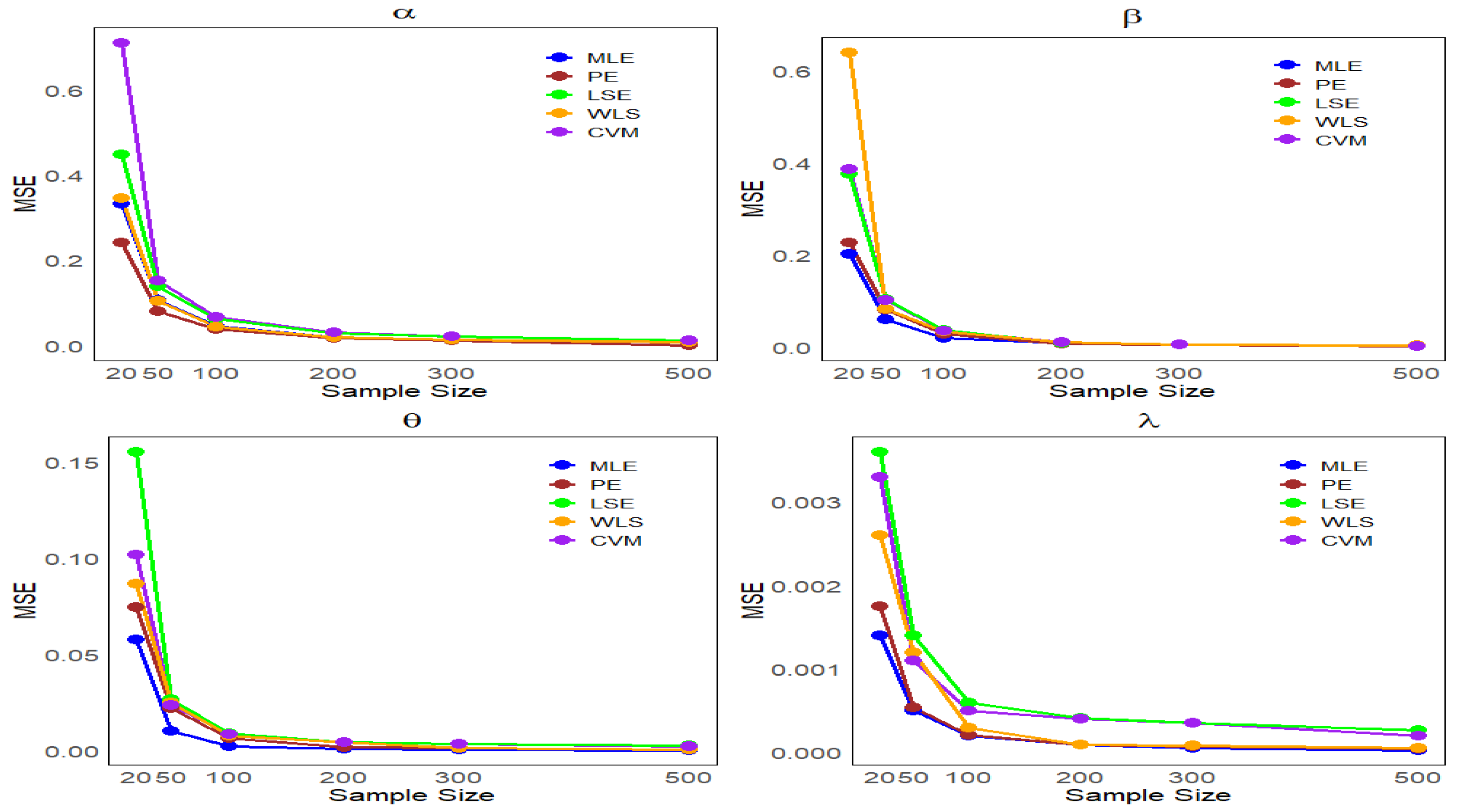
The results presented in Table 1, Table 2, Table 3, Table 4 and Table 5 show that the accuracy of the WR parameter estimates improves with increasing sample size, suggesting that the average φ ^ ’s converge to the actual parameter values ( φ ). Furthermore, Figure 3, Figure 4, Figure 5, Figure 6 and Figure 7 also illustrate the comparison among estimation methods in terms of MSE for various sample sizes. According to these comparisons, the ML and PE methods outperform other methods in terms of stability and accuracy. The calculations were performed with the software package R (v4.3.2; R Core Team 2023) [20].

6. Applications

This section demonstrates the applicability of the WR distribution to real-life data, indicating that WR provides a superior fit compared to several established distributions.
Failure times of 50 components (per 1000 h).
The following is the dataset, which is taken from [21] and represents the failure times of 50 components (in 1000 h). The observations are:
0.036, 0.058, 0.061, 0.074, 0.078, 0.086, 0.102, 0.103, 0.114, 0.116, 0.148, 0.183, 0.192, 0.254, 0.262, 0.379, 0.381, 0.538, 0.570, 0.574, 0.590, 0.618, 0.645, 0.961, 1.228, 1.600, 2.006, 2.054, 2.804, 3.058, 3.076, 3.147, 3.625, 3.704, 3.931, 4.073, 4.393, 4.534, 4.893, 6.274, 6.816, 7.896, 7.904, 8.022, 9.337, 10.940, 11.020, 13.880, 14.730, 15.080.
Carbon fiber breaking stress (GPa).
The second data set scoured from [22], comprises 100 observations on breaking stress of carbon fibers (in Gba):
0.39, 0.81, 0.85, 0.98, 1.08, 1.12, 1.17, 1.18, 1.22, 1.25, 1.36, 1.41, 1.47, 1.57, 1.57, 1.59, 1.59, 1.61, 1.61, 1.69, 1.69, 1.71, 1.73, 1.80, 1.84, 1.84, 1.87, 1.89, 1.92, 2, 2.03, 2.03, 2.05, 2.12, 2.17, 2.17, 2.17, 2.35, 2.38, 2.41, 2.43, 2.48, 2.48, 2.50, 2.53, 2.55, 2.55, 2.56, 2.59, 2.67, 2.73, 2.74, 2.76, 2.77, 2.79, 2.81, 2.81, 2.82, 2.83, 2.85, 2.87, 2.88, 2.93, 2.95, 2.96, 2.97, 2.97, 3.09, 3.11, 3.11, 3.15, 3.15, 3.19, 3.19, 3.22, 3.22, 3.27, 3.28, 3.31, 3.31, 3.33, 3.39, 3.39, 3.51, 3.56, 3.60, 3.65, 3.68, 3.68, 3.68, 3.70, 3.75, 4.20, 4.38, 4.42,4.70. 4.90, 4.91, 5.08, 5.56.
Survival time for chemotherapy patients.
The third data from [23] provides survival times (in years) for 46 patients undergoing chemotherapy. The data are listed below:
0.047, 0.115, 0.121, 0.132, 0.164, 0.197, 0.203, 0.260, 0.282, 0.296, 0.334, 0.395, 0.458, 0.466, 0.501, 0.507, 0.529, 0.534, 0.540, 0.570, 0.641, 0.644, 0.696, 0.841, 0.863, 1.099, 1.219, 1.271, 1.326, 1.447, 1.485, 1.553, 1.581, 1.589, 2.178, 2.343, 2.416, 2.444, 2.825, 2.830, 3.578, 3.658, 3.743, 3.978, 4.003, 4.033.
We evaluate the appropriateness of the WR model on the three datasets by contrasting its fit with that of the following competing models
  • Rayleigh distribution (R),
    F ( x ) = 1 e x 2 2 β 2 ; x , β > 0 .
  • Lomax–Rayleigh (LR), [24].
    F ( x ) = 1 θ θ + x 2 α ; x , α , θ > 0 .
  • Exponential transformed inverse Rayleigh (ETIR), [25]:
    F ( x ) = 1 e 1 e e ( σ x ) 2 1 ; x , σ > 0 .
  • Extended odd Weibull inverse Rayleigh (EOWIR), [26].
    F ( x ) = 1 1 + γ e ϑ x 2 1 e ϑ x 2 δ 1 γ ; x , δ , γ , ϑ > 0 .
  • Alpha-Power exponentiated inverse Rayleigh (APEIR), [27].
    F ( x ) = α e β x 2 1 α 1 , α > 1 , x , β > 0 0 , α = 1 .
  • Type II exponentiated half-logistic-PLo (TIIEHL-PLo), [28]
    F ( x ) = 1 1 1 1 + x θ η γ 1 + 1 1 + x θ η γ δ , x , γ , δ , θ , η > 0 .
  • Scale mixture of Rayleigh distribution (SMR), [29]
    F ( x ) = 1 1 x 2 2 σ + 1 q 2 , x , σ , q > 0 .
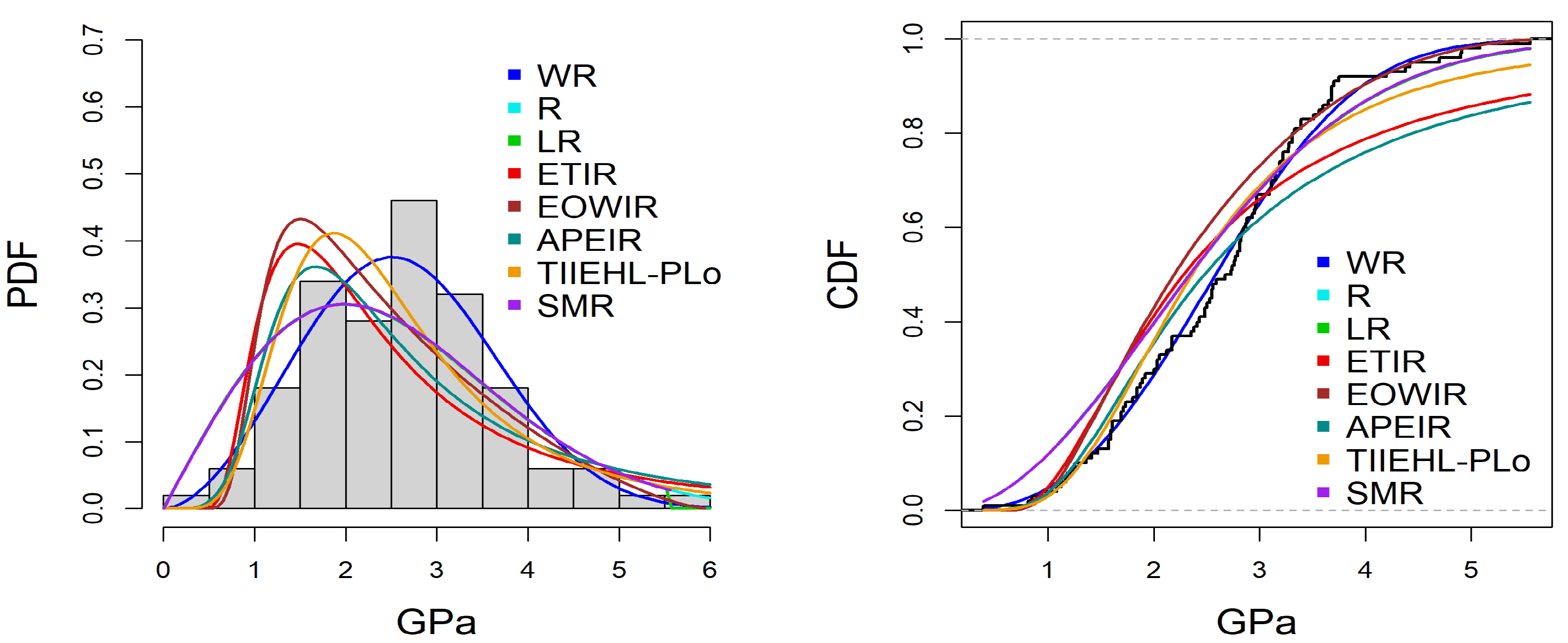
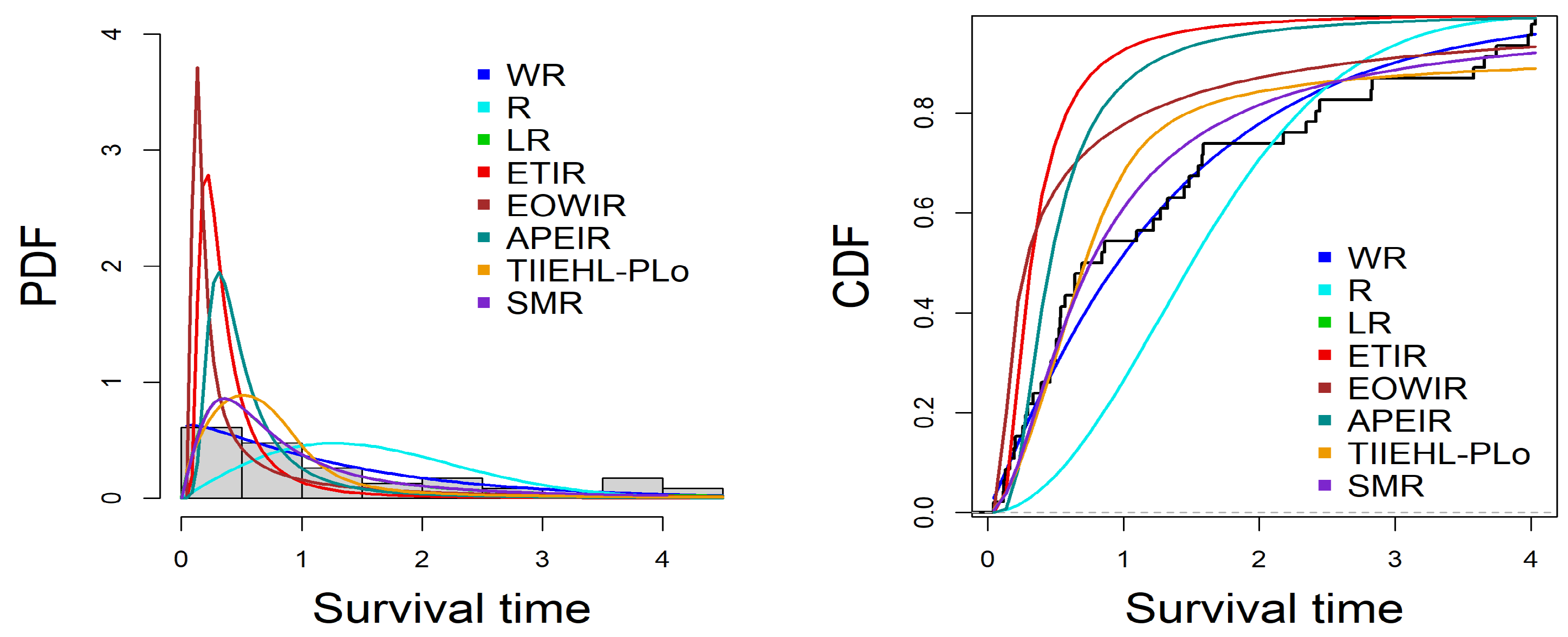
Each model’s parameters are estimated using the ML approach, and calculations are carried out using the ‘optim’ function in the R statistical program. The results are summarized in Table 6, Table 7 and Table 8, presenting the superiority of the WR model over other competing distributions in terms of goodness of fit (GoF) measures. In particular, it achieves the lowest scores in major statistics, including the Akaike Information Criterion (AIC), Bayesian Information Criterion (BIC), Consistent Akaike Information Criterion (CAIC), Hannan–Quinn Information Criterion (HQIC), Kolmogorov–Smirnov (K-S) and Anderson–Darling (A-D) tests. The K-S and A-D tests assess the alignment between the empirical distribution function of the data and the CDF of the fitted model. The null hypothesis for each test proposes that the data are in conformity with the designated distribution. As all p-values for the K-S test in Table 6, Table 7 and Table 8 exceed 0.05, we do not reject the null hypothesis. This signifies that the WR model fits the data adequately and consistently produces a larger p-value compared to competing distributions, which implies its strength in modeling the supplied datasets.
Finally, the PDF along with the CDF in all the datasets are plotted in Figure 8, Figure 9 and Figure 10 which confirms that the WR model fits the data very well, and the inherent skewness is better captured compared to other distributions.
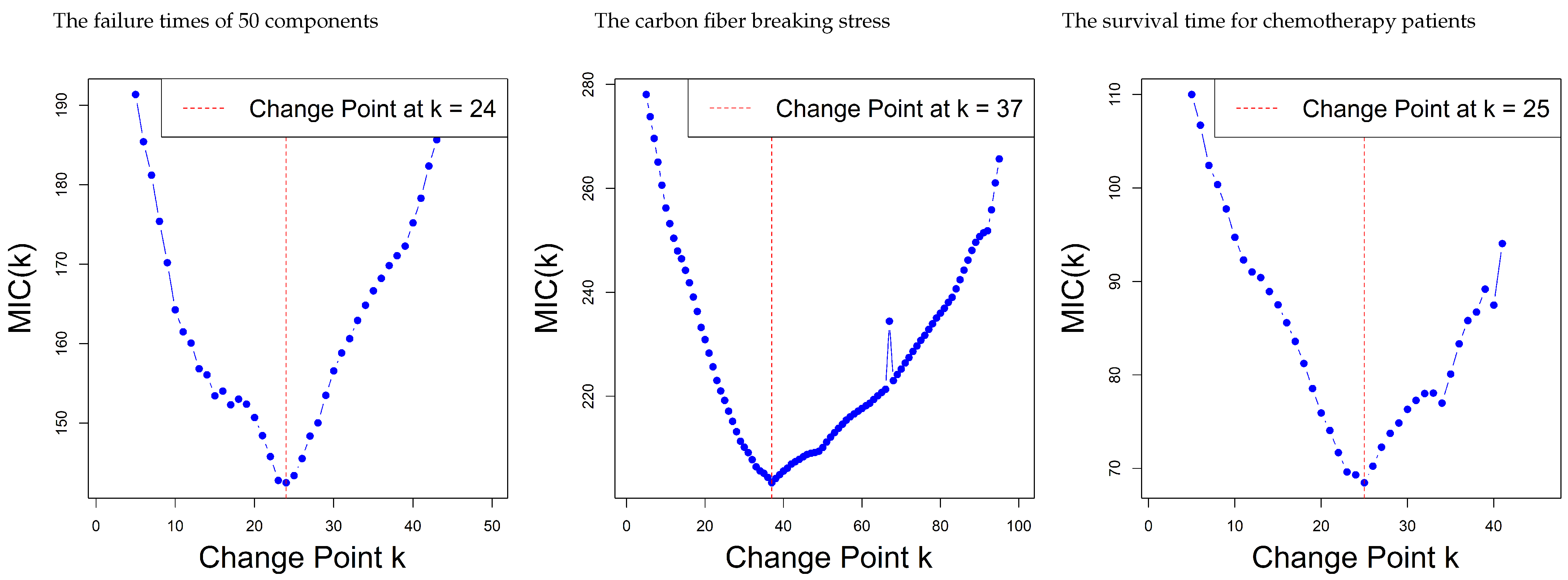
Moreover, the modified information criterion (MIC), introduced in [30], was also employed to search for potential CP in each of the real datasets using the proposed WR model. The objective of this analysis is to test whether the statistical structure of the data results in changes in a substantial way in some intervals, the fact that in such cases, it would seem more appropriate to fit two separate models (one for the before and another one for the after the CP).
The MIC is calculated as the difference in the log-likelihood of the WR distribution when the data is partitioned at a putative CP k as follows:
MIC ( k ) = 2 log L 1 ( φ ^ 1 , φ ^ n ) + 4 + 2 k n 1 2 log n ,
where L 1 ( . ) is the log-likelihood function computed independently on the two intervals, φ are the distribution parameters, and n is the overall sample size.
Under the null case (no CP), the MIC is computed over the entire dataset as:
MIC ( n ) = 2 log L 0 ( φ ^ ) + 2 log n .
It enables the detection of any meaningful transitions in the distributional structure of the data (e.g., changes in skewness, variance, or shape). A significant drop in the MIC value indicates that the three datasets before and after this point are under different statistical rules.
We present the parameter estimates for the WR distribution with and without a CP in Table 9. The results include the parameter values estimated before the CP, the parameters estimated using the complete data, and MIC criterion indices that assist in identifying the optimal CP in each dataset.
Figure 11 shows the MIC curves at each candidate point k, including the minimum value related to the estimated CP. Upon examining the results, The first example demonstrates a shift from a symmetric to a less clustered pattern, which would suggest a change in variance or shape; a second set of data shows a clear shift to the right in the skewness of the data from every well-clustered right-skewed distribution to a more smooth-like distribution which may point toward a change in experimental conditions or sample sources. The third set of series displays a change in both the concentration and the frequency of the observed effects that could reflect an external factor, such as a treatment effect or a modified measurement protocol.
These results highlight the adaptability of the proposed WR distribution in response to the underlying evolution of the data behavior, further evidencing its practical importance for real-world modeling situations.

7. Conclusions

This article proposes a new family of distributions based on the exponentiated reciprocal of the HF, called the new Weibull-G family. The Weibull–Rayleigh distribution, as one of its particular member, is extraordinarily flexible in fitting data patterns. The WR probability density function can have several shapes including symmetric, right-skewed, left-skewed, and inverse J-shaped behavior, showing its capability of fitting complicated real-world data. The HF also exhibits various shapes, such as symmetric, asymmetric, J-shaped, and inverse J-shaped, so it is well-suited for practical purposes. Important statistical measures such as quantiles, median, moments, characteristic function, order statistics, and entropy indices (Shannon and Rényi) are obtained. Five estimation methods, including MLE, PE, LSE, WLS, and CVM, are used to estimate the model parameters, and their performance is assessed through Monte Carlo simulations. The numerical results highlight the efficiency and stability of these methods. The practical potential of the WR model is evident in its superior prediction performance when applied to real datasets, outperforming traditional counterparts, which highlights its strength in modeling and interpreting complex data in various fields. In addition, the MIC was used to test for potential structural breaks in the data by comparing the fit of a single model with that of two separate models on either side of a potential break point. The MIC and its curve analysis strongly supported the CP, confirming the new model and showing how well WR explains the changes. These results demonstrate the adaptability of the proposed WR distribution in relation to the changing behavior of the data, underscoring its practical significance for real-world modeling scenarios.

Author Contributions

Conceptualization, H.B., A.S.A. and L.B.; Methodology, H.B., A.S.A. and L.B.; Software, H.A. and L.B.; Validation, H.A., A.S.A. and L.B.; Investigation, H.A. and L.B.; Data curation, H.A.; Writing—original draft, H.A.; Writing—review & editing, H.B., A.S.A. and L.B.; Visualization, H.A.; Supervision, H.B. and L.B. All authors have read and agreed to the published version of the manuscript.

Funding

This research received no external funding.

Conflicts of Interest

The authors declare no conflicts of interest.

References

  1. Alzaatreh, A.; Lee, C.; Famoye, F. A new method for generating families of continuous distributions. Metron 2013, 71, 63–79. [Google Scholar] [CrossRef]
  2. Alizadeh, M.; Cordeiro, G.M.; Pinho, L.G.B.; Ghosh, I. The Gompertz-G family of distributions. J. Stat. Theory Pract. 2017, 11, 179–207. [Google Scholar] [CrossRef]
  3. Alzaghal, A.; Famoye, F.; Lee, C. Exponentiated TX family of distributions with some applications. Int. J. Stat. Probab. 2013, 2, 31. [Google Scholar] [CrossRef]
  4. Yousof, H.M.; Alizadeh, M.; Jahanshahi, S.; Ghosh, T.G.R.I.; Hamedani, G. The transmuted Topp-Leone G family of distributions: Theory, characterizations and applications. J. Data Sci. 2017, 15, 723–740. [Google Scholar] [CrossRef]
  5. Nascimento, A.D.; Silva, K.F.; Cordeiro, G.M.; Alizadeh, M.; Yousof, H.M.; Hamedani, G.G. The odd Nadarajah-Haghighi family of distributions: Properties and applications. Stud. Sci. Math. Hung. 2019, 56, 185–210. [Google Scholar] [CrossRef]
  6. Baaqeel, H.; Alnashshri, H.; Baharith, L. A New Lomax-G Family: Properties, Estimation and Applications. Entropy 2025, 27, 125. [Google Scholar] [CrossRef] [PubMed]
  7. Alzaatreh, A.; Ghosh, I. On the Weibull-X family of distributions. J. Stat. Theory Appl. 2015, 14, 169–183. [Google Scholar] [CrossRef]
  8. Cordeiro, G.M.; M. Ortega, E.M.; Ramires, T.G. A new generalized Weibull family of distributions: Mathematical properties and applications. J. Stat. Distrib. Appl. 2015, 2, 13. [Google Scholar] [CrossRef]
  9. Najarzadegan, H.; Alamatsaz, M.H.; Hayati, S. Truncated Weibull-G more flexible and more reliable than beta-G distribution. Int. J. Stat. Probab. 2017, 6, 1–17. [Google Scholar] [CrossRef]
  10. Alizadeh, M.; Altun, E.; Afify, A.Z.; Ozel, G. The extended odd Weibull-G family: Properties and applications. Commun. Fac. Sci. Univ. Ank. Ser. A1 Math. Stat. 2018, 68, 161–186. [Google Scholar] [CrossRef]
  11. Oluyede, B.; Moakofi, T.; Chipepa, F.; Makubate, B. A new power generalized Weibull-G family of distributions: Properties and applications. J. Stat. Model. Theory Appl. 2020, 1, 167–191. [Google Scholar]
  12. Rappaport, T.S. Wireless Communications: Principles and Practice; Cambridge University Press: Cambridge, UK, 2024. [Google Scholar]
  13. Abdi, A.; Kaveh, M. K distribution: An appropriate substitute for Rayleigh-lognormal distribution in fading-shadowing wireless channels. Electron. Lett. 1998, 34, 851–852. [Google Scholar] [CrossRef]
  14. Kundu, D.; Raqab, M.Z. Generalized Rayleigh distribution: Different methods of estimations. Comput. Stat. Data Anal. 2005, 49, 187–200. [Google Scholar] [CrossRef]
  15. Alghamdi, A.; Ning, W.; Gupta, A.K. An information approach for the change point problem of the rayleigh lomax distribution. Int. J. Intell. Technol. Appl. Stat. 2018, 11, 233–254. [Google Scholar]
  16. Kilai, M.; Waititu, G.A.; Kibira, W.A.; Aldallal, R.; Bakr, M.; Tashkandy, Y.A.; Riad, F.H. Information Approach for Change Point Analysis of EGGAPE Distribution and Application to COVID-19 Data. Math. Probl. Eng. 2022, 9924902. [Google Scholar] [CrossRef]
  17. Tian, W.; Pang, L.; Tian, C.; Ning, W. Change point analysis for Kumaraswamy distribution. Mathematics 2023, 11, 553. [Google Scholar] [CrossRef]
  18. Tian, W.; Yang, Y. Change point analysis for weighted exponential distribution. Commun.-Stat.-Simul. Comput. 2024, 53, 367–379. [Google Scholar] [CrossRef]
  19. Wang, J.; Ning, W. Likelihood ratio test change point detection for the Weibull distribution with random censored data. Commun.-Stat.-Simul. Comput. 2025, 1–10. [Google Scholar] [CrossRef]
  20. R Core Team. R: A Language and Environment for Statistical Computing; R Foundation for Statistical Computing: Vienna, Austria, 2023. [Google Scholar]
  21. Aryal, G.; Elbatal, I. On the Exponentiated Generalized Modified Weibull Distribution. Commun. Stat. Appl. Methods 2015, 22, 333–348. [Google Scholar] [CrossRef]
  22. Rashwan, N.I. A note on Kumaraswamy exponentiated Rayleigh distribution. J. Stat. Theory Appl. 2016, 15, 286–295. [Google Scholar] [CrossRef]
  23. Sapkota, L.P.; Kumar, V.; Gemeay, A.M.; Bakr, M.E.; Balogun, O.S.; Muse, A.H. New Lomax-G family of distributions: Statistical properties and applications. AIP Adv. 2023, 13. [Google Scholar] [CrossRef]
  24. Venegas, O.; Iriarte, Y.A.; Astorga, J.M.; Gómez, H.W. Lomax-Rayleigh distribution with an application. Appl. Math. Inf. Sci. 2019, 13, 741–748. [Google Scholar] [CrossRef]
  25. Banerjee, P.; Bhunia, S. Exponential transformed inverse rayleigh distribution: Statistical properties and different methods of estimation. Austrian J. Stat. 2022, 51, 60–75. [Google Scholar] [CrossRef]
  26. Almetwally, E.M. Extended odd Weibull inverse Rayleigh distribution with application on carbon fibres. Math. Sci. Lett. 2021, 10, 5–14. [Google Scholar] [CrossRef]
  27. Ali, M.; Khalil, A.; Ijaz, M.; Saeed, N. Alpha-Power Exponentiated Inverse Rayleigh distribution and its applications to real and simulated data. PLoS ONE 2021, 16, e0245253. [Google Scholar] [CrossRef]
  28. Hassan, E.A.; Elgarhy, M.; Eldessouky, E.A.; Hassan, O.H.M.; Amin, E.A.; Almetwally, E.M. Different estimation methods for new probability distribution approach based on environmental and medical data. Axioms 2023, 12, 220. [Google Scholar] [CrossRef]
  29. Rivera, P.A.; Barranco-Chamorro, I.; Gallardo, D.I.; Gómez, H.W. Scale mixture of Rayleigh distribution. Mathematics 2020, 8, 1842. [Google Scholar] [CrossRef]
  30. Chen, J.; Gupta, A.K.; Gupta, A. Parametric Statistical Change Point Analysis; Birkhäuser: Boston, MA, USA, 2000; Volume 192. [Google Scholar]
Figure 1. The WR density plots for some values of α , β , θ , and λ .
Axioms 14 00649 g001
Figure 2. The WR H ( x ) plots for some values of α , β , θ and λ .
Axioms 14 00649 g002
Figure 3. Comparison of estimation techniques utilizing MSE across varying sample sizes for Table 1.
Axioms 14 00649 g003
Figure 4. Comparison of estimation techniques utilizing MSE across varying sample sizes for Table 2.
Axioms 14 00649 g004
Figure 5. Comparison of estimation techniques utilizing MSE across varying sample sizes for Table 3.
Axioms 14 00649 g005
Figure 6. Comparison of estimation techniques utilizing MSE across varying sample sizes for Table 4.
Axioms 14 00649 g006
Figure 7. Comparison of estimation techniques utilizing MSE across varying sample sizes for Table 5.
Axioms 14 00649 g007
Figure 8. Estimated PDF and CDF for the failure times of 50 components (per 1000 h).
Axioms 14 00649 g008
Figure 9. Estimated PDF and CDF for carbon fiber breaking stress (GPa).
Axioms 14 00649 g009
Figure 10. Estimated PDF and CDF for survival time for chemotherapy patients.
Axioms 14 00649 g010
Figure 11. MIC plots for identifying structural shifts in the data.
Axioms 14 00649 g011
Table 1. Simulation study at α = 4.27 , β = 0.8 , θ = 3.9 , and λ = 0.52 .
Set I: ML PE LSE WLS CVM
Est Bias MSE Est Bias MSE Est Bias MSE Est Bias MSE Est Bias MSE
α 4.53250.26250.78124.0138−0.2570.74024.2352−0.0351.11514.28240.01241.16844.58850.31851.6165
β 0.92750.12750.06670.94900.14890.07180.92730.12730.07850.92960.12960.08730.98980.18982.9075
n = 20 θ 3.90560.00560.06513.8790−0.0210.02813.8986−0.0010.08463.8914−0.0090.05283.91740.01740.1920
λ 0.5122−0.0080.00050.5102−0.0100.00040.5123−0.0080.00070.5123−0.0080.00060.5121−0.0080.0009
α 4.33840.06840.23814.0979−0.1720.29664.2009−0.0690.36294.2404−0.0300.30174.33560.06560.3844
β 0.87650.07650.01980.91120.11110.02790.88850.08850.03000.86950.09650.02830.88760.08760.0285
n = 50 θ 3.8950−0.0050.02043.8716−0.0280.00893.8946−0.0050.01773.8761−0.0240.01683.8897−0.0100.0157
λ 0.5150−0.0050.00020.5130−0.0070.00020.5136−0.0060.00020.5146−0.0050.00020.5143−0.0060.0002
α 4.28450.01450.10534.1479−0.1220.15424.2183−0.0520.17904.2423−0.0280.14884.28000.01000.1736
β 0.85510.05510.00900.88900.08890.01690.86540.06540.01250.87540.07540.01300.86680.06680.0128
n = 100 θ 3.90490.00490.00763.8667−0.0330.00483.8898−0.0100.00673.8767−0.0230.00393.8914−0.0090.0058
λ 0.5154−0.0050.00010.5149−0.0050.00010.5156−0.0040.00010.5157−0.0040.00010.5154−0.0050.0001
α 4.2534−0.0170.05444.1893−0.0810.06964.2445−0.0260.09204.2512−0.0190.07974.27600.00600.0921
β 0.85160.05160.00560.86610.06610.00800.85250.05250.00670.86700.06700.00790.85240.05240.0067
n = 200 θ 3.90830.00830.00323.8763−0.0240.00183.8890−0.0110.00283.8778−0.0220.00193.8903−0.0100.0027
λ 0.5152−0.0050.00010.5163−0.0040.00010.5165−0.0040.00000.5161−0.0040.00000.5165−0.0040.0000
α 4.2401−0.0300.03674.2023−0.0680.04974.2496−0.0200.06204.2427−0.0270.05544.2698−0.0020.0624
β 0.84540.04540.00430.86590.06590.00690.84110.04110.00500.86570.06570.00710.84250.04250.0049
n = 300 θ 3.91380.01380.00233.8779−0.0220.00143.8860−0.0140.00193.8794−0.0210.00143.8862−0.0140.0020
λ 0.5152−0.0050.00000.5161−0.0040.00000.5177−0.0020.00000.5161−0.0040.00000.5176−0.0020.0000
α 4.2366−0.0330.02334.2258−0.0440.02874.2570−0.0130.03764.2438−0.0260.03384.2696−0.0040.0380
β 0.84150.04150.00310.85890.05890.00530.83910.03910.00360.85890.05890.00550.83950.03950.0037
n = 500 θ 3.91640.01640.00183.8820−0.0180.00103.8827−0.0170.00163.8834−0.0170.00103.8828−0.0170.0016
λ 0.5154−0.0050.00000.5164−0.0040.00000.5181−0.0020.00000.5164−0.0040.00000.5181−0.0020.0000
Table 2. Simulation study at α = 5.6 , β = 2.4 , θ = 2.8 , and λ = 0.4 .
Set II: ML PE LSE WLS CVM
Est Bias MSE Est Bias MSE Est Bias MSE Est Bias MSE Est Bias MSE
α 6.04390.44391.67965.2887−0.3121.23135.5870−0.0131.95455.64930.04931.80276.05850.45853.1696
β 2.59580.19580.57262.55200.15120.51172.62390.22391.41142.63360.23361.02592.60560.20561.3017
n = 20 θ 2.82060.02060.03962.7871−0.0130.12032.82500.02500.10442.82030.02030.09462.88410.08410.1614
λ 0.3988−0.0010.00040.3951−0.0040.00080.3944−0.0060.00120.3951−0.0050.00120.3948−0.0050.0016
α 5.73250.13250.47035.4178−0.1820.46295.5402−0.0590.55665.5807−0.0190.48165.69590.09590.5785
β 2.54500.14500.19422.45450.05450.12612.52620.12620.25532.52220.12220.16692.55790.15790.2435
n = 50 θ 2.80570.00570.00822.7820−0.0180.02162.81050.01050.03052.81390.01390.02102.83070.03070.0334
λ 0.3979−0.0020.00010.3989−0.0010.00020.3960−0.0040.00050.3958−0.0040.00030.3946−0.0050.0004
α 5.65760.05760.20705.4644−0.1360.22315.5553−0.0450.29665.5973−0.0030.22535.62460.02460.2383
β 2.50210.10210.08492.42890.02890.05112.47080.07080.08932.46100.06100.07692.49600.09600.0941
n = 100 θ 2.80230.00230.00282.7903−0.0090.00862.80900.00900.01372.80330.00330.01082.82100.01200.0128
λ 0.3983−0.0020.00010.3989−0.0010.00010.3972−0.0030.00030.3986−0.0010.00010.3960−0.0040.0002
α 5.62690.02690.09965.5146−0.0850.10805.5899−0.0100.12235.60990.00990.13595.62720.02720.1274
β 2.45860.05860.04412.40380.00380.02812.43090.03090.04592.45570.05570.05842.44120.04120.0464
n = 200 θ 2.7988−0.0010.00132.80210.00210.00382.80780.00780.00552.80190.00190.00632.81380.01380.0055
λ 0.3992−0.0080.00000.3988−0.0010.00000.3985−0.0020.00100.3989−0.0010.00010.3979−0.0020.0001
α 5.61200.01200.06435.5321−0.0680.07435.5928−0.0070.08335.60020.00020.09615.61710.01710.0852
β 2.44350.04350.03282.41060.01060.02192.41220.01220.02622.43080.03080.04112.41660.01660.0287
n = 300 θ 2.7971−0.0030.00102.80540.00540.00272.80280.00280.00352.80460.00460.00442.80780.00780.0035
λ 0.3996−0.0040.00000.3983−0.0020.00000.3995−0.0050.00010.3990−0.0010.00010.39900.00100.0001
α 5.60850.00850.03805.5647−0.0350.04335.60110.00110.04735.60250.00250.06275.61480.01480.0479
β 2.43100.03100.02122.40520.00520.01462.41060.01060.01712.42650.02650.03012.41750.01750.0171
n = 500 θ 2.7968−0.0030.00062.80710.00710.00172.80120.00120.00222.80200.00200.00302.80390.00390.0022
λ 0.3999−0.0010.00000.3987−0.0010.00000.3998−0.0020.00000.39940.00060.00010.3994−0.0060.0001
Table 3. Simulation study at α = 1.39 , β = 0.32 , θ = 0.8 , and λ = 0.6 .
Set III: ML PE LSE WLS CVM
Est Bias MSE Est Bias MSE Est Bias MSE Est Bias MSE Est Bias MSE
α 1.47750.08750.01861.39200.00170.02021.43810.04810.02621.44320.05320.02311.48790.09790.0397
β 0.3094−0.0110.00200.32380.00380.00330.33010.01010.00350.32410.00410.00310.3164−0.0040.0036
n = 20 θ 0.7990−0.0010.00420.84490.04490.01250.81070.01070.00710.81220.01220.00580.7928−0.0070.0074
λ 0.5968−0.0030.00270.62070.02070.00480.61510.01510.00390.61300.01300.00320.5979−0.0020.0039
α 1.45450.06450.00851.3820−0.0080.01411.43670.04670.00931.44330.05330.00901.45190.06190.0114
β 0.3139−0.0060.00070.32040.00040.00100.32280.00280.00100.3184−0.0020.00090.3167−0.0030.0010
n = 50 θ 0.80590.00590.00190.83430.03430.00580.80870.00870.00210.81190.01190.00250.80240.00240.0021
λ 0.60860.00860.00090.61820.01820.00200.61590.01590.00150.61460.01460.00120.60820.00820.0014
α 1.44590.05590.00561.3844−0.0060.00961.43500.04500.00551.43950.04950.00501.44200.05200.0064
β 0.3152−0.0050.00030.3171−0.0030.00050.32060.00060.00060.3180−0.0020.00040.3173−0.0030.0005
n = 100 θ 0.80700.00700.00100.82670.02670.00220.80750.00750.00120.80830.00830.00090.80460.00460.0011
λ 0.61090.01090.00050.61330.01330.00100.61440.01440.00100.61350.01350.00070.61050.01050.0008
α 1.43940.04940.00381.3871−0.0030.00611.43430.04430.00381.43700.04700.00341.43720.04720.0042
β 0.3138−0.0060.00020.3163−0.0040.00030.3181−0.0020.00030.3164−0.0040.00020.3168−0.0030.0003
n = 200 θ 0.81100.01100.00060.82300.02300.00170.80670.00670.00080.80810.00810.00050.80470.00470.0008
λ 0.61160.01160.00030.61040.01040.00060.61210.01210.00060.61200.01200.00050.61000.01000.0005
α 1.43490.04490.00301.39840.00840.00401.42920.03920.00271.43170.04170.00261.42980.03980.0027
β 0.3130−0.0070.00020.3157−0.0040.00020.3172−0.0030.00020.3157−0.0040.00020.31660.00340.0002
n = 300 θ 0.81360.01360.00050.81790.01790.00100.80800.00800.00060.80960.00960.00040.80620.00620.0006
λ 0.61150.01150.00030.60990.00990.00040.61110.01110.00050.61120.01120.00040.60930.00930.0004
α 1.43180.04180.00241.40210.01210.00291.42430.03430.00191.42770.03770.00191.42510.03510.0020
β 0.3129−0.0070.00010.3162−0.0040.00010.3163−0.0040.00020.3158−0.0040.00010.3155−0.0050.0002
n = 500 θ 0.81420.01420.00040.81490.01490.00070.80890.00890.00050.80940.00940.00030.80870.00870.0005
λ 0.61110.01110.00020.60960.00960.00030.60930.00930.00030.61010.01010.00030.60840.00840.0003
Table 4. Simulation study at α = 2.5 , β = 1.8 , θ = 1.44 , and λ = 0.29 .
Set IV: ML PE LSE WLS CVM
Est Bias MSE Est Bias MSE Est Bias MSE Est Bias MSE Est Bias MSE
α 2.69120.19120.33342.3927−0.1070.24142.55180.05180.44892.57160.07160.34552.78400.28400.7107
β 1.86750.06750.20391.91140.11140.22831.88050.08050.37701.88750.08750.64041.80940.00940.3878
n = 20 θ 1.48670.04670.05801.4192−0.0210.07481.45100.01100.15531.4341−0.0060.08671.48600.04600.1021
λ 0.2861−0.0040.00140.2871−0.0030.00170.29610.00610.00360.29860.00860.00260.30080.01080.0033
α 2.56050.06050.10722.4344−0.0660.08112.51600.01600.13872.53110.03110.10572.59480.09480.1529
β 1.85650.05650.06151.87410.07410.08161.83610.03610.10571.83360.03360.08431.82300.02300.1040
n = 50 θ 1.44890.00890.01031.4122−0.0280.02231.4242−0.0160.02691.4289−0.0110.02531.4380−0.0020.0239
λ 0.2871−0.0030.00050.29050.00050.00050.29570.00570.00140.29550.00550.00120.29640.00640.0011
α 2.52360.02360.04652.4586−0.0410.03822.51160.01160.06382.51360.01360.04462.54720.04720.0661
β 1.84850.04850.02101.83710.03710.02951.82510.02510.03891.83300.03300.03441.82550.02550.0360
n = 100 θ 1.44240.00240.00271.4167−0.0230.00661.4218−0.01820.00941.4279−0.0120.00781.4290−0.0110.0088
λ 0.2870−0.0030.00020.29160.00160.00020.29510.00510.00060.29250.00250.00030.29450.00450.0005
α 2.50740.00740.01972.4759−0.0240.01702.51760.01760.02942.50900.00900.02032.53450.03450.0312
β 1.83360.03360.01021.81250.01250.00801.81780.01780.01051.83000.03000.01201.82350.02350.0120
n = 200 θ 1.44040.00040.00141.4278−0.0120.00221.4262−0.0140.00481.4326−0.0070.00281.4294−0.0110.0045
λ 0.2877−0.0020.00090.29200.00140.00010.29400.00400.00040.29040.00040.00010.29340.00340.0004
α 2.50160.00160.01292.4819−0.0180.01132.51520.01520.02112.50640.00640.01382.52700.02700.0212
β 1.82320.02320.00641.81050.01050.00651.80920.00920.00731.81340.01340.00761.81220.01220.0074
n = 300 θ 1.4397−0.0030.00091.4317−0.0080.00151.4274−0.0130.00361.4350−0.0050.00361.4294−0.0110.0036
λ 0.2884−0.0020.00010.29050.00050.00010.29410.00410.00040.29090.00090.00090.29390.00390.0003
α 2.50080.00080.00742.4943−0.0060.00632.51680.01680.01242.50220.00220.00772.52300.02300.0128
β 1.81640.01640.00461.80540.00540.00411.80090.00090.00391.80720.00720.00471.80450.00450.0038
n = 500 θ 1.4396−0.0040.00061.4356−0.0040.00081.4306−0.0090.00281.44000.00200.00101.4318−0.0080.0027
λ 0.2890−0.0010.00000.29060.00060.00000.29400.00400.00030.2899−0.0010.00010.29370.00370.0002
Table 5. Simulation study at α = 3.5 , β = 0.38 , θ = 0.28 , and λ = 0.33 .
Set V: ML PE LSE WLS CVM
Est Bias MSE Est Bias MSE Est Bias MSE Est Bias MSE Est Bias MSE
α 3.83400.33400.33213.3820−0.1180.21893.78590.28590.40543.78020.28020.31983.93880.43880.6131
β 0.47460.09460.01680.43100.05100.02710.45290.07290.01870.43910.05910.01900.44140.06140.0197
n = 20 θ 1.1963−0.0840.02001.2757−0.0040.02181.1719−0.1080.03631.1955−0.0850.03081.2042−0.0760.0291
λ 0.34400.01400.00390.34060.01060.00440.38270.05270.00900.37580.04580.00860.35880.02880.0063
α 3.68470.18470.10713.4140−0.0860.08963.68360.18360.11363.62130.12130.08913.74600.24600.1681
β 0.45920.07920.01010.39060.10660.00870.44020.06020.00810.41290.03290.00570.43480.05480.0081
n = 50 θ 1.1889−0.0910.01401.29640.13640.00731.1804−0.0990.01881.2306−0.0490.01211.1927−0.0870.0166
λ 0.34780.01780.00200.33350.00350.00180.36780.03780.00440.35150.02150.00300.35900.02900.0036
α 3.62170.12170.05003.4328−0.0670.04773.65200.15200.05693.54350.04350.04133.67190.17190.0676
β 0.45220.07220.00800.3747−0.00530.00340.43220.05220.00570.39230.01230.00310.42940.04940.0058
n = 100 θ 1.1954−0.0850.01041.30120.02120.00441.1890−0.0910.01351.2650−0.0150.00421.1980−0.0820.0120
λ 0.34460.01460.00100.33090.00850.00100.36090.03090.00260.33750.00750.00120.35490.02490.0021
α 3.58380.08380.02913.4399−0.0600.02483.63350.13350.03363.51660.01660.02123.64720.14720.0390
β 0.44210.06210.00630.3737−0.0060.00210.42670.04670.00410.38520.00520.00180.42500.04500.0041
n = 200 θ 1.2056−0.0740.00771.30440.02440.00251.1990−0.0810.01011.2787−0.0010.00171.2030−0.0770.0093
λ 0.34190.01190.00050.3266−0.0030.00040.35430.02430.00160.33120.00120.00060.35190.02190.0014
α 3.56220.06220.02033.4493−0.0510.01673.62070.12070.02543.4958−0.0040.01603.62700.12700.0274
β 0.44040.06040.00580.36970.01030.00160.42090.04090.00330.38140.00140.00140.42090.04090.0034
n = 300 θ 1.2102−0.0690.00661.30670.02670.00221.2055−0.0750.00851.28720.00720.00141.2081−0.0720.0080
λ 0.33990.00990.00030.3258−0.0040.00030.35260.02260.00130.3284−0.0020.00040.35050.02050.0011
α 3.55080.05080.01443.4535−0.0470.01113.61190.11190.02063.4810−0.0190.01033.61570.11570.0213
β 0.43700.05700.00510.3708−0.0090.00130.41950.03950.00310.3778−0.0020.00130.41970.03970.0029
n = 500 θ 1.2151−0.0650.00551.30910.02940.00201.2096−0.0700.00751.29610.01610.00141.2108−0.0690.0072
λ 0.33850.00850.00020.3233−0.0070.00030.35030.02030.00100.3256−0.0040.00030.34900.01900.0009
Table 6. GoF criteria for the failure times of 50 components (per 1000 h).
LAICBICCAICHQICK-SA-Dp-Value
WR102.3643212.7286220.3767213.6175215.64110.12700.9622 0.3646
R179.5991361.1982363.1102361.2815361.92630.448149.2520 1.116 × 10 9
LR109.6589223.3178227.1419223.5732224.77410.18302.0732 0.06138
ETIR205.0854412.1708414.0828412.2542412.89890.558670.0920 3.664 × 10 15
EOWIR112.9850231.9701237.7061232.4918234.15440.29187.2054 2.881 × 10 4
APEIR191.0954388.1908393.9269388.7126390.37520.479054.8930 4.538 × 10 11
TIIEHL PLo103.4034214.8067222.4548215.6956217.71910.133891.08860.3038
SMR109.6589223.3178227.1419223.5732224.77410.183072.07370.06133
Table 7. GoF criteria for the carbon fiber breaking stress (GPa).
LAICBICCAICHQICK-SA-Dp-Value
WR141.5293291.0586301.4793291.4797295.27600.0604830.417710.8578
R149.5009301.0018303.6070301.0426302.05620.138333.5460.04354
LR149.719303.4381308.6484303.5618305.54680.139193.59980.04153
ETIR171.0291344.0583346.6634344.0991345.11260.156745.09110.0147
EOWIR159.2529324.5058332.3213324.7558327.66880.18384.51820.002327
APEIR162.4898330.9796338.7951331.2296334.14270.189464.30.001525
TIIEHL PLo151.7267311.4533321.8740311.8744315.67080.131472.18620.06304
SMR149.5009303.0019308.2122303.1256305.11060.138483.55340.04318
Table 8. GoF criteria for the survival time for chemotherapy patients.
LAICBICCAICHQICK-SA-Dp-Value
WR58.8262125.6524132.9669126.6280128.39240.112000.56512 0.5725
R79.0742160.1484161.9770160.2393160.83340.3616814.1980 6.751 × 10 6
LR62.1893128.3786132.9959128.6577129.74870.116030.84113 0.5276
ETIR105.2395212.4791214.3077212.5700213.16410.4424427.5040 1.011 × 10 8
EOWIR78.0829162.1657167.6517162.7372164.22080.3674210.1500 4.466 × 10 6
APEIR87.8062181.6124187.0983182.1838183.66750.3375813.9590 3.526 × 10 5
TIIEHL PLo73.33895154.6779161.9925155.6535157.41800.190691.82830.06131
SMR62.18931128.3786132.9959128.6577129.74870.1160.841190.5279
Table 9. Summary of MIC analysis using the WR distribution for three data sets.
DatasetParameters Before ChangeParameters at Full DataMIC Analysis
α ^ 1 β ^ 1 θ ^ 1 λ ^ 1 α ^ n β ^ n θ ^ n λ ^ n MIC( n ) min MIC( k ) k ^
Failure times of 50 components0.88171.64120.87210.62511.09561.74830.51810.4486212.5527142.501424
Carbon fiber breaking stress3.256512.02351.16510.57123.0071.46134.71520.2517292.2689203.376737
Survival time for chemotherapy patients0.79651.99690.98520.33711.20541.87511.13950.2142125.309668.466525
Disclaimer/Publisher’s Note: The statements, opinions and data contained in all publications are solely those of the individual author(s) and contributor(s) and not of MDPI and/or the editor(s). MDPI and/or the editor(s) disclaim responsibility for any injury to people or property resulting from any ideas, methods, instructions or products referred to in the content.