Article

Inference for Maximum Ranked Set Sampling with Unequal Samples from the Burr Type-III Model with Cycle Effects

1
School of Mathematics, Yunnan Normal University, Kunming 650500, China
2
Yunnan Key Laboratory of Modern Analytical Mathematics and Applications, Yunnan Normal University, Kunming 650500, China
3
Department of Mathematics, Indian Institute of Technology Patna, Bihta 801106, India
4
Department of Mathematical Sciences, University of South Dakota, Vermillion, SD 57069, USA
*
Author to whom correspondence should be addressed.
Axioms 2025, 14(8), 619; https://doi.org/10.3390/axioms14080619
Submission received: 7 July 2025 / Revised: 31 July 2025 / Accepted: 4 August 2025 / Published: 8 August 2025

Abstract

This paper explores statistical inferences for the maximum ranked set sampling with unequal samples (MaxRSSU) from the Burr Type-III distribution. Under the assumption that the differences between different multiple MaxRSSU cycles are non-ignorable, classical likelihood and Bayesian approaches are employed for estimation of the model parameters and reliability indices. By taking into account the multiple-cycle effect, the maximum likelihood estimators for the parameters of the Burr Type-III distribution are established, along with an analysis of their existence and uniqueness. Furthermore, approximate confidence intervals are constructed based on asymptotic theory. In addition, a hierarchical Bayesian framework is conducted for analysis, and a Monte Carlo sampling method is proposed for complex posterior computation. Extensive simulation studies are carried out for evaluating the performance of the proposed methods, and a further two real-data examples are also provided for illustration. The numerical results indicate that the proposed methods work satisfactorily and the hierarchical Bayesian approach appears more appealing when the uncertainty cycle effect is involved.

1. Introduction

In practice, the reliability evaluation of units or systems predominantly employs lifespan data collected in various situations and experimental schemes, and obtaining complete data from simple random sampling (SRS) is the traditional approach used in data analysis. Although SRS retains notable and appealing advantages in statistical inference, such as unbiased population representation and a well-established theoretical framework, its practical implementation in reliability testing faces significant challenges in practical engineering contexts. For example, the SRS method frequently requires extensive sample sizes and incurs prohibitive cost and time burdens, particularly when dealing with high-value or low-failure-rate products. Due to these time and cost constraints from SRS, various sampling frameworks have been developed, with one of the most popular schemes being ranked set sampling (RSS). It has emerged as a viable alternative to SRS and strategically incorporates expert judgment into the sampling process. In addition, RSS also effectively addresses some critical constraints of the traditional SRS approach for lifespan data collection. In particular, RSS achieves an estimation accuracy comparable to that of SRS with fewer experimental units and significantly reduces the testing costs for high-failure-cost products. Similarly, through cycle ranking and systematic selection, RSS inherently stratifies population heterogeneity, thereby enhancing detection capability for latent failure patterns that SRS might overlook in complex systems.
The traditional RSS framework was introduced by McIntyre [1] to determine the mean pasture population, and its high efficiency was demonstrated by various authors by comparing it with traditional SRS from different perspectives. For example, Bouza [2] used RSS and randomized response techniques to estimate the mean of a sensitive quantitative characteristic. It was found that the use of RSS is highly beneficial and leads to estimators which are more precise than for SRS data. He et al. [3] investigated the maximum likelihood estimation of the log-logistic distribution under both SRS and RSS frameworks. The results revealed the superior performance of the RSS-based method over that of SRS, particularly under imperfect ranking conditions. Similar work has also been undertaken by Taconeli [4], Nawaz [5], Qian [6] and Dumbgen [7] (see also the references therein). Generally, the RSS framework can be described as follows. Suppose that there are n 2 identical units randomly selected from the population; then, n groups of size n in each group are further defined based on these n 2 units. In each group, units are ranked according to straightforward and inexpensive ranking criterion, such as expert judgment, visual inspection, or use of auxiliary variables, without measuring them. In such a scenario, the unit ranked lowest is chosen for actual quantification from the first group of n units, while the unit ranked second lowest is measured from the second group of n. The process is continued until the unit ranked highest is measured from the n-th set of size n. The data { X ( 1 ) 1 , X ( 2 ) 2 , , X ( n ) n } are called the RSS observation of size n, where the notation X ( j ) s denotes the j-th order statistic in the s-th set for s , j = 1 , 2 , , n . For a visual presentation, the traditional RSS framework is described as follows:
Set Ranking RSS 1 X ( 1 ) 1 X ( 2 ) 1 X ( n ) 1 X ( 1 ) 1 2 X ( 1 ) 2 X ( 2 ) 2 X ( n ) 2 X ( 2 ) 2 n X ( 1 ) n X ( 2 ) n X ( n ) n X ( n ) n
Although traditional RSS has demonstrated advantages in improving statistical efficiency and reducing costs compared to SRS, its reliance on balanced sample sizes and structured ranking assumptions may limit its applicability under certain conditions. Due to these practical and theoretical limitations, numerous modified RSS strategies have been developed to address the constraints. These include extreme RSS ([8]), mean ranked sampling ([9]), quartile RSS ([10]), paired RSS ([11]), multistage RSS ([12]), and stratified pair RSS ([13]), among others. Each of these strategies offers unique advantages for different study designs and data characteristics. Among the different RSS frameworks, one popular modified RSS approach, called maximum ranked set sampling with unequal samples (MaxRSSU), introduced by Bhoj [14], has attracted much attention in the literature. It modifies the sampling procedure to account for unequal samples, leading to a significant improvement in sampling efficiency and estimation accuracy in certain scenarios. In the context of MaxRSSU, the procedure is structured as follows. There are n ( n + 1 ) 2 identical units selected from the population which are randomly divided into n groups of sizes 1 , 2 , , n y. Then, the highest rank unit is chosen for the actual quantification of the i-th group of size i with i = 1 , 2 , , n . Therefore, sample { X ( 1 ) 1 , X ( 2 ) 2 , , X ( n ) n } is called the MaxRSSU observation of size n in this scenario. For illustration, the MaxRSSU scheme is described as follows:
Set Ranking MaxRSSU 1 X ( 1 ) 1 X ( 1 ) 1 2 X ( 1 ) 2 X ( 2 ) 2 X ( 2 ) 2 n X ( 1 ) n X ( 2 ) n X ( n ) n X ( n ) n
The MaxRSSU procedure has several advantages compared to traditional RSS. For example, the MaxRSSU approach accommodates unequal sample sizes across subgroups, allowing adaptive resource allocation. This is useful in field studies where logistical constraints or costs limit equal-sized sampling. Consequently, unequal sample sizes in this case also allow strategic allocation of measurement efforts, optimizing time and resource usage while maintaining precision. In addition, by prioritizing maximum ranks, MaxRSSU can better capture extreme values, making it ideal for environmental monitoring, epidemiology, or quality control where outliers are of primary interest. Due to its great flexibility and potential advantages, the MaxRSSU approach has received considerable attention and been discussed by many authors (see, for example, the contributions of Eskandarzadeh et al. [15], Qiu et al. [16], and Basikhasteh et al. [17], among others).
The above scenarios are called single-cycle RSS frameworks; however, in practical applications, such single-cycle RSS frameworks are often extended to multiple-cycle RSS to address complexities arising from population heterogeneity, resource constraints, or measurement limitations. This hierarchical approach involves iteratively applying ranking and selection procedures across sequential phases, thereby balancing statistical efficiency with operational feasibility. In addition, this approach is particularly valuable in large-scale surveys involving geographically dispersed populations. The multiple-cycle strategy not only reduces logistical burdens but also enhances the representativeness of the sample when subpopulations exhibit distinct characteristics. Under the MaxRSSU framework with a k-cycle design, the corresponding multiple-stage MaxRSSU scenario can be described as follows:
Cycle       1       2       k Ranking X ( 1 ) 1 1 X ( 1 ) 2 1 X ( 2 ) 2 1 X ( 1 ) n 1 1 X ( 2 ) n 1 1 X ( n 1 ) n 1 1 X ( 1 ) 1 2 X ( 1 ) 2 2 X ( 2 ) 2 2 X ( 1 ) n 2 2 X ( 2 ) n 2 2 X ( n 2 ) n 2 2 X ( 1 ) 1 k X ( 1 ) 2 k X ( 2 ) 2 k X ( 1 ) n k k X ( 2 ) n k k X ( n k ) n k k MaxRSSU { X ( 1 ) 1 1 , X ( 2 ) 2 1 , , X ( n 1 ) n 1 1 } { X ( 1 ) 1 2 , X ( 2 ) 2 2 , , X ( n 2 ) n 2 2 } { X ( 1 ) 1 k , X ( 2 ) 2 k , , X ( n k ) n k k }
where the notation X ( j ) s i denotes the j-th ( j = 1 , 2 , , n i ) ranked observation in ascending order from the s-th group ( s = 1 , 2 , , n i ) in the i-th MaxRSSU cycle with i = 1 , 2 , , k . To simplify notation, MaxRSSU samples drawn from the i-th cycle are denoted as X i 1 , X i 2 , , X i n i . It is noted that the multiple-cycle MaxRSSU framework is applied through sequential sampling phases in a MaxRSSU scenario. Similarly, there are also various cases where the multiple-cycle scenario has been adopted for other RSS schemes. For example, see Wolfe [18], Wang [19], Taconeli [4] and Akdeniz [20], as well as the references therein.
In practical experimental designs, multiple-cycle RSS is widely adopted for its efficiency in improving estimation accuracy by leveraging stratification within each cycle. However, when extending RSS to multiple-cycle settings for longitudinal or large-scale product evaluations, differences between different cycles (DBDC) emerge as critical sources of bias due to inherent experimental limitations. Specifically, factors such as instrument drift over time, technician-dependent sorting inconsistencies, or shifts in operational protocols across cycles (e.g., modifications in subgroup ranking criteria or uneven allocation of sample units) can disrupt the comparability of rankings and measurements between cycles. These cyclical discrepancies directly violate the assumption of statistical homogeneity commonly imposed in multiple-cycle RSS analyses, making conventional methods—which often pool data across cycles as if they were interchangeable—prone to severe inaccuracies. For example, unaccounted for drift in measurement tools might introduce spurious trends in ranked data, while protocol variations could distort comparison of product performance between cycles. Such biases could lead to misleading inferential outcomes, such as overestimating treatment effects, inflating type I errors, or masking true variability due to the conflation of experimental noise and genuine product-related signals. Therefore, explicitly modeling the effects of DBDC in multiple-cycle RSS frameworks becomes imperative to preserve the integrity of statistical conclusions, ensure robust estimation, and enable valid comparisons across experimental cycles. Therefore, it is necessary to take the DBDC into account in data analysis, otherwise ignoring inter-group variability maybe lead to biased and inaccurate results (see, for example, some recent contributions of Ahmadi et al. [21], Zhu [22], Kumari et al. [23], Wang et al. [24], as well as references therein). Motivated by the aforementioned reasons and due to the potential applications of the multiple-cycle MaxRSSU framework, this paper is devoted to the discussion of statistical inference of multiple-cycle MaxRSSU data from the Burr Type-III (BIII) population when the DBDC is taken into account.
Given the potential benefits of incorporating cycle effects in improving the flexibility and design of experimental studies, this paper investigates the statistical inference challenges associated with using the BIII distribution for equipment lifetime analysis under MaxRSSU. The main contributions of this study are summarized as follows. Firstly, by applying maximum likelihood estimation (MLE) to the parameters of the multiple-cycle BIII model, we establish the theoretical conditions for the existence and uniqueness of these parameters. This provides a solid foundation for improving the numerical stability and computational performance of likelihood-based methods. Secondly, to more accurately capture the cycle effects, we propose an enhanced hierarchical Bayesian model for statistical inference. By integrating historical data or expert knowledge into the inference framework, the hierarchical Bayesian approach offers notable advantages over traditional frequentist methods in terms of both flexibility and estimation accuracy. Thirdly, this paper has certain practical value in the field of engineering management. We provide engineers and technicians with an alternative multiple-cycle life testing scheme that offers greater flexibility. At the same time, we also propose a more efficient statistical inference method, which can be used to effectively analyze the reliability of equipment or systems under conditions of limited cost and time, where sample sizes are relatively small.
The article is structured as follows. Section 2 provides a description of the population model and outlines multiple-cycle MaxRSSU data and the associated likelihood function. Section 3 presents the classical estimation of unknown parameters and the reliability indices. The hierarchical Bayesian model is described in Section 4. In Section 5, the likelihood ratio test is examined. Numerical studies and two real-life examples are explored in Section 6. Finally, Section 7 provides concluding remarks.

2. Model Description and Likelihood Function

In this section, a population model of MaxRSSU data is provided and a data description is also provided in the context of a multiple-cycle MaxRSSU scenario.

2.1. Burr Type-III Model

Suppose that the random variable X follows the BIII distribution with cumulative distribution function (CDF) and the probability density function (PDF) as follows:
F ( x ; c , θ ) = ( 1 + x c ) θ and f ( x ; c , θ ) = θ c x ( c + 1 ) ( 1 + x c ) ( θ + 1 ) , x > 0 ,
where θ > 0 and c > 0 are scale and shape parameters, respectively. Consequently, the survival function (SF) and the hazard rate function (HRF) of the BIII model can be expressed at mission time t as
S ( t ) = 1 ( 1 + t c ) θ and h ( t ) = θ c t ( c + 1 ) ( 1 + t c ) ( θ + 1 ) 1 ( 1 + t c ) θ .
In addition, since the mean time to failure of the BIII model has no closed form, an alternative reliability index called the median time to failure (MdTF) is given by
MdTF = ( 2 1 / θ 1 ) 1 c .
It is observed that the BIII model incorporates two shape parameters, which enable it to flexibly capture the characteristics and tendencies of diverse datasets. This inherent flexibility enhances its fitting performance, making it a highly adaptable tool in data analysis (for further research on the BIII distribution, please refer to the studies by Kim et al. [25], Cordeiro [26], and Domma et al. [27]). In addition, this model is treated as an alternative to the traditional Weibull, gamma, and log-normal distributions, and has been widely used in various practical fields, such as finance, environmental studies, survival analysis, and reliability theory. For example, some recent contributions have been provided by Singh et al. [28], Omea et al. [29], and Feroze et al. [30]. For illustration, several plots of the PDF and HRF are presented in Figure 1 using various parameter values, demonstrating the model’s considerable flexibility in fitting data.

2.2. Data Description and Likelihood Function

Consider a multiple-cycle MaxRSSU scenario with k groups for identical units from the BIII distribution, and n i MaxRSSU data are observed in the i-th ( i = 1 , 2 , , k ) cycle, with each cycle. Given the premise that the units from each cycle adhere to a consistent failure mechanism, it is assumed that a unified model coupled with a shared parameter is employed to underscore their inherent similarities. In addition, to account for the variability in DBDC across k groups, distinct parameters are introduced for each cycle to capture the unique characteristics inherent to the respective settings. This approach not only provides a more accurate representation of common failure properties but also effectively addresses the heterogeneity arising from diverse cycle environments. Within the context of the MaxRSSU scenario, the following observations and associated distributions are assumed:
Cycle Data Samples Distribution 1 D 1 ( x 11 , x 12 , , x 1 n 1 ) BIII ( c , θ 1 ) 2 D 2 ( x 21 , x 22 , , x 2 n 2 ) BIII ( c , θ 2 ) k D k ( x k 1 , x k 2 , , x k n k ) BIII ( c , θ k )
where the parameters θ 1 , θ 2 , , θ k are distinct parameters reflecting the DBDC effect among the k MaxRSSU cycles.
From (4), the likelihood function of ( c , θ i ) with data D i , i = 1 , 2 , , k under the i-th cycle is given by
L i ( c , θ i ; D i ) j = 1 n i j f ( x i j ; c , θ i ) [ F ( x i j ; c , θ i ) ] j 1 .
Further, let D = ( D 1 , D 2 , , D k ) and Θ = ( θ 1 , θ 2 , , θ k ) . The full likelihood function of c and Θ can be expressed as
L ( c , Θ ; D ) i = 1 k L i ( c , θ i , D i ) = i = 1 k j = 1 n i j θ i c x i j ( c + 1 ) ( 1 + x i j c ) ( j θ i + 1 ) .
In addition, under the assumption that the DBDC effect among multiple MaxRSSU cycles is nonignorable, the parameter θ can be obtained by weighted estimation of θ i , i = 1 , 2 , , k as θ = i = 1 k ω i θ i i = 1 k ω i , where ω i , i = 1 , 2 , , k is the weight coefficient, discussed below.

3. Classical Estimation

In this section, the MLEs of the model parameters, SF, HRF as well as MdTF are developed. Following this, approximate confidence intervals (ACIs) are also constructed.

3.1. Maximum Likelihood Estimation

From (6), the associated log-likelihood function of c and Θ can be obtained as
( c , Θ ; D ) i = 1 k n i ln ( c θ i ) ( c + 1 ) i = 1 k j = 1 n i ln x i j i = 1 k j = 1 n i ( j θ i + 1 ) ln ( 1 + x i j c ) .
By taking the derivatives of ( c , Θ ; D ) with respect to θ 1 , θ 2 , , θ k and c, the MLEs for θ ^ 1 , θ ^ 2 , , θ ^ k and c ^ can be obtained through the following likelihood equation:
( c , Θ ; D ) θ i = 0 , i = 1 , 2 , , k and ( c , Θ ; D ) c = 0 .
However, it is seen that there are not closed forms for the associated MLEs of the model parameters and that a convergence problem may also exist in the numerical approach for finding the estimates using the nonlinear equations. An alternative profile likelihood approach is employed here, where the estimators that maximize the profile likelihood function are also the MLEs obtained from the full likelihood function. For more details, see the monograph by Barndorff-Nielsen and Cox [31].
Theorem 1.
For given c and n i > 0 , i = 1 , 2 , , k , the MLE θ ˜ i of parameter θ i is obtained as follows:
θ ˜ i = n i j = 1 n i j ln ( 1 + x i j c ) , i = 1 , 2 , , k .
Proof. 
By taking the derivatives of ( c , Θ ; D ) and setting them to zero, one can obtain θ ^ i directly. Moreover, using the inequality ln θ i θ ˜ i θ i θ ˜ i 1 ( θ i θ ˜ i > 0 ) , i = 1 , 2 , , k , one has
ln θ i ln θ ^ i 1 + θ i n i j = 1 n i j ln ( 1 + x i j c ) , i = 1 , 2 , , k .
Ignoring the constant terms and using (7) and (9), the following result is obtained:
( c , Θ ; D ) i = 1 k n i ln ( c θ ˜ i ) ( c + 1 ) i = 1 k j = 1 n i ln x i j i = 1 k j = 1 n i ln ( 1 + x i j c ) i = 1 k n i .
Since n i = θ ˜ i j = 1 n i j ln ( 1 + x i j c ) , i = 1 , 2 , , k , it is noted that
( c , Θ ; D ) i = 1 k n i ln ( c θ ˜ i ) ( c + 1 ) i = 1 k j = 1 n i ln x i j i = 1 k j = 1 n i ( j θ ˜ i + 1 ) ln ( 1 + x i j c ) = ( c , Θ ˜ ; D ) ,
where the equality holds if, and only if, θ i = θ ˜ i , i = 1 , 2 , , k . Therefore, the assertion is fulfilled. □
Using Theorem 1 and ignoring the constant terms, the profile log-likelihood of c can be obtained by substituting θ i with θ ˜ i in (7) as
( c ; D ) i = 1 k n i ln c i = 1 k n i ln j = 1 n i j ln ( 1 + x i j c ) c i = 1 k j = 1 n i ln x i j i = 1 k j = 1 n i ln ( 1 + x i j c ) .
Theorem 2.
The MLE c ^ exists as the unique solution of the following equation. Then, the likelihood function of parameter c is conducted as
Φ ( c ) = i = 1 k n i c i = 1 k j = 1 n i ln ( x i j ) 1 + x i j c + i = 1 k n i j = 1 n i j x i j c ln ( x i j ) 1 + x i j c j = 1 n i j ln ( 1 + x i j c ) = 0 .
Proof. 
By taking the derivative of the profile log-likelihood function ( c ; D ) in (10), then the likelihood function of parameter c is conducted directly, and it is also noted that the function Φ ( c ) can be rewritten alternatively as
Φ ( c ) = i = 1 k Φ i ( c ) and Φ i ( c ) = n i c j = 1 n i ln ( x i j ) 1 + x i j c + n i j = 1 n i j x i j c ln ( x i j ) 1 + x i j c j = 1 n i j ln ( 1 + x i j c ) , i = 1 , 2 , , k .
Consequently, it is noted that lim c 0 Φ i ( c ) = + , lim c Φ i ( c ) < 0 and Φ i ( c ) < 0 for i = 1 , 2 , , k ; then, one has that the function Φ ( c ) monotonically decreases continuously from positive to negative with respect to the parameter c, indicating that the equation Φ ( c ) = 0 has a unique solution with respect to c. Therefore, the existence and uniqueness of the MLE c ^ hold (see also the works of Wingo [32], and Singh [33]). Therefore, the assertion is fulfilled. □
Clearly, it is not possible to find the MLE c ^ from (11) with a closed form. In consequence, a fixed-point numerical iterative approach, namely, Algorithm 1 is adopted to find the solution of the MLE c ^ . Consequently, the MLE of θ i , i = 1 , 2 , , k can be obtained from Theorem 1 as
θ ^ i = n i j = 1 n i j ln ( 1 + x i j c ^ ) , i = 1 , 2 , , k .
Algorithm 1: Iterative method for finding MLE c ^ .
Step 1 
An initial guessed value of parameter c ( 0 ) of c is given with k = 0 .
Step 2 
To solve for the function Ψ ( c ) in terms of c, set Φ ( c ) = 0 , Ψ ( c ) is defined as
Ψ ( c ) = i = 1 k n i i = 1 k j = 1 n i ln x i j i = 1 k j = 1 n i j n i + 1 x i j c ln x i j 1 + x i j c .
Step 3 
Compute c ( k + 1 ) = Ψ ( c ( k ) ) .
Step 4 
Set k = k + 1 .
Step 5 
For a given accuracy level ε , the iterative procedure stops if c ( k + 1 ) c ( k ) ε ; else repeat Steps 3 and 4 until convergence.
Furthermore, leveraging the invariance property of maximum likelihood estimation, the MLEs of the stress characteristics, such as SF, HRF, and MdTF, can also be estimated as
R ^ ( t ; c , θ ) = R ( t ; c ^ , θ ^ ) , h ^ ( t ; c , θ ) = h ( t ; c ^ , θ ^ ) , MdTF ^ ( c , θ ) = MdTF ( c ^ , θ ^ ) ,
where the notation θ ^ is the MLE of the population parameter θ that is estimated as
θ ^ = i = 1 k ω ^ i θ ^ i i = 1 k ω ^ i ,
with ω ^ i = 1 / var ( θ ^ i ) serving as the estimator of the coefficient ω i for i = 1 , 2 , , k . Additionally, var ( θ ^ i ) represents the observed variance of the estimate of θ i under the i-th cycle, details of which are reported below.

3.2. Approximate Confidence Intervals

Since the MLEs of the model parameters do not have a closed-form solution, exact confidence intervals for the parameters and survival characteristics cannot be obtained. Consequently, large-sample approximation theory and the delta method are employed to derive the corresponding ACIs in this part.
Suppose v = ( θ 1 , θ 2 , , θ k , c ) with v i = θ i , i = 1 , 2 , , k , and v k + 1 = c . By differentiating Equation (7) twice with respect to the parameter θ 1 , θ 2 , , θ k , c , the second derivatives of ( v ) = ( θ 1 , θ 2 , , θ k , c ) can be obtained as
2 θ i 2 = n i θ i 2 , 2 θ i c = 2 c θ i = j = 1 n i j x i j c ln x i j 1 + x i j c ,
2 c 2 = i = 1 k n i c 2 + i = 1 k j = 1 n i ( j θ i + 1 ) ( ln x i j ) 2 x i j c ( 1 + x i j c ) 2 .
and
2 θ i θ j = 0 , i , j = 1 , 2 , , k .
Therefore, the observed Fisher information matrix, namely, I ( v ) can be written as
I ( v ^ ) = I 11 I 12 I 1 ( k + 1 ) I 21 I 22 I 2 ( k + 1 ) I k 1 I k 2 I k ( k + 1 ) I ( k + 1 ) 1 I ( k + 1 ) 2 I ( k + 1 ) ( k + 1 ) v = v ^ ,
where notation I i j = 2 v i v j , i , j = 1 , 2 , , k + 1 and v ^ = ( θ ^ 1 , θ ^ 2 , , θ ^ k , c ^ ) .
Theorem 3.
Under mild regularity conditions, the asymptotic distribution of MLE v ^ is
( v ^ v ) N 0 , I 1 ( v ^ ) ,
where I 1 ( v ^ ) is the inverse of the observed Fisher information matrix given by
I 1 ( v ^ ) = var ( θ ^ 1 ) cov ( θ ^ 1 , θ ^ 2 ) cov ( θ ^ 1 , c ^ ) cov ( θ ^ 2 , θ ^ 1 ) var ( θ ^ 2 ) cov ( θ ^ 2 , c ^ ) cov ( θ ^ k , θ ^ 1 ) cov ( θ ^ k , θ ^ 2 ) cov ( θ ^ k , c ^ ) cov ( c ^ , θ ^ k ) cov ( c ^ , θ ^ k ) var ( c ^ ) .
Proof. 
Using the multivariate asymptotic normality of the MLE, the result can be established directly. □
For arbitrary 0 < γ < 1 , 100 ( 1 γ ) % ACI of θ i ( i = 1 , 2 , , k ) and c can be constructed as
θ ^ i z γ / 2 var ( θ ^ i ) , θ ^ i + z γ / 2 var ( θ ^ i ) ,
and
c ^ z γ / 2 var ( c ^ ) , c ^ + z γ / 2 var ( c ^ ) ,
where z γ is the upper 100 γ % percentile of a standard normal distribution.
Furthermore, to determine the confidence intervals for the associated parameters and reliability indices, such as θ , R ( t ; c , θ ) , h ( t ; c , θ ) and MdTF, the following asymptotic normality result is established for this purpose.
Theorem 4.
Let g ( v ) be an arbitrary continuous function of parameter v , and g ^ ( v ) = g ( v ^ ) be the MLE of g ( v ) , then
g ^ ( v ) g ( v ) N 0 , var ( g ^ ( v ) ) ,
where notation var ( g ^ ( v ) ) is the asymptotic variance of MLE g ^ ( v ) given by
var ( g ^ ( v ) ) = g ( v ^ ) I 1 ( v ^ ) g ( v ^ ) ,
with
g ( v ^ ) = g ( v ) v 1 , g ( v ) v 2 , , g ( v ) v k , g ( v ) v k + 1 v = v ^ .
Proof. 
Using Theorem 3 and applying the delta method, the asymptotic distribution of g ( v ) can be derived. For the sake of conciseness, the detailed steps are omitted. □
Therefore, the asymptotic distribution of g ^ ( v ) = g ( v ^ ) is given by g ^ ( v ) g ( v ) var ( g ^ ) N 0 , 1 , and then the 100 ( 1 γ ) % ACI of g ( v ) can be constructed as
( g ^ ( v ) z γ / 2 var ( g ^ ) , g ^ ( v ) + z γ / 2 var ( g ^ ) ) .
Let g ( v ) represent the associated parameters and reliability indices. The ACIs can then be derived accordingly, with the detailed steps omitted for brevity.

4. Hierarchical Bayesian Estimation

In this section, a hierarchical model along with Bayes inference is proposed to estimate the model parameters and reliability indices.

4.1. Hierarchical Priors

In the hierarchical framework, it is assumed that an independent gamma prior is assigned to each parameter θ i , i = 1 , 2 , , k , reflecting the independent testing mechanisms across multiple facilities with cycle effects. Consequently, the joint prior for Θ can be expressed as follows:
π ( Θ | α , β ) i = 1 k θ i α 1 e β θ i , α > 0 , β > 0 ,
where α and β are hyper-parameters. Moreover, the hyper-parameters α and β in the second stage are further assumed to have a non-information prior as
π ( α , β ) 1 , α > 0 , β > 0 .
In addition, an independent non-information prior for parameter c is considered as
π ( c ) 1 , c > 0 .
Therefore, the full posterior density of Λ = ( θ 1 , , θ k , c , α , β ) is given by
π ( Λ D ) π ( c ) π ( α , β ) π ( Θ ) L ( c , Θ ; D ) i = 1 k θ i α 1 e β θ i × i = 1 k j = 1 n i j θ i c x i j ( c + 1 ) ( 1 + x i j c ) ( j θ i + 1 ) .
Let η ( Λ ) be an arbitrary continuous function of parameter Λ = ( θ 1 , , θ k , c , α , β ) , such as the model parameters, SF, HRF and MdTF, then the corresponding Bayes estimator of η ( Λ ) under squared error loss can be obtained as
η ^ ( Λ ) = E ( η ( Λ ) | D ) = 0 η ( Λ ) π ( c ) π ( α , β ) π ( Θ ) L ( c , Θ ; D ) d Λ 0 π ( c ) π ( α , β ) π ( Θ ) L ( c , Θ ; D ) d Λ ,
where notation 0 [ · ] d Λ = 0 0 [ · ] d θ 1 d θ k d c d α d β . Clearly, obtaining the Bayes estimator η ^ ( Λ ) from Equation (20) analytically is a challenge. Therefore, a Monte Carlo sampling method is employed to compute the Bayes estimate as an alternative approach. Within the hierarchical framework, a Metropolis–Hastings (MH) algorithm is proposed for this purpose in conjunction with Gibbs sampling.

4.2. Bayesian Posterior Computation

From (19), the conditional posterior densities of θ i , i = 1 , 2 , , k can be expressed as
π ( θ i c , α , β , D ) θ i α + n i 1 exp j = 1 n i ( j θ i + 1 ) ln ( 1 + x i j c ) β θ i , θ i > 0 , i = 1 , 2 , , k ,
and the conditional posterior density of α and β are given by
π ( α Θ , c , β , D ) i = 1 k θ i α 1 , α > 0 ,
π ( β Θ , c , α , D ) exp β i = 1 k θ i , β > 0 ,
and the conditional posterior density of c can be expressed as
π ( c Θ , α , β , D ) c i = 1 k n i i = 1 k j = 1 n i x i j c ( 1 + x i j c ) ( j θ i + 1 ) , c > 0 .
It is observed that, except for the posterior π ( β Θ , c , α , D ) in Equation (), which follows an exponential distribution, the other conditional posterior densities given in Equations (21), (22), and (24) do not simplify to well-known distributions. Therefore, a Gibbs sampling approach combined with the MH method, referred to as Algorithm 2, is proposed to construct Bayes estimates and credible intervals associated with the highest posterior density (HPD) within the hierarchical framework.
Algorithm 2: Sampling approach for the Bayes estimation.
Step 1 
Start with initial values Λ ( 0 ) = Θ ( 0 ) , c ( 0 ) , α ( 0 ) , β ( 0 ) with Θ ( 0 ) = θ 1 ( 0 ) , θ 2 ( 0 ) , , θ k ( 0 ) .
Step 2 
Set s = 1.
Step 3 
Generate c ( s ) from π ( c ( s 1 ) Θ ( s 1 ) , α ( s 1 ) , β ( s 1 ) , D ) with normal proposal N c ( s 1 ) , var ( c ) using MH sampling as follows
(i) 
Generate c from N c ( s 1 ) , var ( c ) with var ( c ) from the variances-covariance matrix.
(ii) 
Calculate p = min 1 , π ( c Θ ( s 1 ) , α ( s 1 ) , β ( s 1 ) , D ) π ( c ( s 1 ) Θ ( s 1 ) , α ( s 1 ) , β ( s 1 ) , D ) and generate u U ( 0 , 1 ) .
(iii) 
If u p , then accept c ( s ) = c , otherwise c ( s ) = c ( s 1 ) .
Step 4 
Generate θ i ( s ) , i = 1 , 2 , , k from π ( θ i ( s 1 ) c ( s ) , α ( s 1 ) , β ( s 1 ) , D ) with normal proposal distribution N θ i ( s 1 ) , var ( θ i ) using MH technique.
Step 5 
Using MH technique, generate α ( s ) from π ( α ( s 1 ) Θ ( s ) , c ( s ) , β ( s 1 ) , D ) with normal proposal distribution N α ( s 1 ) , var ( α ) .
Step 6 
Generate β ( s ) from exponential distribution with parameter i = 1 k θ i ( s ) .
Step 7 
Compute
θ ( s ) = i = 1 k 1 var ( θ i D ) θ i ( s ) i = 1 k 1 var ( θ i D )
where var ( θ i D ) = 1 s l = 1 s θ i ( l ) 1 s l = 1 s θ i ( l ) 2 . And further obtained
S ( t ; c ( s ) , θ ( s ) ) , h ( t ; c ( s ) , θ ( s ) ) , M d T F ( c ( s ) , θ ( s ) ) .
Step 8 
Set s = s + 1 .
Step 9 
Repeat Steps 3–6 N times, and N random samples of η = η ( Λ ) namely η ( 1 ) , η ( 2 ) , , η ( N ) are obtained, where the parameter function η = η ( Λ ) denotes the model parameters and the reliability indices such as SF, HRF and MdTF, respectively.
Step 10 
The Bayes estimate of η = η ( Λ ) can be calculated as
η = 1 N M l = M + 1 N η ( l ) ,
where M is the burn-in time.
Step 11 
First arrange all estimates η ( l ) , l = M + 1 , M + 2 , , N in an ascending order as η [ 1 ] , η [ 2 ] , , η [ N M ] . For arbitrary 0 < γ < 1 , a series of 100 ( 1 γ ) % credible interval of η ( Λ ) can be obtained as
η [ d ] , η d + N M γ ( N M ) + 1 , d = 1 , 2 , , ( N M ) γ ,
where · denotes the ceiling function. Then 100 ( 1 γ ) % Bayesian HPD credible interval of η ( Λ ) can be selected as k th one satisfying
η d + N M γ ( N M ) + 1 η [ d ] = min d = 1 ( N M ) γ η d + N M γ ( N M ) + 1 η [ d ] .

5. Testing Problem

In previous discussions, it was assumed that each cycle unit follows the same failure mechanism, and a unified model with shape parameters was used to highlight their similarities. Interest arises in determining if the test parameters c 1 , c 2 , , c k are equal. To address this, the likelihood ratio test (LRT) is provided to compare the equality of these parameters.
The following hypothesis testing problem is proposed as
H 0 : c 1 = c 2 = = c k = c vs . H 1 : c 1 , c 2 , , c k are not all equal .
The likelihood ratio statistic is given by
κ = 2 ( c , Θ ; D ) ( c 1 , c 2 , c k , Θ ; D ) χ k 1 2 .
Therefore, the LRT can be established based on the asymptotic distribution of κ . The null hypothesis H 0 can be rejected when κ > ν , where ν is chosen such that the significance level of the test is P ( χ k 1 2 > ν ) .

6. Numerical Illustration

In this section, Monte Carlo simulations are performed to compare the performance of the proposed maximum likelihood and Bayes estimation methods. Additionally, two real data examples are presented to illustrate the application of the proposed model.

6.1. Simulation Studies

In this part, extensive simulation studies are conducted to evaluate the performance of various methods. To compare the accuracy of the results, point estimates are assessed using the absolute bias (AB) and mean square error (MSE), while interval estimates are compared based on the average length (AL) because MLE and Bayes estimation have similar coverage rates.
In this paper, various values of parameter ( c , θ ) sample sizes are used for simulation. Moreover, to account for the cycle effect among the k cycles, random noise ε i , where i = 1 , 2 , , k , is assumed for the BIII data from the i-th test facility, with ε i N ( 0 , 0.01 ) . This assumption helps to reflect the variability associated with each testing cycle. Moreover, another approach called Algorithm 3 is also presented to generate MaxRSSU multiple-cycle data. For the calculation, the MLE of c is obtained using a fixed-point iteration method. Meanwhile, hybrid MH sampling is performed with 10,000 repetitions, and the first 5000 samples are discarded to eliminate sampling instability in the Gibbs sampling scenario. Consequently, the criteria quantities including AB, MSE, and A for the parameters and the reliability indicators are calculated based on 95% confidence intervals. These results are presented in Table 1, Table 2, Table 3 and Table 4, where the mission time t is taken as 0.4 in different cases of concision.
Algorithm 3: Generation of multiple-cycle MaxRSSU data under BIII distribution.
Step 1 
For each cycle i = 1 , 2 , , k , generate random noise ε i N ( 0 , 0.01 ) .
Step 2 
For each j = 1 , 2 , , n i , generate j iid samples namely U 1 , U 2 , , U j from BIII ( c , θ + ε i ) .
Step 3 
Arrange these j data in ascending order as U ( 1 ) U ( 2 ) U ( j ) , and let X i j = U ( j ) . Therefore, the k-cycle MaxRSSU data ( X i 1 , X i 2 , , X i n i ) is obtained for i = 1 , 2 , , k .
From the results tabulated in Table 1, Table 2, Table 3 and Table 4, the following conclusions can be drawn:
  • As effective sample sizes n 1 , n 2 , , n k increase, the AB and MSE for both MLE and Bayes estimates decrease. This trend indicates that the estimates derived from both classical likelihood and Bayesian approaches exhibit consistency and perform satisfactorily under the designed scenarios.
  • For fixed sample sizes, Bayes estimates generally exhibit relatively smaller AB and MSE than those of the MLEs in most cases.
  • For a fixed sample size, the AL of the Bayesian HPD intervals derived from the hierarchical model is typically shorter than those of the ACI. This indicates superior performance of the HPD intervals in terms of interval lengths.
  • The AL of the ACI and Bayesian HPD intervals decreases with increase in the sample sizes.
  • There are partial overlaps in the ACI or HPD intervals for parameters θ 1 , θ 2 , , θ k , where k = 2 and k = 3 . Although these intervals are not entirely identical, indicating inherent differences among the facilities, the overlaps suggest that inter-group variability across different cycles during the experimental process is significant and may not be overlooked.
To summarize, the differences between different cycles in multiple-cycle testing are significant—the Bayes estimation using hierarchical models exhibits superior performance compared to traditional classical likelihood estimation.

6.2. Data Analysis

In this section, two real-life datasets are utilized to demonstrate application of the proposed methods.
Example one (carbon fibers datasets). These datasets represents the strength data of carbon fibers with diameters of 10 mm and 20 mm under tensile test. These data were originally provided by Badar and Priest [34] and further analyzed by Mead et al. [35]. Without loss of generality, we have taken a transformation of the actual data for better illustration; the transformed data are presented in Table 5 with sample sizes 63 and 69.
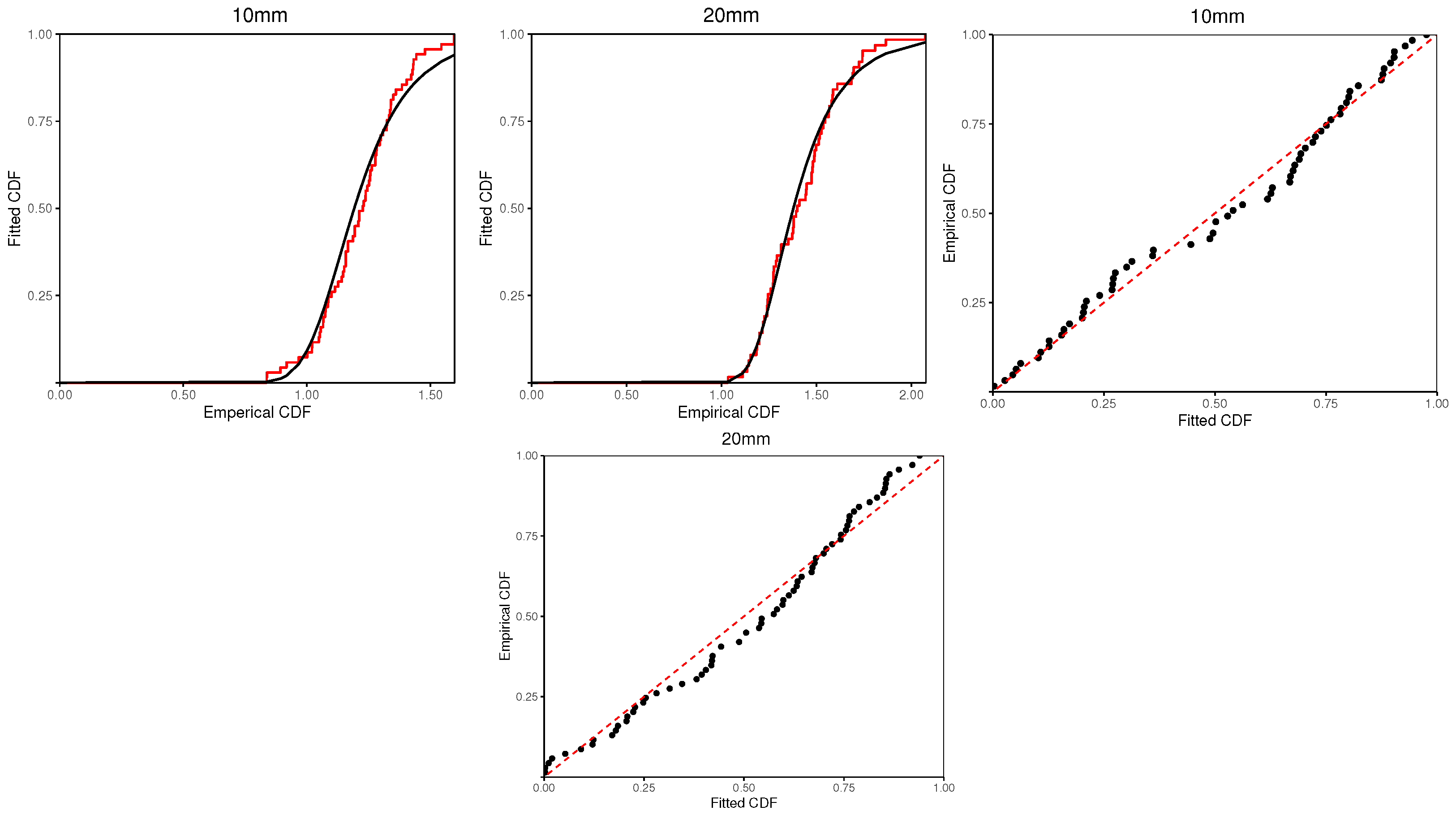
Before proceeding, assessment of goodness-of-fit is conducted to check if the BIII model can be used as a proper model to fit these data. The Kolmogorov–Smirnov (KS) distances and the associated p-values (with brackets) are obtained as 0.0984 (0.5137) and 0.1040 (0.4824), respectively. The Anderson–Darling (AD) test statistic and the associated p-values (with brackets) are 1.0411 (0.3612) and 1.3095 (0.3286), respectively. Therefore, these results indicate that the BIII distribution is a suitable model for these real-world datasets under different cases. In addition, Figure 2 illustrates a comparison between the empirical cumulative distribution function and the fitted BIII distribution, complemented by Probability–Probability (P-P) plots. These plots also show that the BIII distribution can be used as a suitable model to fit the data visually.
In our example, the carbon fiber strength data for 10 mm and 20 mm are treated as two-cycle data to show the application of the proposed methods, i.e., the data for 10 mm are assumed from BIII ( c 1 , θ 1 ) and the data for 20 mm from BIII ( c 2 , θ 2 ) , respectively. Further, the null hypothesis is H 0 : c 1 = c 2 = c , and the alternative hypothesis is H 1 : c 1 c 2 . Based on direct calculation, the value of the LRT statistic and the associated p-value are 0.7867 and 0.8039. Therefore, there is insufficient evidence to reject the null hypothesis H 0 , and it is assumed that these two datasets from 10 mm and 20 mm follow the BIII populations with parameters ( c , θ 1 ) and ( c , θ 2 ) in consequence.
Following the sampling scenario of MaxRSSU, two sets of the MaxRSSU data of sizes n 1 = 10 and n 2 = 11 are generated from the original carbon fibers data for 10 mm and 20 mm, respectively. The detailed, procedures are shown as follows:
MaxRSSU sampling MaxRSSU 1 : 1.1523 1.1523 2 : 1.3923 1.6840 1.6840 3 : 1.3760 1.4880 1.5107 1.5107 4 : 1.4463 1.4907 1.6903 1.7237 1.7237 5 : 1.2713 1.2747 1.3133 1.3790 1.5873 1.5873 6 : 1.1343 1.1427 1.1990 1.2440 1.6953 1.7423 1.7423 7 : 1.1987 1.2417 1.2583 1.2720 1.4483 1.4980 2.0733 2.0733 8 : 1.2407 1.3723 1.3987 1.4100 1.4810 1.5257 1.5450 1.5790 1.5790 9 : 1.0337 1.1107 1.2150 1.2180 1.2917 1.3127 1.4743 1.6093 1.8083 1.8083 10 : 1.1833 1.2393 1.3520 1.4733 1.4783 1.5153 1.5360 1.5670 1.5847 1.7413 1.7413
and
MaxRSSU sampling MaxRSSU 1 : 1.0203 1.0203 2 : 1.4223 1.5950 1.5950 3 : 1.0657 1.1567 1.5443 1.5443 4 : 1.1940 1.2300 1.2947 1.3600 1.3600 5 : 0.9173 1.0667 1.2807 1.3393 1.4300 1.4300 6 : 0.8373 1.0850 1.1133 1.1413 1.2553 1.2990 1.2990 7 : 1.0527 1.0737 1.1263 1.1467 1.2117 1.3847 1.5950 1.5950 8 : 1.0993 1.1573 1.1940 1.2370 1.2380 1.2763 1.3087 1.3363 1.3363 9 : 1.0877 1.1510 1.2620 1.3243 1.3333 1.3493 1.4280 1.4427 1.4777 1.4777 10 : 1.0480 1.0553 1.0757 1.1580 1.1670 1.1670 1.2087 1.2260 1.2777 1.4040 1.4040 11 : 0.8930 0.9667 1.0010 1.0217 1.2113 1.2450 1.2567 1.2827 1.3233 1.3403 1.4320 1.4320
Therefore, two sets of MaxRSSU data are obtained as follows:
First - cycle MaxRSSU data : 1.1523 , 1.6840 , 1.5107 , 1.7237 , 1.5873 , 1.7423 ,     2.0733 , 1.5790 , 1.8083 , 1.7413 Sec ond - cycle MaxRSSU data : 1.0203 , 1.5950 , 1.5443 , 1.3600 , 1.4300 , 1.2990 ,     1.5950 , 1.3363 , 1.4777 , 1.4040 , 1.4320
Based on the above MaxRSSU data with two-cycle, classical likelihood and Bayes estimates are computed by using the proposed methods when accounting for the DBDC effect. The associated results are presented in Table 6, where the estimated standard errors (ESE) for the point estimates and the interval lengths are provided in square brackets, and the interval estimates are obtained for a 95 % significance level. In addition, for the Bayes estimates, the results are obtained based on 10,000 reputations, and the first 5000 samples are discarded to ensure convergence.
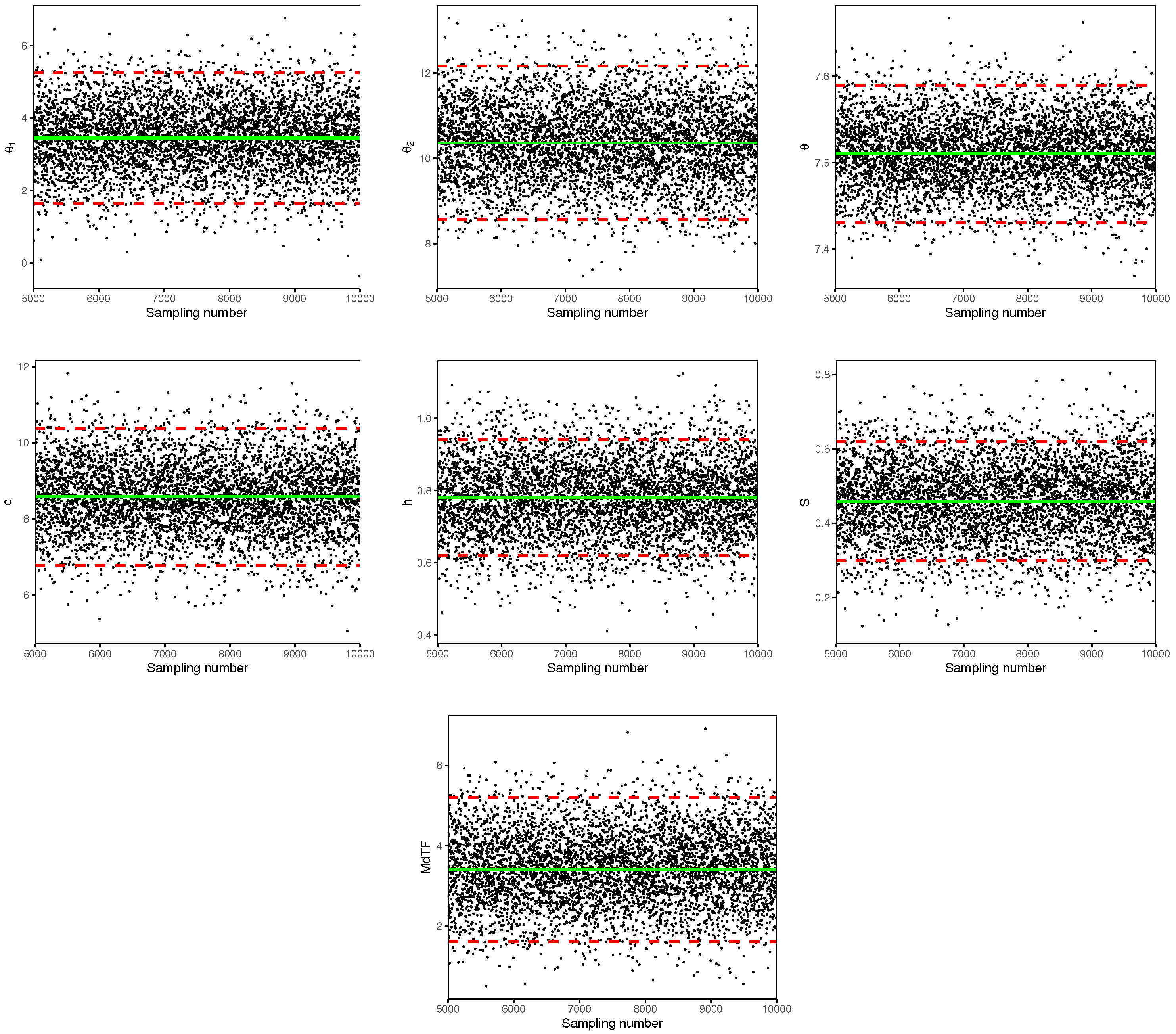
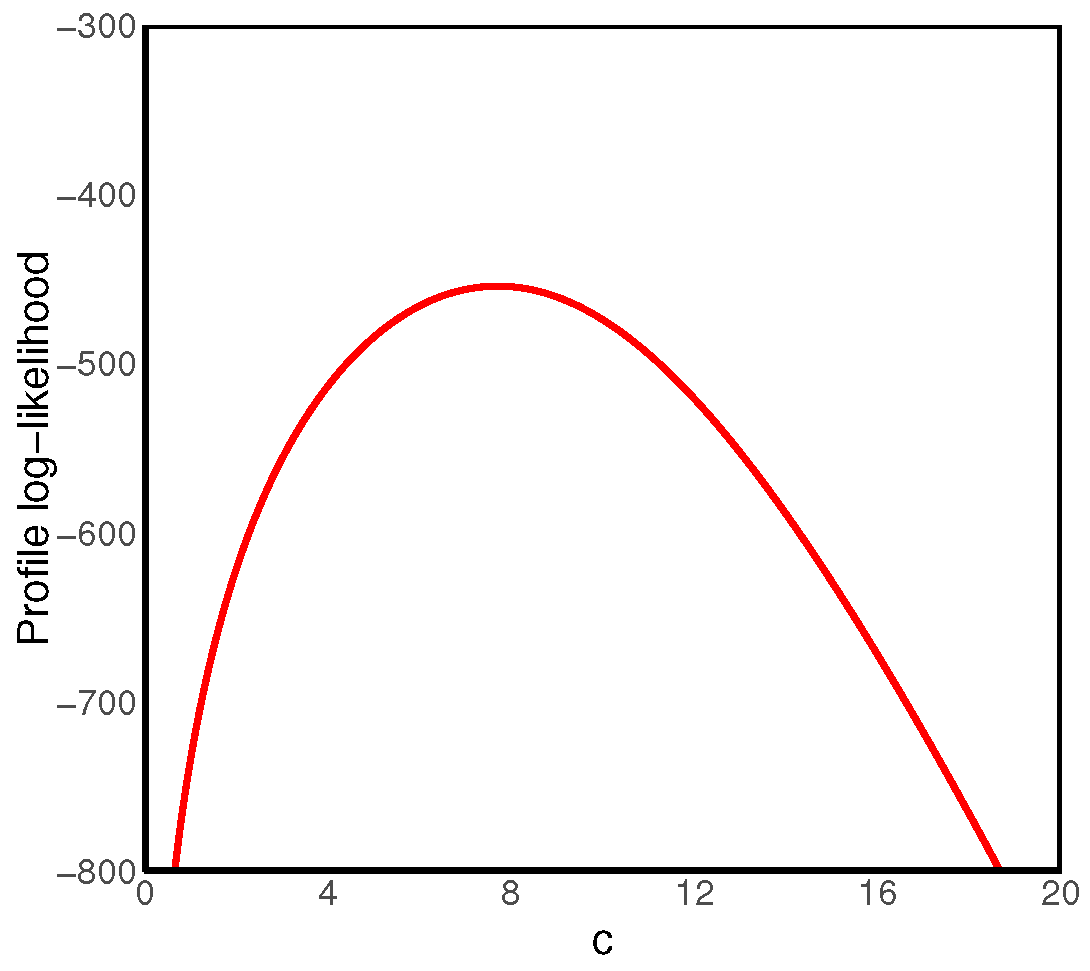
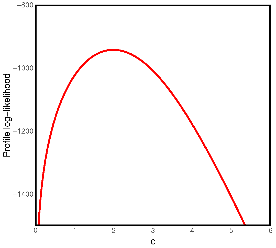
Based on Table 6, it can be observed that, for different parameters and reliability indices, both the MLEs and the Bayes estimates perform satisfactorily. Moreover, in terms of the ESE, the Bayes estimates generally outperform the corresponding MLEs. Similarly, the HPD credible intervals tend to have shorter lengths compared to the ACIs, indicating the superior performance of the hierarchical Bayesian method. In addition, the partial overlapping among different interval estimates for the same parameters and reliability indices under classical and Bayesian approaches suggests that the cycle effects may not be ignorable. Furthermore, to investigate the performance of the Bayesian sampling method, Figure 3 provides trace plots for parameters c , θ 1 , θ 2 , and reliability indices S ( 0.8 ) , h ( 0.8 ) and MdTF, where a solid line denotes the associated Bayes estimate, and the dashed lines give the associated interval bounds. It is noted that there is good mixing performance of the proposed Bayes sampling approach. In addition, the plots of the profile log-likelihood function of the parameter c are also presented in Figure 4. It is also observed that the profile function is a unimodal function showing the existence and uniqueness of the MLE c ^ that is consistent with Theorem 2.
Example two (bank waiting times datasets). As another example, the waiting times (in minutes) before customer service in two different banks are discussed. The original data were provided in Ghitany et al. [36]. The detailed waiting time data are shown in Table 7.
Before proceeding further, the goodness-of-fit is assessed to determine if the BIII distribution can serve as a reasonable model. Based on the complete data shown in Table 7, the KS distances and the p-values (with brackets) for the original data from Bank A and Bank B are 0.1062 (0.3124) and 0.1337 (0.2946), respectively. The AD statistic and the associated p-values (with brackets) are 2.0682 (0.2841) and 1.9037 (0.2593), respectively. These results suggest that the BIII model can be used as an appropriate model for the bank waiting times data. Furthermore, Figure 5 also shows the empirical cumulative distribution function, the fitted BIII distribution, and the P-P plots. These plots also show that the BIII distribution can be used as a suitable model to fit the data visually.
In this example, the waiting times data from Bank A and Bank B are treated as two-cycle data to demonstrate the application of the proposed methods. Specifically, the data from Bank A are assumed to follow a BIII ( c 1 , θ 1 ) distribution, while those from Bank B are assumed to follow a BIII ( c 2 , θ 2 ) distribution. Similarly to Example one, the LRT statistic and the p-value are calculated as 0.5867 and 0.2832. Therefore, the null hypothesis c 1 = c 2 = c holds and we use BIII ( c , θ 1 ) and BIII ( c , θ 2 ) to fit the real-life bank A and bank B data, respectively.
Following the MaxRSSU scenario, a set of MaxRSSU data with size n 1 = 5 from Bank A and size n 2 = 5 from Bank B are obtained as follows:
First - cycle MaxRSSU data : 5.0 , 13.7 , 11.1 , 27.0 , 19.0 Sec ond - cycle MaxRSSU data : 5.3 , 12.1 , 8.0 , 14.5 , 3.5
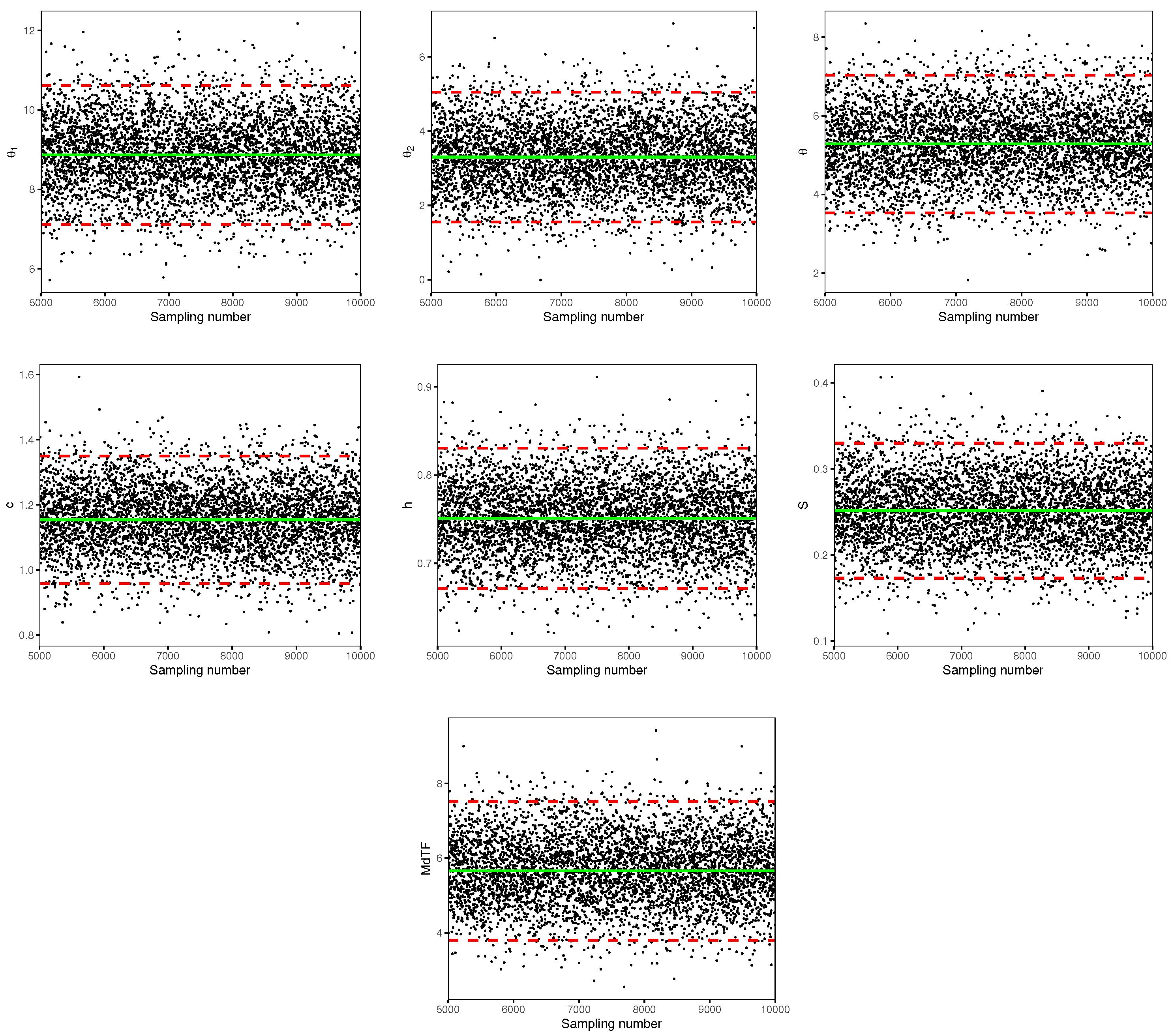
Consequently, classical likelihood and Bayes estimates of the parameters and reliability indices are conducted for the bank MaxRSSU data with DBDC effect. The results are summarized in Table 8 with a 95 % significance level for the confidence level. Based on the results tabulated in Table 8, it can also be observed that the hierarchical Bayesian method outperforms the traditional likelihood approach for both point and interval estimates in general. For completeness, the trace plots and the curve of the profile log-likelihood function of c are also shown in Figure 6 and Figure 7 for illustration.

7. Conclusions

This paper investigates statistical inference for multiple-cycle MaxRSSU data using the BIII distribution, focusing on scenarios with non-ignorable cycle effects. MLE is employed, and the existence and uniqueness of the model parameters are established. A hierarchical Bayesian approach is also proposed, with MH sampling used for posterior computation. Simulation and real-data studies show that both methods perform well, with the Bayesian approach generally offering better estimation accuracy and flexibility. Although the study focuses on the BIII distribution, the methods can be extended to other models, such as the Kies or exponentiated Rayleigh models with suitable adjustments. Future work will focus on optimizing the design of the MaxRSSU scheme under time and cost constraints. This includes optimizing the key parameters, such as sample allocation and number of cycles, to improve its practical value and efficiency in reliability testing. Additionally, extending the statistical inference methods of the multiple-cycle model to other data types, such as record values and standard RSS, to handle more complex data collection scenarios, is also a promising direction for further research.

Author Contributions

Conceptualization, L.W. and Z.C.; methodology, L.W.; software, Z.C. and Y.M.T.; writing—original draft preparation, Z.C. and L.W.; writing—review and editing, L.W. and Y.L. All authors have read and agreed to the published version of the manuscript.

Funding

The work of Liang Wang was supported by the Yunnan Fundamental Research Projects (No. 202401AT070116), the Yunnan Key Laboratory of Modern Analytical Mathematics and Applications (No. 202302AN360007), and the Cross-integration Innovation team of Modern Applied Mathematics and Life Sciences in Yunnan Province, China (202405AS350003). The work of Zirui Chu was supported by the Yunnan Provincial Department of the Education Science Research Fund Project (No. 2025Y0328).

Data Availability Statement

No new data were created or analyzed in this study. Data sharing is not applicable to this article.

Acknowledgments

The authors would like to thank the Editor and reviewers for their valuable comments and suggestions which improved the paper significantly.

Conflicts of Interest

The authors declare no conflicts of interest.

References

  1. McIntyre, G.A. A method for unbiased selective sampling using ranked sets. Aust. J. Agric. Res. 1952, 3, 385–390. [Google Scholar] [CrossRef]
  2. Bouza, C.N. Ranked set sampling and randomized response procedures for estimating the mean of a sensitive quantitative character. Metrika 2009, 70, 267–277. [Google Scholar] [CrossRef]
  3. He, X.; Chen, W.; Qian, W. Maximum likelihood estimators of the parameters of the log-logistic distribution. Stat. Pap. 2020, 61, 1875–1892. [Google Scholar] [CrossRef]
  4. Taconeli, C.A.; Bonat, W.H. On the performance of estimation methods under ranked set sampling. Comput. Stat. 2020, 35, 1805–1826. [Google Scholar] [CrossRef]
  5. Nawaz, T.; Han, D. Monitoring the process location by using new ranked set sampling-based memory control charts. Qual. Technol. Quant. Manag. 2019, 17, 255–284. [Google Scholar] [CrossRef]
  6. Qian, W.; Chen, W.; He, X. Parameter estimation for the Pareto distribution based on ranked set sampling. Stat. Pap. 2021, 62, 395–417. [Google Scholar] [CrossRef]
  7. Dumbgen, L.; Zamanzade, E. Inference on a distribution function from ranked set samples. Ann. Inst. Stat. Math. 2020, 72, 157–185. [Google Scholar] [CrossRef]
  8. Samawi, H.M.; Ahmed, M.S.; Abu-Dayyeh, W. Estimating the population mean using extreme ranked set sampling. Biom. J. 1996, 38, 577–586. [Google Scholar] [CrossRef]
  9. Hussain, S.A.; Ahmad, I.; Saghir, A.; Aslam, M.; Almanjahie, I.M. Mean ranked acceptance sampling plan under exponential distribution. Ain Shams Eng. J. 2021, 12, 4125–4131. [Google Scholar] [CrossRef]
  10. Muttlak, H.A. Investigating the use of quartile ranked set samples for estimating the population mean. Appl. Math. Comput. 2003, 146, 437–443. [Google Scholar] [CrossRef]
  11. Hossain, S.S.; Muttlak, H.A. Paired ranked set sampling: A more efficient procedure. Environmetrics 1999, 10, 195–212. [Google Scholar] [CrossRef]
  12. Al-Saleh, M.F.; Al-Omari, A.I. Multistage ranked set sampling. J. Stat. Plan. Inference 2002, 102, 273–286. [Google Scholar] [CrossRef]
  13. Mahdizadeh, M.; Zamanzade, E. Stratified pair ranked set sampling. Commun. -Stat.-Theory Methods 2018, 47, 5904–5915. [Google Scholar] [CrossRef]
  14. Bhoj, D.S. Ranked set sampling with unequal samples. Biometrics 2001, 57, 957–962. [Google Scholar] [CrossRef]
  15. Eskandarzadeh, M.; Di Crescenzo, A.; Tahmasebi, S. Measures of information for maximum ranked set sampling with unequal samples. Commun. -Stat.-Theory Methods 2018, 47, 4692–4709. [Google Scholar] [CrossRef]
  16. Qiu, G.; Eftekharian, A. Extropy information of maximum and minimum ranked set sampling with unequal samples. Commun. Stat.-Theory Methods 2020, 50, 1–17. [Google Scholar] [CrossRef]
  17. Basikhasteh, M.; Lak, F.; Afshari, M. Bayesian estimation of stress-strength reliability for two parameter bathtub-shaped lifetime distribution based on maximum ranked set sampling with unequal samples. J. Stat. Comput. Simul. 2020, 90, 1–16. [Google Scholar] [CrossRef]
  18. Wolfe, D.A. Ranked set sampling: Its relevance and impact on statistical inference. Int. Sch. Res. Not. 2012, 2012, 568385. [Google Scholar] [CrossRef]
  19. Wang, X.; Lim, J.; Stokes, L. Using ranked set sampling with cluster randomized designs for improved inference on treatment effects. J. Am. Stat. Assoc. 2016, 111, 1576–1590. [Google Scholar] [CrossRef]
  20. Akdeniz, S.; Yildiz, T.O. The effects of ranking error models on mean estimators based on ranked set sampling. Revstat-Stat. J. 2023, 21, 347–366. [Google Scholar]
  21. Ahmadi, M.; Doostparast, M.; Ahmadi, J. Block censoring scheme with two-parameter exponential distribution. J. Stat. Comput. Simul. 2018, 88, 1229–1251. [Google Scholar] [CrossRef]
  22. Zhu, T. Reliability estimation for two-parameter Weibull distribution under block censoring. Reliab. Eng. Syst. Saf. 2020, 203, 107071. [Google Scholar] [CrossRef]
  23. Kumari, R.; Tripathi, Y.M.; Gangopadhyay, A.K.; Lodhi, C. Reliability inference for Gompertz distribution using pivotal method under block progressive Type-II censored data. Res. Sq. 2024; published online. [Google Scholar] [CrossRef]
  24. Wang, L.; Wu, S.J.; Lin, H.; Tripathi, Y.M. Inference for block progressive censored competing risks data from an inverted exponentiated exponential model. Qual. Reliab. Eng. Int. 2023, 39, 2736–2764. [Google Scholar] [CrossRef]
  25. Kim, C.; Kim, W. Estimation of the Parameters of Burr Type III Distribution Based on Dual Generalized Order Statistics. Sci. World J. 2014, 2014, 512039. [Google Scholar] [CrossRef] [PubMed]
  26. Cordeiro, G.; Gomes, A.; da-Silva, C.; Ortega, E.M. A useful extension of the Burr III distribution. J. Stat. Distrib. Appl. 2017, 4, 24. [Google Scholar] [CrossRef]
  27. Domma, F. Some properties of the bivariate Burr type III distribution. Statistics 2010, 44, 203–215. [Google Scholar] [CrossRef]
  28. Singh, S.; Belaghi, R.A.; Asl, M.N. Estimation and prediction using classical and Bayesian approaches for Burr III model under progressive Type-I hybrid censoring. Int. J. Syst. Assur. Eng. Manag. 2019, 10, 746–764. [Google Scholar] [CrossRef]
  29. Omea, A.; Mehmet, N.C.; Abdullah, Y. Statistical inference for the Burr Type-III distribution under Type-II censored data. Appl. Math. Model. 2017, 66, 297–310. [Google Scholar]
  30. Feroze, N.; Aslam, M.; Sindhu, T.N. On maximum likelihood estimation for left censored Burr Type-III distribution. Pak. J. Stat. Oper. Res. 2015, 11, 497–512. [Google Scholar] [CrossRef]
  31. Barndorff-Nielsen, O.E.; Cox, D.R. Inference and Asymptotics; Chapman and Hall: New York, NY, USA, 1994. [Google Scholar]
  32. Wingo, D.R. Maximum likelihood methods for fitting the burr Type XII distribution to multiply (progressively) censored life test data. Metrika 1993, 40, 203–210. [Google Scholar] [CrossRef]
  33. Singh, D.P.; Jha, M.K.; Tripathi, Y.M.; Wang, L. Reliability estimation in a multicomponent stress-strength model for unit Burr III distribution under progressive censoring. Qual. Technol. Quant. Manag. 2022, 19, 605–632. [Google Scholar] [CrossRef]
  34. Badar, M.G.; Priest, A.M. Statistical aspects of fiber and bundle strength in hybrid composites. Int. Consort. Chin. Math. 1982, 6, 1129–1136. [Google Scholar]
  35. Mead, M.E.; Afify, A.Z.; Hamedani, G.G.; Ghosh, I. The Beta exponential Frechet distribution with applications: Properties and applications. Aust. New Zealand J. Stat. 2017, 46, 41–63. [Google Scholar]
  36. Ghitany, M.E.; Atieh, B.; Nadarajah, S. Lindley distribution and its application. Math. Comput. Simul. 2008, 78, 493–506. [Google Scholar] [CrossRef]
Figure 1. Plots of PDF and HRF of the BIII with different parameters.
Axioms 14 00619 g001
Figure 2. Empirical distribution and fitted BIII distribution, P-P plot for the carbon fibers data.
Axioms 14 00619 g002
Figure 3. Trace plots for the parameters and reliability indices for the carbon fibers data.
Axioms 14 00619 g003
Figure 4. Profile log-likelihood function of c for the carbon fibers data.
Axioms 14 00619 g004
Figure 5. Empirical distribution and fitted BIII distribution, P-P of bank waiting times data.
Axioms 14 00619 g005
Figure 6. Trace plots for the parameters and reliability indices for bank waiting times data.
Axioms 14 00619 g006
Figure 7. Profile log-likelihood of parameter c for bank waiting times data.
Axioms 14 00619 g007
Table 1. MSEs, ABs, and ALs for parameters θ = 0.8 , c = 0.9 with k = 2 .
n 1 n 2 par.MLEACIBayesHPD
MSEABLowerUpperLengthMSEABLowerUpperLength
55 θ 1 0.85900.4497−0.09561.97412.06970.27030.37550.28151.17061.4241
θ 2 0.81750.4567−0.07722.02512.10230.28630.29140.29701.67131.3743
θ 0.16920.27850.23621.16340.92720.24770.25840.39921.25710.8579
c0.74650.6297−0.19892.65512.85400.41720.52970.92452.18901.2645
MdTF0.20510.21570.17311.20001.02690.25560.15600.33421.25780.9236
S ( t ) 0.03170.02170.38880.92940.54060.01230.01830.47680.88960.4128
h ( t ) 0.15720.33270.44971.63101.18130.04560.18720.54221.32050.7782
7 θ 1 0.78240.42180.02562.24532.21970.18920.28970.41011.76381.3536
θ 2 0.80270.43000.05792.12802.07010.11970.24080.45921.70271.2435
θ 0.15030.29080.37041.41361.04310.12980.24810.56831.53260.9642
c0.36120.4988−0.08381.97472.05850.16580.39740.82621.79810.9718
MdTF0.19250.27960.15921.50031.34110.15000.21050.46121.54981.0886
S ( t ) 0.02510.02510.46140.91990.45840.02270.02270.54780.91020.3625
h ( t ) 0.14770.22320.32051.41551.09500.02570.11790.43521.06700.6318
88 θ 1 0.38150.37630.30621.82151.51530.13240.25820.50011.73851.2384
θ 2 0.49900.39500.32691.87821.55130.15880.28020.51971.79271.2730
θ 0.16010.28600.54921.37090.82170.15160.29120.63441.57510.9407
c0.19900.3770−0.07411.87431.94840.13310.35550.86381.67190.8081
MdTF0.19960.31210.34041.47131.13080.14610.35890.52871.57741.0487
S ( t ) 0.02520.02520.51790.89820.38030.02140.02640.57600.91300.3370
h ( t ) 0.05230.17640.27751.32061.04300.02700.11860.42380.98520.5615
10 θ 1 0.29780.34180.36601.66421.29810.10750.23310.47791.69431.2164
θ 2 0.38670.35760.29471.84631.55160.09060.21440.51181.67961.1678
θ 0.15310.28150.57461.31660.74200.10770.24970.61891.50700.8881
c0.17400.3634−0.02371.94571.96940.12340.34330.87381.63290.7591
MdTF0.18960.31250.38861.40461.01600.14990.31900.51431.51380.9995
S ( t ) 0.02470.02470.51650.89110.37460.02240.02240.56680.90410.3373
h ( t ) 0.05180.17980.29011.32241.03230.01860.09820.45240.99350.5411
Table 2. MSEs, ABs, and ALs for parameters θ = 0.7 , c = 1 with k = 2 .
n 1 n 2 par.MLEACIBayesHPD
MSEABLowerUpperLengthMSEABLowerUpperLength
46 θ 1 0.95700.4908−0.02902.05812.08710.21980.31980.35921.71981.3606
θ 2 0.81270.5251−0.01372.30662.32030.14240.26140.40421.68531.2811
θ 0.34680.38600.27731.37681.09950.16190.28700.51301.48250.9695
c0.59310.6203−0.06702.29582.36270.19670.42690.86332.03431.1710
MdTF0.26320.37550.17191.39601.22410.21610.36450.42841.48821.0598
S ( t ) 0.03150.03150.43750.94630.50880.03130.03130.53170.91570.3839
h ( t ) 0.09570.23990.36711.50741.14020.04350.15300.43891.15920.7203
8 θ 1 0.90690.4241−0.08451.87101.95550.21980.32170.37041.71751.3471
θ 2 0.72160.38350.08241.92771.84530.07880.19550.41191.50901.0971
θ 0.22740.26280.28811.37261.08440.12340.25620.51621.42430.9081
c0.44580.53880.06412.09962.03550.19530.42950.91401.98121.0672
MdTF0.14500.26780.15881.40861.24970.16370.33190.44061.40080.9602
S ( t ) 0.03080.03080.46880.91190.44320.02930.02930.53580.91090.3751
h ( t ) 0.08310.22040.37251.45571.08320.03320.13020.46551.14810.6825
77 θ 1 0.64780.40740.15072.17342.02270.16480.29640.49391.82321.3293
θ 2 0.36610.32890.19271.69641.50370.05670.18470.41541.58681.1713
θ 0.19550.26130.44461.34020.89550.16290.31860.57431.49910.9249
c0.36240.4173−0.29291.64781.94070.12580.34390.89481.82500.9303
MdTF0.13630.24720.28241.40681.12430.15380.39480.48421.48320.9990
S ( t ) 0.03190.03190.47830.93390.45550.03090.03290.55770.91240.3547
h ( t ) 0.06190.18420.31891.38291.06390.03120.15150.44211.06270.6206
9 θ 1 0.59840.36480.18891.98221.79340.08520.20710.39021.58691.1967
θ 2 0.17480.22550.13961.38651.24700.03310.12450.33821.25350.9153
θ 0.11150.20890.37451.13800.76360.04090.13870.46001.22320.7631
c0.33680.5781−0.05681.77001.82680.11780.21921.03882.03420.9954
MdTF0.09400.22320.31411.15540.84130.06850.21510.40361.19690.7933
S ( t ) 0.02580.02580.46570.89490.42920.02020.02020.51310.88920.3761
h ( t ) 0.06740.21200.48391.45730.97340.01530.09460.56381.12400.5602
Table 3. MSEs, ABs, and ALs for parameters θ = 0.5 , c = 1.5 with k = 3 .
n 1 n 2 n 3 par.MLEACIBayesHPD
MSEABLowerUpperLengthMSEABLowerUpperLength
455 θ 1 0.32430.4291−0.03211.68961.72170.04190.12850.17261.24891.0763
θ 2 0.26580.40230.03281.59401.56120.02780.10020.20021.18170.9815
θ 3 0.37880.26310.00821.26891.26070.02330.09100.16941.04970.8804
θ 0.03460.13590.19410.80540.61130.02970.11270.31950.92760.6081
c0.87910.92201.48992.75061.26070.80550.86701.03671.96800.9313
MdTF0.15450.37380.25770.87360.61600.12860.33520.29380.96190.6681
S ( t ) 0.14260.10430.39650.83640.43990.04000.04000.43690.83450.3976
h ( t ) 0.16320.34730.78301.75850.97550.13390.09580.74171.49240.7507
56 θ 1 0.18680.2345−0.00421.05751.06170.00950.07080.09330.87610.7828
θ 2 0.28700.23360.02661.07491.04830.03430.13580.11820.86700.7488
θ 3 0.14210.21070.06111.00600.94480.00290.03770.13490.83020.6953
θ 0.02960.14430.15890.62940.47050.00610.05440.22350.68960.4662
c0.75880.76541.24822.19300.94480.39970.62351.49252.38510.8926
MdTF0.07200.23280.27080.77950.50870.05790.22910.27630.80670.5304
S ( t ) 0.03660.03660.39120.81450.42330.01790.01790.41260.81730.4046
h ( t ) 0.27150.47230.95851.87560.91710.03920.18960.90351.73590.8323
668 θ 1 0.15800.24190.08421.18611.10190.00770.06300.17490.97610.8012
θ 2 0.13340.21080.06611.09661.03050.00520.05360.16290.92860.7657
θ 3 0.11170.21050.06611.20731.14120.00330.04320.21130.96580.7545
θ 0.02650.10690.24510.72770.48270.00600.06640.30540.78000.4746
c0.63410.72121.04142.18261.14120.64920.71441.30232.82781.5255
MdTF0.09150.22520.29290.82510.53230.06660.25300.32450.85790.5333
S ( t ) 0.03850.03450.41300.81870.40560.03040.03040.45270.82660.3738
h ( t ) 0.14900.34580.88431.69100.80670.03700.08270.85141.54690.6955
78 θ 1 0.05800.14500.08820.90870.82060.00610.05590.16490.88890.7239
θ 2 0.70770.8864−0.06201.56111.62310.00520.05070.35931.56061.2013
θ 3 0.03880.13710.13610.90080.76470.00440.04770.19560.85040.6548
θ 0.01830.09480.24880.72260.47380.00370.04270.31920.79570.4765
c0.95510.90900.91492.19141.27650.63440.63880.97412.11191.1379
MdTF0.06820.21880.22360.79780.57420.09420.30180.22170.82440.6027
S ( t ) 0.02600.02600.37380.77750.40370.03880.03880.39110.75980.3687
h ( t ) 0.12590.32130.89971.64070.74100.06080.06390.86501.44260.5777
Table 4. MSEs, ABs, and ALs for parameters θ = 0.6 , c = 0.5 with k = 3 .
n 1 n 2 n 3 par.MLEACIBayesHPD
MSEABLowerUpperLengthMSEABLowerUpperLength
555 θ 1 0.82870.25740.00440.99710.99270.04170.19660.10630.80540.6991
θ 2 0.94530.32560.02331.18971.16640.02340.14130.12060.90440.7839
θ 3 0.24360.27390.01331.05181.03840.01710.11960.11190.84770.7358
θ 0.07380.24750.13960.58940.44970.02860.16370.21790.67970.4617
c0.70060.63371.31782.35631.03840.53450.43210.94911.89520.9461
MdTF0.04940.17080.10340.62560.52220.04470.20570.13290.63470.5018
S ( t ) 0.01450.01450.28450.66010.37560.00660.00660.32030.70350.3831
h ( t ) 0.76050.84340.93041.95271.02230.49120.69590.92551.67590.7504
67 θ 1 0.77290.23840.05061.33061.28010.03110.16240.13980.98100.8412
θ 2 0.10550.22670.06390.97040.90650.01440.11060.13650.82760.6912
θ 3 0.08020.20120.07090.90910.83820.01320.10790.14570.78180.6361
θ 0.06480.21910.18810.61490.42680.02200.14410.24660.68650.4399
c0.64310.52241.30492.14310.83820.50520.40150.90031.16290.7289
MdTF0.06240.18830.13370.69980.56610.04410.20490.12940.65450.5251
S ( t ) 0.01470.01870.32830.69390.36570.00650.00650.31170.67050.3588
h ( t ) 0.64230.77750.93441.81440.88000.42010.64490.91331.58510.6718
778 θ 1 0.09670.22270.11660.92340.80680.01760.12520.15530.82700.6718
θ 2 0.06360.25550.09960.85980.76020.01350.10950.14190.76520.6233
θ 3 0.11530.16590.12581.03960.91370.01970.13260.18060.86470.6841
θ 0.05260.17470.22240.61130.38880.02170.14390.26290.66560.4027
c0.46070.41691.21242.12610.91370.42840.31261.04061.76320.7226
MdTF0.05960.19670.18150.70610.52460.05520.18150.15620.65070.4945
S ( t ) 0.01410.01520.35560.70430.34860.00960.00960.33100.66920.3382
h ( t ) 0.58840.74880.96511.72730.76220.45840.67510.97911.57690.5978
99 θ 1 0.08100.21280.10631.01620.90990.01810.12510.17400.90030.7263
θ 2 0.17070.18300.06301.24631.18330.02200.13970.21750.93240.7149
θ 3 0.04530.23850.13600.80440.66840.01480.11630.17580.74800.5722
θ 0.03820.20230.29380.69390.40000.01390.11400.24710.64230.3952
c0.31580.38050.91681.88300.96610.28760.23401.21241.88080.6684
MdTF0.06300.20530.15920.69730.53810.04800.15460.15260.67580.5231
S ( t ) 0.01420.01320.33240.68250.35010.00720.00720.35060.68160.3311
h ( t ) 0.48870.68390.91631.64950.73330.34360.58490.92891.44670.5178
Table 5. Testing data of the single carbon fibers with different diameters.
LengthStrength Data
10 mm1.15231.39231.68401.48801.51071.37601.49071.44631.72371.6903
1.58731.37901.27471.27131.31331.74231.14271.19901.24401.1343
1.69531.24171.19871.49801.25831.44832.07331.27201.48101.3987
1.54501.52571.24071.41001.37231.57901.47431.29171.21501.0337
1.11071.21801.60931.80831.31271.56701.58471.47831.35201.1833
1.53601.23931.74131.51531.47331.44171.86501.18701.28631.2727
1.22471.37901.5643
20 mm1.02031.59501.42231.54431.15671.06571.23001.19401.29471.3600
0.91731.43001.28071.06671.33931.25530.83731.29901.11331.0850
1.14131.14671.38471.59501.05271.21171.12631.07371.19401.0993
1.15731.30871.23801.23701.33631.27631.08771.47771.34931.4280
1.26201.15101.32431.33331.44271.05531.22601.15801.16701.1670
1.27771.04801.40401.07571.20871.43201.00101.32331.21131.2567
1.28270.89301.02170.96671.24501.34031.25130.83801.1863
Table 6. Point and interval estimates of carbon fibers data.
par.MLEACIBayesHPD
θ 1 3.5070 [0.2146](1.7423, 5.3396) [3.5973]3.2354 [0.1052](1.6131, 5.2781) [3.6650]
θ 2 10.7983 [0.7462](8.5713, 13.1678) [4.5965]10.6924 [0.6959](8.5832, 12.0945) [3.5113]
θ 7.2119 [0.0077](7.0770, 7.6569) [0.5799]7.5148 [0.0054](7.4326, 7.5925) [0.1599]
c8.9746 [1.0591](6.7696, 10.5796) [4.8100]8.7810 [0.9446](6.9102, 10.5749) [3.6647]
MdTF3.7669 [0.6997](1.5735, 4.9602) [3.3867]3.3431 [0.2457](1.7343, 5.1638) [3.4295]
S ( 1.1 ) 0.4766 [0.5174](0.3079, 0.6452) [0.3373]0.4608 [0.2661](0.3146, 0.6233) [0.3087]
h ( 1.1 ) 0.8717 [0.7416](0.5045, 0.9839) [0.4794]0.7886 [0.4902](0.6170, 0.9424) [0.3254]
Table 7. Data for the waiting times (in minutes) before customer service at the bank.
BankWaiting Time Data
A5.013.78.23.311.16.98.07.127.04.619.011.28.9
2.612.44.71.921.918.26.113.621.313.13.55.317.3
15.46.74.44.79.68.613.018.911.96.219.95.74.9
1.82.13.13.24.15.511.010.911.04.313.312.57.4
17.338.53.64.91.933.111.54.321.46.27.74.010.7
1.58.99.76.323.04.28.64.213.99.820.618.11.3
15.47.19.57.64.47.114.111.218.431.67.12.78.8
2.98.86.20.84.812.95.78.60.8
B5.32.512.12.30.38.011.08.06.814.53.52.92.7
0.91.24.21.94.56.31.810.910.78.53.96.616.0
2.72.316.52.02.37.57.38.528.03.43.112.83.4
1.10.29.57.75.65.64.73.10.18.72.26.23.2
12.312.92.613.20.713.74.07.7
Table 8. Point and interval estimates of bank waiting times data.
par.MLEACIBayesHPD
θ 1 9.0293 [ 0.9319](7.1293, 11.0247) [3.8954]8.9245 [0.7472](7.0929, 10.6830) [3.5901]
θ 2 3.2869 [0.7048](1.4962, 5.0682) [3.5720]3.2936 [0.6947](1.5815, 5.0681) [3.4866]
θ 5.1803 [0.7259](4.0137, 9.0168) [5.0031]5.2853 [0.5835](3.5862, 7.0938) [3.5076]
c1.2963 [0.2865](0.9028, 1.3985) [0.4957]1.1727 [0.0928](0.9625, 1.3730) [0.4105]
MdTF5.8243 [0.7739](3.7653, 7.9023) [4.1370]5.6034 [0.6926](3.8926, 7.4947) [3.6021]
S ( 0.8 ) 0.3051 [0.2936](0.1961, 0.4629) [0.2668]0.2592 [0.0962](0.1792, 0.3381) [0.1589]
h ( 0.8 ) 0.7240 [0.5139](0.6492, 0.8720) [0.2228]0.7528 [0.3826](0.6528, 0.8472) [0.1944]
Disclaimer/Publisher’s Note: The statements, opinions and data contained in all publications are solely those of the individual author(s) and contributor(s) and not of MDPI and/or the editor(s). MDPI and/or the editor(s) disclaim responsibility for any injury to people or property resulting from any ideas, methods, instructions or products referred to in the content.