Failure Cause Analysis Under Progressive Type-II Censoring Using Generalized Linear Exponential Competing Risks Model with Medical and Industrial Applications ^†

Abstract

This study focuses on analyzing progressive Type-II right censoring competing risks datasets. The latent causes of failures are assumed to follow independent generalized linear exponential distributions. The maximum likelihood and maximum product of spacing methods are employed to estimate the unknown parameters and survival indices. Furthermore, approximate confidence intervals are derived using the asymptotic normality of the maximum likelihood and the maximum product of spacing estimators. Additionally, bootstrap methods are employed to construct confidence intervals. A comprehensive simulation study is carried out to evaluate the effectiveness of these estimation approaches. Finally, real-world datasets are analyzed to illustrate the practical applicability of the proposed model.

1. Introduction

The complexity of statistical analysis increases even more when failures arise from multiple competing causes, a scenario central to the study of competing risks (CRs). CRs occur when there are different failure mechanisms, with each independently capable of causing the event of interest. This is particularly relevant in medical research, such as in studies investigating the outcomes of patients with lung cancer, where mortality can be the result of cancer itself or other underlying conditions. Similarly, in reliability studies of mechanical and electronic systems, failures may be attributed to various factors such as corrosion, vibration, or other environmental stresses. In recent years, analytical attention has increasingly focused on models that account for specific risk factors within the CRs framework, utilizing datasets that comprise failure times alongside indicators that specify the cause of failure. For a complete review of the CRs models, refer to [1,2].

Lifetime analysis is essential in various real-world applications, particularly in medical and engineering disciplines, as it helps to evaluate unit reliability distributions. Analyzing data from such studies requires selecting an appropriate lifetime distribution, which is a critical step. Ref. [3] introduced the generalized linear exponential (GLE) distribution, which is highly beneficial, as it encompasses several well-known distributions as special cases. Moreover, the GLE distribution offers enhanced flexibility when handling complex real-life datasets. This distribution is advantageous for modeling failure behaviors that exhibit decreasing, increasing, or non-monotonic hazard rates, including the bathtub-shaped hazard function. Its ability to accurately capture complex failure patterns makes it a valuable tool in reliability engineering, epidemiological studies, and industrial quality control. Due to its adaptability, the GLE distribution is widely applicable in diverse areas such as biomedical survival studies; one of the recent applications of this distribution is presented in [4], where a novel GLE CRs model called the additive generalized linear exponential model was developed to improve survival analysis. It was designed to handle complex risk scenarios in medical data, particularly in the context of blood cancer. The study focused on analyzing multiple risk factors that interact and compete to cause events such as remission, relapse, and treatment complications.

Across diverse domains, including biomedical research and industrial manufacturing, researchers often face the challenge of censored data, where the complete failure times of observed units are partially unknown. This issue is not merely a statistical hurdle, but a practical limitation arising from factors such as time constraints, ethical considerations, and financial implications. These challenges become particularly significant when dealing with high-value items or subjects of long duration. To address these limitations, specialized censoring schemes have been developed, with Type-I and Type-II censoring being among the most widely utilized approaches. In particular, the progressive Type-II right censoring (PT-IIRC) scheme has gained prominence because of its ability to optimize the utilization of time and resources while maintaining the validity of experimental results.

The analysis of lifetime models under various censoring schemes in the presence of CRs has been extensively explored in the literature. Numerous researchers have contributed to this field by developing statistical methodologies for parameter estimation, reliability analysis, and optimal censoring strategies. For example, but not limited to this alone, Ref. [5] investigated CRs data under progressive Type-II censoring. The study assumed independent exponential failure distributions and derived maximum likelihood estimators and uniformly minimum variance unbiased estimators for failure rates. The exact distributions of the estimators were obtained, and hypothesis testing frameworks were developed. Bayesian estimation was performed using inverse gamma priors, and confidence intervals were constructed using exact, asymptotic, and bootstrap-based methods. The performance of the estimators was evaluated using Monte Carlo simulations and real-world data analysis. Extensions to Weibull models and dependent causes of failure were also discussed. Ref. [6] introduced a Type-II progressively hybrid censoring scheme for CRs data, where the experiment terminates at a prespecified time. The study developed likelihood-based inference to estimate unknown parameters under the assumption that failure times follow independent exponential distributions. The results demonstrated that the proposed scheme is effective in reducing experimental cost and time while maintaining statistical efficiency. Ref. [7] investigated parameter estimation within CRs models, assuming that failure causes follow generalized exponential distributions. Their work specifically addressed issues associated with incomplete and censored data, which are prevalent in reliability analysis. This contribution improved CRs modeling by introducing more flexible failure time distributions and advancing statistical estimation methodologies. Ref. [8] analyzed the problem of progressively Type-II censored CRs data under the Weibull distribution. The study assumes that failure times are independent and follow Weibull distributions with a common shape parameter but different scale parameters. The study discussed various optimality criteria and proposed selected optimal progressive censoring plans. Ref. [9] developed inference methods for CRs models involving multiple failure causes and censored data. Their framework incorporated both complete and right-censored observations by modifying the likelihood function to handle partially observed failure times. This enabled the estimation of model parameters under exponential, Weibull, and Chen distributions, enhancing applicability to real-world reliability and survival data. Ref. [10] examined a CRs model under progressively Type-II censored data, assuming that failure times follow Lomax distributions. Maximum likelihood estimators were derived for the distribution parameters, and the expected Fisher information matrix was computed. The study also discussed optimal censoring plans based on Fisher information criteria, showing that the optimal censoring scheme depends on the specific parameterization of the Lomax distribution. Ref. [11] proposed parametric methods for analyzing CRs data under interval censoring, emphasizing direct modeling of cumulative incidence functions using Gompertz distributions. Their framework addressed mixed and independent inspection processes and was validated using human immunodeficiency virus (HIV) transmission data, highlighting the importance of proper handling of interval censoring for reliable inference. Ref. [12] examined statistical inference procedures for CRs models under hybrid censoring schemes, utilizing Cox’s latent failure time framework. Their model assumes two independent causes of failure, with latent lifetimes following Weibull distributions that share a similar shape parameter but have different scale parameters. A key aspect of their analysis is the treatment of Type-I hybrid censoring, where the experiment was terminated either upon observing a prespecified number of failures or reaching a predefined time limit, whichever occurred first. This censoring structure leads to a partially observed phenomenon. Ref. [13] studied parameter estimation in CRs models under an adaptive progressive Type-II censoring scheme, assuming exponential lifetimes. The study addressed the practical complication of unknown failure causes and developed both maximum likelihood and Bayesian estimators. Exact and asymptotic confidence intervals were derived, and simulation results confirmed the efficiency of the proposed methods, which were further validated using real data applications. Ref. [14] investigated CRs data under a generalized progressive hybrid censoring scheme, assuming exponential lifetimes and developing both classical and Bayesian inferential procedures. In contrast, Ref. [15] proposed a CRs model based on Kumaraswamy distributions within progressively Type-II censored data. Similarly, Ref. [16] examined the Rayleigh distribution under the same censoring framework. More recently, Ref. [17] examined the Bayesian inference of Weibull distribution parameters under progressively Type-II censored CRs data with binomial removals. The study assumed that failure times follow a Weibull distribution and derived Bayes estimators under both symmetric and asymmetric loss functions. Ref. [18] considered CRs models assuming Chen-distributed failure times, with shared shape and distinct scale parameters, also under progressive Type-II censoring. Ref. [19] analyzed the statistical inference of the weighted exponential distribution in the context of progressively Type-II censored CRs data. The study assumed that latent failure causes follow independent weighted exponential distributions with different parameters. Ref. [20] studied the estimation of unknown parameters, survival, and hazard functions in Weibull models under adaptive progressively Type-II censored CRs data. The study considered independent and dependent CRs, where failure causes followed Weibull distributions with different scale and shape parameters. The study examined the expected experimentation time and extended the model to the case of dependent failure modes using the Marshall–Olkin bivariate Weibull distribution. Ref. [21] analyzed the statistical inference and optimal censoring scheme for a CRs model under progressively Type-II censored data from the generalized Rayleigh distribution. Ref. [22] conducted a statistical inference study on a CRs model using adaptive progressively Type-II censored Gompertz life data, with applications in industrial and medical fields. Ref. [23] proposed an accelerated competing failure model under progressively Type-II censored data, assuming that failure times follow inverse Weibull distributions. Their framework incorporated a constant-stress life testing setup with independent CRs and employed maximum likelihood estimation along with both asymptotic and bootstrap confidence intervals. Simulation studies and a real thermal stress dataset were used to evaluate the model’s performance, revealing the superiority of bootstrap intervals, especially for small sample sizes. Ref. [24] performed a statistical inference study on a CRs model under the improved adaptive Type-II progressive censoring scheme. The study assumed that the lifetimes of competing causes of failure follow independent exponential distributions with different parameters. Ref. [25] analyzed the statistical inference and optimal censoring scheme for a CRs model under Type-II progressive censoring. The study assumed that the lifetimes of CRs follow an inverted exponentiated Rayleigh distribution, which allows for a non-monotonic hazard function. Ref. [26] examined the inference of CRs data under an improved adaptive Type-II progressive censoring scheme for Weibull lifetime models. The study employed the latent failure time model, in which failure times follow independent Weibull distributions with a common shape parameter and distinct scale parameters. Ref.  [27] developed a CRs model under progressively Type-II censored data with random removals, assuming that the lifetimes follow the generalized power half-logistic geometric distribution. Their work incorporates binomial-based censoring schemes and derives both maximum likelihood and Bayesian estimators using Markov Chain Monte Carlo methods. The model addresses flexible hazard structures, and simulation studies confirmed the effectiveness of the proposed estimation methods. A real-data application further demonstrated the model’s practical relevance in reliability analysis. Ref. [28] studied parametric inference for lifetime models with CRs under middle censored data. Assuming that latent failure times follow independent Burr-XII distributions, they derived maximum likelihood estimators and asymptotic confidence intervals using the observed Fisher information.

The recent surge of studies addressing CRs models under PT-IIRC schemes has significantly enriched the literature on lifetime data analysis. Researchers have explored various parametric distributions such as the exponential, Weibull, Lomax, Kumaraswamy, and Rayleigh models, utilizing both frequentist and Bayesian estimation techniques. These models have been applied in various real-world contexts, including medical diagnostics, industrial reliability, and genomic data analysis. The frequent inclusion of causes of masked failure, random removal, and adaptive censoring further underscores the growing complexity and practical relevance of these studies.

Although various studies have explored parametric models related to the generalized linear exponential submodels, such as the Weibull, Rayleigh, and exponential distributions, there appears to be an absence of research directly applying the generalized linear exponential distribution itself to CRs data, particularly under progressive censoring schemes. Its capacity to accommodate known, unknown, and mixed causes of failure in such contexts remains largely uninvestigated.

Furthermore, while estimation methods have been increasingly developed in the broader literature, a cohesive modeling framework that integrates multiple estimation strategies and validates their effectiveness using simulated and real-world data continues to present a valuable direction for further exploration.

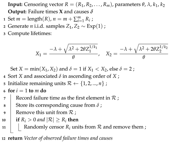
In this study, we consider CRs data under PT-IIRC. The progressively Type-II right-censored sample can be described as follows: Consider a life-testing experiment in which n units are placed under observation following a predefined progressive censoring scheme, denoted by $(R_1,R_2,\dots ,R_m)$. Assume that there are M independent causes of failure that are known. The number of observed failure times, denoted by m, is predetermined such that $1\le m\le n$.

At the time of the first observed failure, the $R_1$ units are removed from the remaining $n-1$ units. Subsequently, upon the occurrence of the second failure, additional $R_2$ units are withdrawn from the remaining $n-2-R_1$ units. This process continues iteratively until the occurrence of the $m^{th}$ failure. At this stage, denoted as $X_m$, all remaining surviving units are removed from the experiment, marking its termination. The progressive censoring scheme $(R_1,R_2,\dots ,R_m)$ must satisfy the following constraint:

$$\sum _{i=1}^m{R}_i=n-m.$$

• If $R_1=R_2=\cdots =R_{m-1}=0$, then the last removal is given by $R_m=n-m$, which reduces the setup to the conventional Type-II right censoring scheme.
• If $R_1=R_2=\cdots =R_m=0$, then $n=m$, which corresponds to a complete sample.

For a comprehensive discussion on progressive censoring schemes, refer to [29].

The primary goal of this study is to deliver the first comprehensive treatment of the GLE CRs model under the PT-IIRC pattern that arises routinely in long-term biomedical, biological, and industrial reliability studies. Integrating PT-IIRC with a parametric CRs framework goes beyond mathematical elegance: it mirrors real-world data collection practice, yields more efficient estimators, permits cost sensitive experimental designs, and provides a common analytic language across disparate application domains. Because progressive censoring records additional early and mid-time information, coupling it with the flexible GLE CRs model improves the identifiability of contrasting cause-specific hazard shapes. Moreover, in CRs settings, the withdrawal process may act preferentially on a single cause (e.g., patients removed owing to drug toxicity or machines retired by policy). The parametric formulation adopted here allows for formal testing of whether removal rates differ by latent cause, thereby strengthening validity checks and inference.

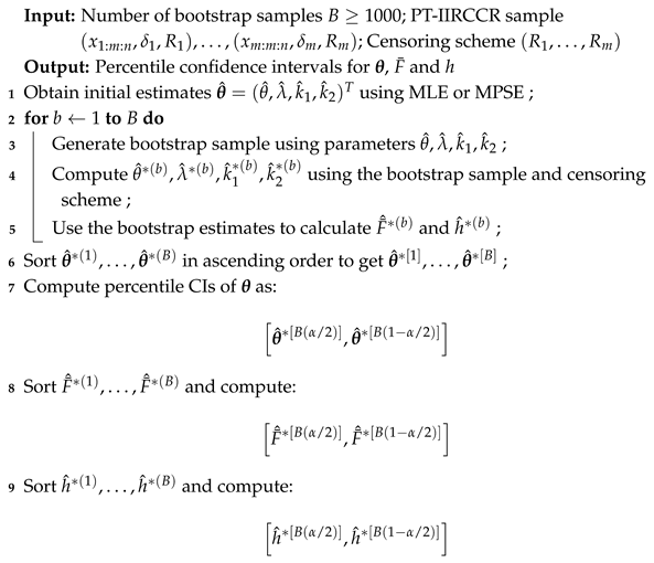
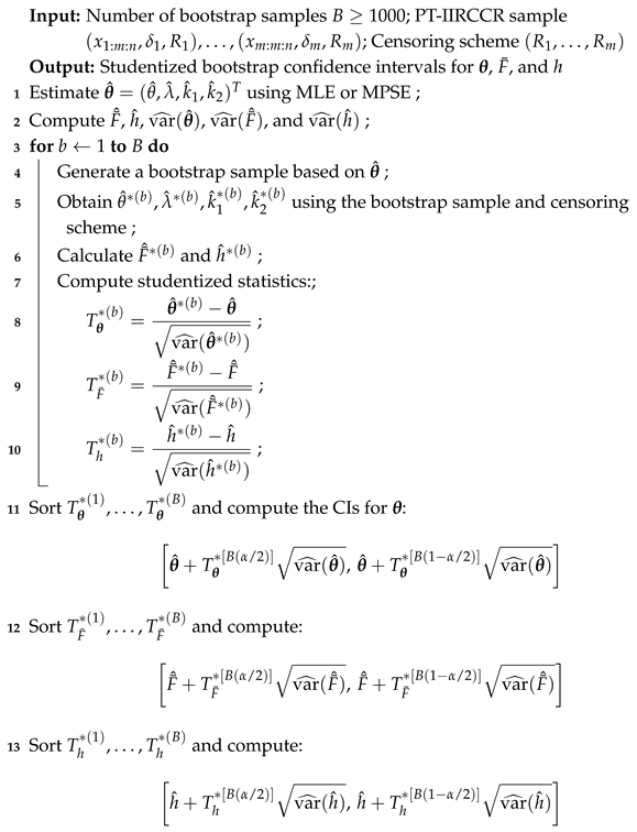
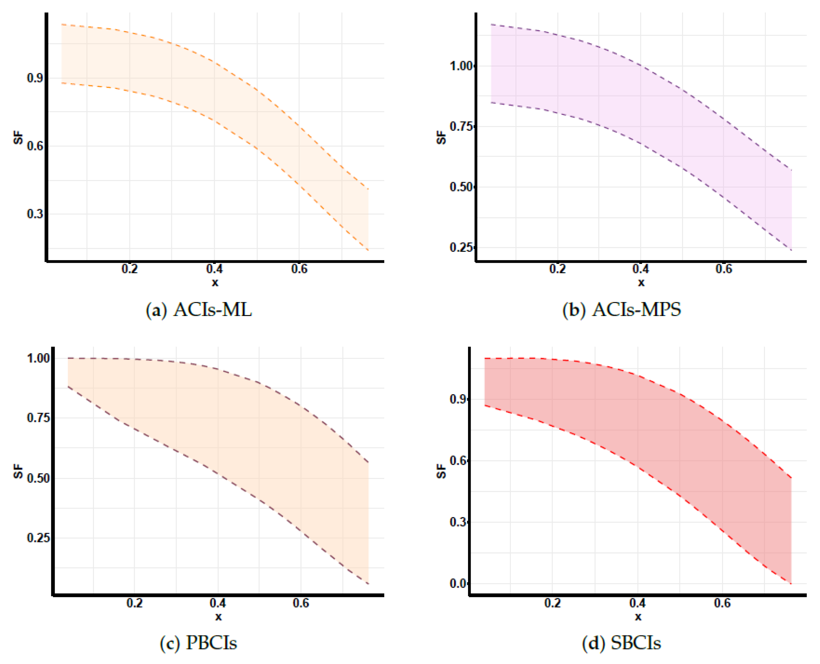
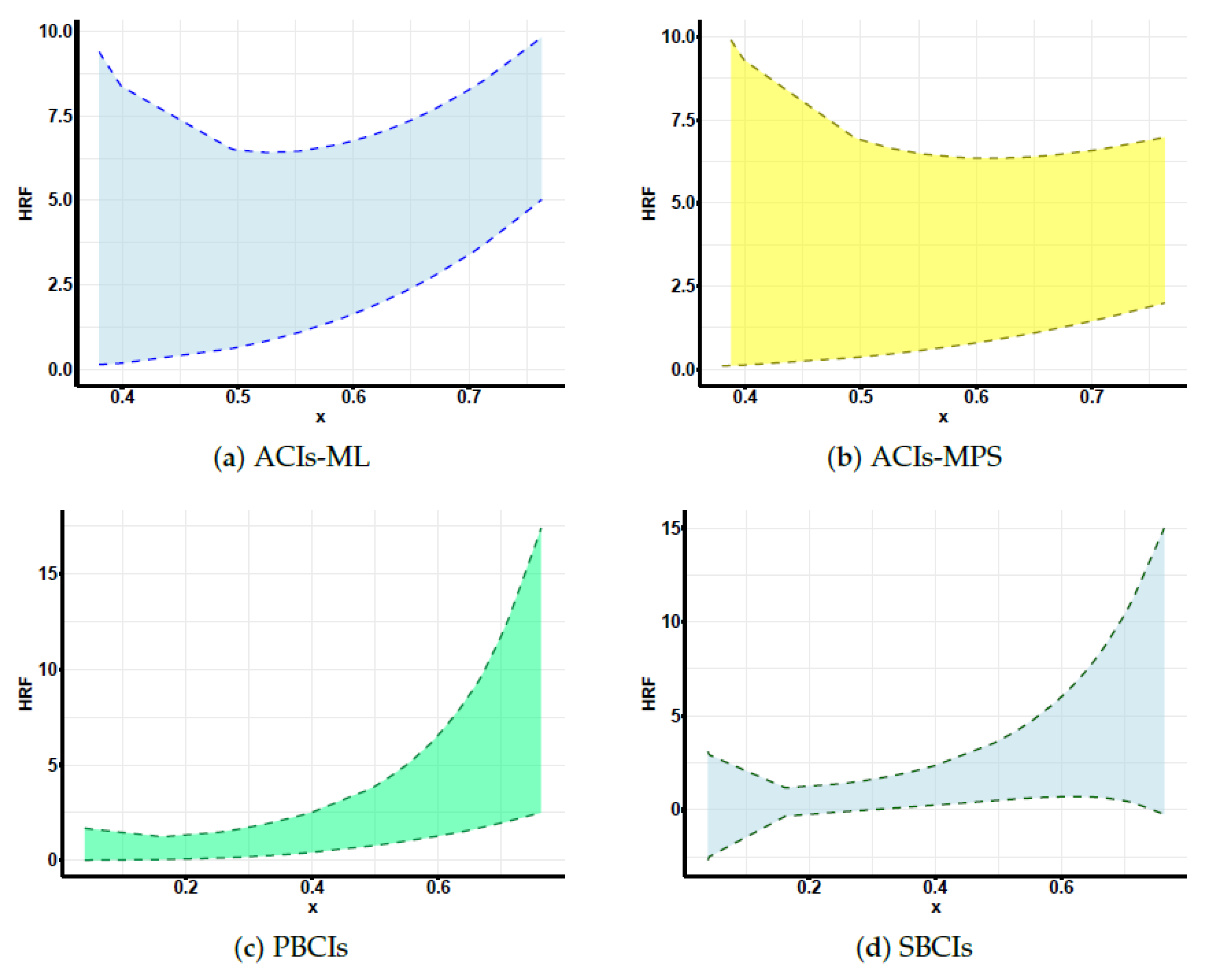
Developing maximum likelihood estimators (MLEs) and maximum product of spacing estimators (MPSEs): In addition, three distinct types of confidence intervals are developed: asymptotic confidence intervals (ACIs), percentile bootstrap confidence intervals (PBCIs), and studentized bootstrap confidence intervals (SBCIs). A Monte Carlo simulation is performed to evaluate and contrast the effectiveness of the proposed methods. Lastly, the proposed methods are applied to two real-world datasets for validation, with all analyses and computations performed using the R programming language to ensure accurate and efficient statistical processing.

The structure of the paper is as follows. Section 2 provides a detailed description of the model and introduces the necessary notation. The maximum likelihood estimation of unknown parameters is discussed in Section 3. Section 4 presents the maximum product of spacing estimation method and its theoretical foundations. Section 5 introduces the construction of bootstrap confidence intervals. 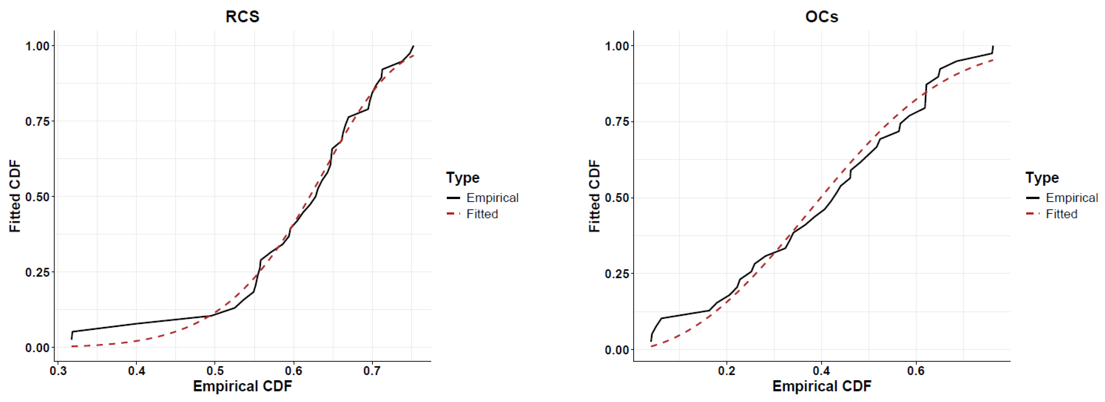A simulation study, along with its results and performance evaluation, is provided in Section 6. 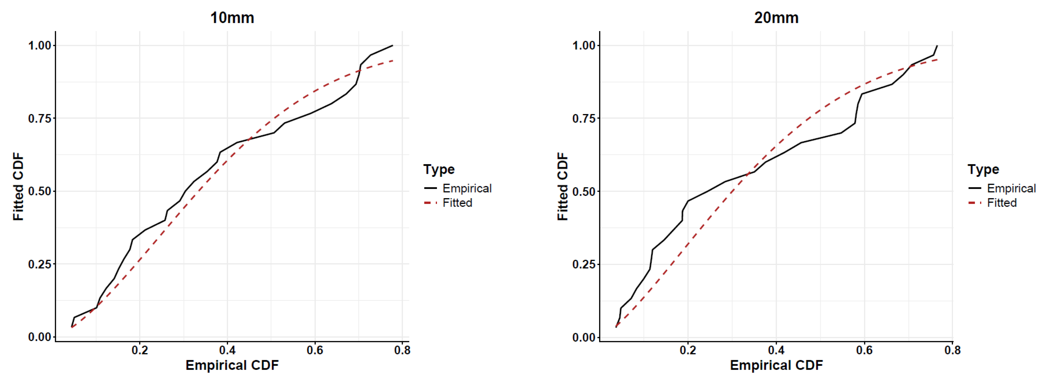In Section 7, real-world datasets are analyzed to illustrate the practical applicability of the proposed methods. Finally, the study concludes with a summary of findings and potential future research directions in Section 8.

2. Model Description and Notation

Consider a system with two independent failure causes ($M=2$). Let $X_{1i}$ and $X_{2i}$ ($i=1,\dots ,n$) represent the latent failure times associated with the two failure causes. Assume that these failure times are independent and identically distributed GLE distributions. Here, $X_{ji}$ represents the latent failure time of the $i\mathrm{th}$ unit that corresponds to the cause of failure $j\mathrm{th}$, where $j=1,2$.

Each failure in the experiment can occur due to one of $j(1\le j\le M)$ distinct causes. The failure mechanism is characterized as follows:

• m represents the total number of observed failures.
• $n-m$ denotes the total number of censored units.
• The cause of the failure is identified using an indicator variable ${\delta }_i$, where ${\delta }_i=j$ if the failure of $i\mathrm{th}$ is attributed to the risk of $j\mathrm{th}$.

Thus, the number of observed failures associated with the $j\mathrm{th}$ risk, denoted as $m_j$, is given by

$$m_1=\sum _{i=1}^{m}I({\delta }_i=1)\mathrm{and}{m}_2=\sum _{i=1}^{m}I({\delta }_i=2)$$

where $m=m_1+m_2$, and $I({\delta }_i=j)$ is an indicator function defined as

$$I({\delta }_i=j)=\left\{\begin{array}{cc}1,\hfill & \mathrm{if}{\delta }_i=j,\hfill \\ 0,\hfill & \mathrm{otherwise}.\hfill \end{array}\right.$$

The progressive Type-II censored CRs (PT-IIRCCR) data structure is represented as

$$(X_{1:m:n},{\delta }_1,R_1),\dots ,(X_{m:m:n},{\delta }_m,R_m)$$

where

• $X_{1:m:n}<\cdots <X_{m:m:n}$ denote the observed failure times.
• ${\delta }_1,{\delta }_2,\dots ,{\delta }_m$ represent the corresponding causes of failure.
• $R_1,R_2,\dots ,R_m$ indicate the number of units removed from the experiment at each observed failure time.

Several special cases of this censoring mechanism warrant further discussion.

Under these assumptions, the survival function (SF) of $X_{ji}$ is expressed as

$$\overline{F_j}(x;\mathit{\theta })=exp\left[-{\left({\displaystyle \frac{\theta }{2}}{x}^2+\lambda x\right)}^{k_j}\right];x>0,\theta ,k_j>0,\lambda \ge 0.$$

(1)

The cumulative distribution function (CDF) and the probability density function (PDF) of $X_{ji}$ are expressed as follows:

$$F_j(x;\mathit{\theta })=1-exp\left[-{\left({\displaystyle \frac{\theta }{2}}{x}^2+\lambda x\right)}^{k_j}\right];x>0,\theta ,k_j>0,\lambda \ge 0$$

(2)

and its PDF is

$$f_j(x;\mathit{\theta })=k_j(\theta x+\lambda ){\left({\displaystyle \frac{\theta }{2}}{x}^2+\lambda x\right)}^{k_j-1}exp\left[-{\left({\displaystyle \frac{\theta }{2}}{x}^2+\lambda x\right)}^{k_j}\right];x>0,\theta ,k_j>0,\lambda \ge 0.$$

(3)

The hazard rate function (HRF) is given by

$$h_j(x;\mathit{\theta })=k_j(\theta x+\lambda ){\left({\displaystyle \frac{\theta }{2}}{x}^2+\lambda x\right)}^{k_j-1};x>0,\theta ,k_j>0,\lambda \ge 0.$$

(4)

Consider a reliability study involving identical n units in a lifetime experiment, where each unit may fail due to one of two competing causes. The observed failure time for the $i\mathrm{th}$ unit is given by

$$X_i=min(X_{i1},X_{i2}),i=1,\dots ,n.$$

Using Equations (2) and (3), the CDF and PDF of $X_i$ can be derived as follows:

$$F(x;\mathit{\theta })=1-exp\left[-\sum _{j=1}^2{\left({\displaystyle \frac{\theta }{2}}{x}^2+\lambda x\right)}^{k_j}\right];x>0$$

(5)

and

$$f(x;\mathit{\theta })=(\theta x+\lambda )\left[\sum _{j=1}^2{k}_j{\left({\displaystyle \frac{\theta }{2}}{x}^2+\lambda x\right)}^{k_j-1}\right]exp\left[-\sum _{j=1}^2{\left({\displaystyle \frac{\theta }{2}}{x}^2+\lambda x\right)}^{k_j}\right];x>0$$

(6)

where $\mathit{\theta }$ represents the vector of model parameters, which is defined within the parameter space $\mathit{\Theta }$, that is,

$$\mathit{\theta }={(\theta ,\lambda ,k_1,k_2)}^T\in {\mathbb{R}}_{+}^4\cup \{\lambda =0\}.$$

In the same way, the SF and HRF of $X_i$ can be expressed as follows:

$$\overline{F}(x;\mathit{\theta })=exp\left[-\sum _{j=1}^2{\left({\displaystyle \frac{\theta }{2}}{x}^2+\lambda x\right)}^{k_j}\right];x>0$$

(7)

and

$$h(x;\mathit{\theta })=(\theta x+\lambda )\left[\sum _{j=1}^2{k}_j{\left({\displaystyle \frac{\theta }{2}}{x}^2+\lambda x\right)}^{k_j-1}\right];x>0.$$

(8)

All items under study undergo similar conditions, whether patients or engineered components operate in the same external environment and are exposed to similar baseline stresses (temperature, workload, treatment protocol, etc.). We therefore adopt the rate parameters $\lambda$ and an acceleration term $\theta$ that apply uniformly to every latent failure time. The different physical or biological mechanisms of failure are instead represented by the shape parameters $k_1$ and $k_2$. Hence, the parsimonious four-parameter specification achieves better numerical stability and provides a clearer, mechanism-oriented interpretation.

3. The Maximum Likelihood Estimation

The maximum likelihood estimation (MLE) method is widely used for parameter estimation due to its advantageous properties, including consistency, asymptotic normality, invariance, and asymptotic efficiency. In addition, it often exhibits favorable convergence behavior; see [30]. The large sample properties of MLE, particularly, strong consistency and asymptotic normality, have also been rigorously examined in [31].

Based on the previous discussion, we can derive the joint likelihood function for the GLE CRs model under the PT-IIRC condition for the observed dataset m, represented as $(X_{i:m:n};{\delta }_i,R_i)$, where ${\delta }_i\in \{1,2\}$ for $i=1,2,\dots ,m$. Here, ${\delta }_i=1$ indicates that the failure of the item $i^{th}$ is attributed to the first cause, while ${\delta }_i=2$ means that the failure is due to the second cause. The joint likelihood function is formulated as follows:

$$\begin{array}{cc}\hfill L(\mathit{\theta }\mid \mathbf{x})& =C\prod _{i=1}^m{\left[f_1\left(x_{i:m:n}\right){\overline{F}}_2\left(x_{i:m:n}\right)\right]}^{I({\delta }_i=1)}{\left[f_2\left(x_{i:m:n}\right){\overline{F}}_1\left(x_{i:m:n}\right)\right]}^{I({\delta }_i=2)}\hfill \\ \hfill & \times {\left[{\overline{F}}_1\left(x_{i:m:n}\right){\overline{F}}_2\left(x_{i:m:n}\right)\right]}^{R_i}\hfill \end{array}$$

(9)

where

$$C=n\prod _{i=1}^{m-1}\left[n-\sum _{\tau =1}^i(R_{\tau }+1)\right].$$

Another form of the likelihood function in (9) can be obtained using the identity $f_j\left(x\right)=h_j\left(x\right){\overline{F}}_j\left(x\right)$ as follows:

$$L(\mathit{\theta }\mid \mathbf{x})=C\prod _{i=1}^m{\left[h_1\left(x_i\right)\right]}^{I({\delta }_i=1)}{\left[h_2\left(x_i\right)\right]}^{I({\delta }_i=2)}{\left[{\overline{F}}_1\left(x_i\right){\overline{F}}_2\left(x_i\right)\right]}^{1+R_i}$$

(10)

where $h_j\left(x\right)=f_j\left(x\right)/{\overline{F}}_j\left(x\right)$, $j=1,2$, and $x_i=x_{i:m:n}$ for simplicity of notation.

3.1. Point Estimation

By substituting (4) and (1) into (10), the joint likelihood function of $\mathit{\theta }$ is expressed as

$$\begin{array}{cc}\hfill L(\mathit{\theta }\mid \mathbf{x})& =C\prod _{i=1}^{m_1}{k}_1{\eta }^{\prime }(x_i;\theta ,\lambda ){\eta }^{k_1-1}(x_i;\theta ,\lambda )\prod _{i=1}^{m_2}{k}_2{\eta }^{\prime }(x_i;\theta ,\lambda ){\eta }^{k_2-1}(x_i;\theta ,\lambda )\hfill \\ \hfill & \times \prod _{i=1}^{m}exp\left[-(1+R_i)\sum _{j=1}^2{\eta }^{k_j}(x_i;\theta ,\lambda )\right]\hfill \end{array}$$

(11)

where $\eta (x_i;\theta ,\lambda )={\displaystyle \frac{\theta }{2}}{x}_i^2+\lambda x_i,$ and ${\eta }^{\prime }(x_i;\theta ,\lambda )=\theta x_i+\lambda$. Equation (11) can be rewritten in a simplified form as

$$L(\mathit{\theta }\mid \mathbf{x})=C\prod _{j=1}^2\prod _{i=1}^{m_j}{k}_j{\eta }^{k_j-1}(x_i;\theta ,\lambda )\prod _{i=1}^m{\eta }^{\prime }(x_i;\theta ,\lambda )exp\left[-(1+R_i)\sum _{j=1}^2{\eta }^{k_j}(x_i;\theta ,\lambda )\right].$$

(12)

Taking the logarithm of (12), excluding the constant term, results in the following:

$$\begin{array}{cc}\hfill \ell (\mathit{\theta }\mid \mathbf{x})& \propto \sum _{j=1}^2{m}_{j}log\left(k_j\right)+\sum _{i=1}^{m}log{\eta }^{\prime }(x_i;\theta ,\lambda )+\sum _{j=1}^2\sum _{i=1}^{m_j}(k_j-1)log\eta (x_i;\theta ,\lambda )\hfill \\ \hfill & -\sum _{j=1}^2\sum _{i=1}^m(1+R_i){\left[\eta (x_i;\theta ,\lambda )\right]}^{k_j}\hfill \end{array}$$

(13)

where $\mathit{\theta }={(\theta ,\lambda ,k_1,k_2)}^T$. MLEs are obtained by maximizing the log-likelihood function in (13) with respect to its parameters. Alternatively, these estimates can be derived by computing the first-order partial derivatives of (13), equating them to zero, and solving the resulting normal equations. The MLEs, denoted by $\widehat{\theta },\widehat{\lambda },{\widehat{k}}_j$ for $j=1,2$, are then determined by solving these equations simultaneously.

$${\displaystyle \frac{\partial \ell }{\partial \theta }}=\sum _{i=1}^m{\displaystyle \frac{x_i}{{\eta }^{\prime }(x_i;\theta ,\lambda )}}+\sum _{j=1}^2\sum _{i=1}^{m_j}{\displaystyle \frac{(k_j-1)x_i^2}{2\eta (x_i;\theta ,\lambda )}}-\sum _{j=1}^2\sum _{i=1}^m{k}_j(1+R_i){\displaystyle \frac{x_i^2}{2}}{\eta }^{k_j-1}(x_i;\theta ,\lambda )=0,$$

(14)

$${\displaystyle \frac{\partial \ell }{\partial \lambda }}=\sum _{i=1}^m{\displaystyle \frac{1}{{\eta }^{\prime }(x_i;\theta ,\lambda )}}+\sum _{j=1}^2\sum _{i=1}^{m_j}{\displaystyle \frac{(k_j-1)x_i}{\eta (x_i;\theta ,\lambda )}}-\sum _{j=1}^2\sum _{i=1}^m{k}_j(1+R_i)x_i{\eta }^{k_j-1}(x_i;\theta ,\lambda )=0$$

(15)

and

$${\displaystyle \frac{\partial \ell }{\partial k_j}}={\displaystyle \frac{m_j}{k_j}}+\sum _{i=1}^{m_j}log\eta (x_i;\theta ,\lambda )-\sum _{i=1}^m(1+R_i){\eta }^{k_j}(x_i;\theta ,\lambda )log\eta (x_i;\theta ,\lambda )=0,j=1,2.$$

(16)

Due to the complex forms of (14), (15), and (16), the MLEs cannot be derived explicitly. Consequently, numerical iterative methods are required to compute the desired estimates.

Furthermore, leveraging the invariance property of MLEs, the estimates for the SF and HRF can be directly obtained from (7) and (8), respectively, as follows:

$$\widehat{\overline{F}}\left(x\right)=exp\left[-\sum _{j=1}^2{\left({\displaystyle \frac{\widehat{\theta }}{2}}{x}^2+\widehat{\lambda }x\right)}^{{\widehat{k}}_j}\right];x>0$$

(17)

and

$$\widehat{h}\left(x\right)=(\widehat{\theta }x+\widehat{\lambda })\sum _{j=1}^2{\widehat{k}}_j{\left({\displaystyle \frac{\widehat{\theta }}{2}}{x}^2+\widehat{\lambda }x\right)}^{{\widehat{k}}_j-1};x>0.$$

(18)

3.2. ACIs Using MLEs

The ACIs for unknown parameters $\theta ,\lambda ,k_1$, and $k_2$, as well as for the SF and HRF, are developed based on the asymptotic normality property of the MLE. Using the log-likelihood function in (13), the observed Fisher information matrix $I_{obs}\left(\mathit{\theta }\right)$ is defined as

$$I_{obs}\left(\mathit{\theta }\right)={\left[-{\displaystyle \frac{{\partial }^2\ell \left(\mathit{\theta }\right)}{\partial {\mathit{\theta }}_r\partial {\mathit{\theta }}_s}}\right]}_{\mathit{\theta }=\widehat{\mathit{\theta }}},r,s=1,2,3,4$$

(19)

where the second derivatives ${\displaystyle \frac{{\partial }^2\ell \left(\mathit{\theta }\right)}{\partial {\mathit{\theta }}_r\partial {\mathit{\theta }}_s}}$, $r,s=1,2,3,4$, are given by

$${\displaystyle \frac{{\partial }^2\ell }{\partial {\theta }^2}}=-\sum _{i=1}^m{\displaystyle \frac{x_i^2}{{\eta }^{\prime 2}(x_i;\theta ,\lambda )}}-\sum _{j=1}^2\sum _{i=1}^{m_j}{\displaystyle \frac{(k_j-1)x_i^4}{4{\eta }^2(x_i;\theta ,\lambda )}}-\sum _{j=1}^2\sum _{i=1}^m{k}_j(k_j-1)(1+R_i){\displaystyle \frac{x_i^4}{4}}{\eta }^{k_j-2}(x_i;\theta ,\lambda ),$$

(20)

$$\begin{array}{cc}\hfill {\displaystyle \frac{{\partial }^2\ell }{\partial \theta \partial \lambda }}={\displaystyle \frac{{\partial }^2\ell }{\partial \lambda \partial \theta }}& =-\sum _{i=1}^m{\displaystyle \frac{x_i}{{\eta }^{\prime 2}(x_i;\theta ,\lambda )}}-\sum _{j=1}^2\sum _{i=1}^{m_j}{\displaystyle \frac{(k_j-1)x_i^3}{2{\eta }^2(x_i;\theta ,\lambda )}}\hfill \\ \hfill & -\sum _{j=1}^2\sum _{i=1}^m{k}_j(k_j-1)(1+R_i){\displaystyle \frac{x_i^3}{2}}{\eta }^{k_j-2}(x_i;\theta ,\lambda ),\hfill \end{array}$$

(21)

$$\begin{array}{cc}\hfill {\displaystyle \frac{{\partial }^2\ell }{\partial \theta \partial k_j}}={\displaystyle \frac{{\partial }^2\ell }{\partial k_j\partial \theta }}& =\sum _{i=1}^{m_j}{\displaystyle \frac{x_i^2}{2\eta (x_i;\theta ,\lambda )}}-\sum _{i=1}^{m_j}(1+R_i){\displaystyle \frac{x_i^2}{2}}{\eta }^{k_j-1}(x_i;\theta ,\lambda )\hfill \\ \hfill & -\sum _{i=1}^m{k}_j(1+R_i){\displaystyle \frac{x_i^2}{2}}{\eta }^{k_j-1}(x_i;\theta ,\lambda )log\eta (x_i;\theta ,\lambda ),\hfill \end{array}$$

(22)

$${\displaystyle \frac{{\partial }^2\ell }{\partial {\lambda }^2}}=-\sum _{i=1}^m{\displaystyle \frac{1}{{\eta }^{\prime 2}(x_i;\theta ,\lambda )}}-\sum _{j=1}^2\sum _{i=1}^{m_j}{\displaystyle \frac{(k_j-1)x_i^2}{{\eta }^2(x_i;\theta ,\lambda )}}-\sum _{j=1}^2\sum _{i=1}^m{k}_j(k_j-1)(1+R_i)x_i^2{\eta }^{k_j-2}(x_i;\theta ,\lambda ),$$

(23)

$$\begin{array}{cc}\hfill {\displaystyle \frac{{\partial }^2\ell }{\partial \lambda \partial k_j}}={\displaystyle \frac{{\partial }^2\ell }{\partial k_j\partial \lambda }}& =\sum _{i=1}^{m_j}{\displaystyle \frac{x_i}{\eta (x_i;\theta ,\lambda )}}-\sum _{i=1}^{m_j}(1+R_i)x_i{\eta }^{k_j-1}(x_i;\theta ,\lambda )\hfill \\ \hfill & -\sum _{i=1}^m{k}_j{x}_i(1+R_i){\eta }^{k_j-1}(x_i;\theta ,\lambda )log\eta (x_i;\theta ,\lambda )\hfill \end{array}$$

(24)

and

$$\begin{array}{cc}\hfill {\displaystyle \frac{{\partial }^2\ell }{\partial k_j^2}}& =-{\displaystyle \frac{m_j}{k_j^2}}-\sum _{i=1}^m(1+R_i){\eta }^{k_j}(x_i;\theta ,\lambda ){\left[log\eta (x_i;\theta ,\lambda )\right]}^2.\hfill \end{array}$$

(25)

According to [32], the asymptotic normality of the MLEs based on PT-IIRC samples is established under specific regularity conditions. As the sample size increases, the MLEs approach a normal distribution asymptotically. Consequently, the asymptotic distribution of the parameters $\theta ,\lambda ,k_1$, and $k_2$ can be expressed as

$$(\widehat{\theta },\widehat{\lambda },{\widehat{k}}_1,{\widehat{k}}_2)\sim N_4\left[(\theta ,\lambda ,k_1,k_2),I(\widehat{\theta },\widehat{\lambda },{\widehat{k}}_1,{\widehat{k}}_2)\right],$$

where $I(\widehat{\theta },\widehat{\lambda },{\widehat{k}}_1,{\widehat{k}}_2)$ is the asymptotic variance–covariance matrix of $\widehat{\mathit{\theta }}$. It can be approximated by taking the inverse of (19), thus giving

$$I\left(\widehat{\mathit{\theta }}\right)=I(\widehat{\theta },\widehat{\lambda },{\widehat{k}}_1,{\widehat{k}}_2)=\left[\begin{array}{cccc}\widehat{var}\left(\widehat{\theta }\right)& \widehat{cov}(\widehat{\theta },\widehat{\lambda })& \widehat{cov}(\widehat{\theta },{\widehat{k}}_1)& \widehat{cov}(\widehat{\theta },{\widehat{k}}_2)\\ \widehat{cov}(\widehat{\lambda },\widehat{\theta })& \widehat{var}\left(\widehat{\lambda }\right)& \widehat{cov}(\widehat{\lambda },{\widehat{k}}_1)& \widehat{cov}(\widehat{\lambda },{\widehat{k}}_2)\\ \widehat{cov}({\widehat{k}}_1,\widehat{\theta })& \widehat{cov}({\widehat{k}}_1,\widehat{\lambda })& \widehat{var}\left({\widehat{k}}_1\right)& \widehat{cov}({\widehat{k}}_1,{\widehat{k}}_2)\\ \widehat{cov}({\widehat{k}}_2,\widehat{\theta })& \widehat{cov}({\widehat{k}}_2,\widehat{\lambda })& \widehat{cov}({\widehat{k}}_2,{\widehat{k}}_1)& \widehat{var}\left({\widehat{k}}_2\right)\end{array}\right].$$

(26)

Hence, the two-sided ACIs $100(1-\alpha )\%$ for the parameters $\theta ,\lambda ,k_1$, and $k_2$ are as follows:

$$\begin{gathered} \left[\widehat{\theta }\pm z_{\alpha /2}\sqrt{\widehat{var}\left(\widehat{\theta }\right)}\right],\left[\widehat{\lambda }\pm z_{\alpha /2}\sqrt{\widehat{var}\left(\widehat{\lambda }\right)}\right], \\ \left[{\widehat{k}}_1\pm z_{\alpha /2}\sqrt{\widehat{var}\left({\widehat{k}}_1\right)}\right]\mathrm{and}\left[{\widehat{k}}_2\pm z_{\alpha /2}\sqrt{\widehat{var}\left({\widehat{k}}_2\right)}\right] \end{gathered}$$

where $z_{\alpha /2}$ is the upper $\alpha /2$ percentile of the standard normal distribution.

3.3. ACIs for SF and HRF

To construct the ACIs for the SF and HRF, it is necessary to determine the variances of their corresponding MLEs. In this context, the delta method is employed to approximate the variances of $\widehat{\overline{F}}\left(x\right)$ and $\widehat{h}\left(x\right)$. For the application of this approach, let ${\Psi }_1$ and ${\Psi }_2$ represent two quantities defined as follows:

$${\Psi }_1=\left[{\displaystyle \frac{\partial \overline{F}\left(x\right)}{\partial \theta }},{\displaystyle \frac{\partial \overline{F}\left(x\right)}{\partial \lambda }},{\displaystyle \frac{\partial \overline{F}\left(x\right)}{\partial k_1}},{\displaystyle \frac{\partial \overline{F}\left(x\right)}{\partial k_2}}\right]\mathrm{and}{\Psi }_2=\left[{\displaystyle \frac{\partial h\left(x\right)}{\partial \theta }},{\displaystyle \frac{\partial h\left(x\right)}{\partial \lambda }},{\displaystyle \frac{\partial h\left(x\right)}{\partial k_1}},{\displaystyle \frac{\partial h\left(x\right)}{\partial k_2}}\right]$$

where

$${\displaystyle \frac{\partial \overline{F}\left(x\right)}{\partial \theta }}=-{\displaystyle \frac{x^2}{2}}\sum _{j=1}^2{k}_j{\eta }^{k_j-1}(x;\theta ,\lambda )exp[-\sum _{j=1}^2{\eta }^{k_j}(x;\theta ,\lambda )],$$

(27)

$${\displaystyle \frac{\partial \overline{F}\left(x\right)}{\partial \lambda }}=-x\sum _{j=1}^2{k}_j{\eta }^{k_j-1}(x;\theta ,\lambda )exp[-\sum _{j=1}^2{\eta }^{k_j}(x;\theta ,\lambda )],$$

(28)

$${\displaystyle \frac{\partial \overline{F}\left(x\right)}{\partial k_j}}=-{\eta }^{k_j}(x;\theta ,\lambda )log\eta (x_i;\theta ,\lambda )exp[-\sum _{j=1}^2{\eta }^{k_j}(x;\theta ,\lambda )],$$

(29)

$${\displaystyle \frac{\partial h\left(x\right)}{\partial \theta }}=x\sum _{j=1}^2{k}_j{\eta }^{k_j-1}(x;\theta ,\lambda )+{\displaystyle \frac{{\eta }^{\prime }(x;\theta ,\lambda )}{2}}\sum _{j=1}^2{k}_j(k_j-1)x^2{\eta }^{k_j-2}(x;\theta ,\lambda ),$$

(30)

$${\displaystyle \frac{\partial h\left(x\right)}{\partial \lambda }}=\sum _{j=1}^2{k}_j{\eta }^{k_j-1}(x;\theta ,\lambda )+{\eta }^{\prime }(x;\theta ,\lambda )\sum _{j=1}^2{k}_j(k_j-1)x{\eta }^{k_j-2}(x;\theta ,\lambda )$$

(31)

and

$${\displaystyle \frac{\partial h\left(x\right)}{\partial k_j}}={\eta }^{\prime }(x;\theta ,\lambda ){\eta }^{k_j-1}(x;\theta ,\lambda )\left[1+k_{j}log\eta (x;\theta ,\lambda )\right].$$

(32)

Consequently, the approximate variance estimates for the SF and HRF can be expressed, respectively, as follows:

$$\widehat{var}\left(\widehat{\overline{F}}\right)=\left[{\Psi }_{1}I\left(\widehat{\mathit{\theta }}\right){\Psi }_1^T\right]{|}_{(\mathit{\theta }=\widehat{\mathit{\theta }})} \mathrm{and} \widehat{var}\left(\widehat{h}\right)=\left[{\Psi }_{2}I\left(\widehat{\mathit{\theta }}\right){\Psi }_2^T\right]{|}_{(\mathit{\theta }=\widehat{\mathit{\theta }})}$$

where $I\left(\widehat{\mathit{\theta }}\right)$ is given by (26). Thus,

$${\displaystyle \frac{\widehat{\overline{F}}\left(x\right)-\overline{F}\left(x\right)}{\sqrt{\widehat{var}\left(\widehat{\overline{F}}\right)}}}\sim SN(0,1) \mathrm{and} {\displaystyle \frac{\widehat{h}\left(x\right)-h\left(x\right)}{\sqrt{\widehat{var}\left(\widehat{h}\right)}}}\sim SN(0,1),$$

asymptotically. Then, the $100(1-\alpha )\%$ ACIs of $\overline{F}\left(x\right)$ and $h\left(x\right)$ are, respectively, defined as follows:

$$\left[\widehat{\overline{F}}\pm z_{\alpha /2}\sqrt{\widehat{var}\left(\widehat{\overline{F}}\right)}\right] \mathrm{and} \left[\widehat{h}\pm z_{\alpha /2}\sqrt{\widehat{var}\left(\widehat{h}\right)}\right].$$

The lower bounds of the ACIs computed using the previous approach may occasionally yield negative values. To address this issue, the delta method, as described in [33], can be applied to obtain the ACIs. In this case, the distribution of $log\widehat{\zeta }$ can be approximated by

$$Z_{log\widehat{\zeta }}={\displaystyle \frac{log\widehat{\zeta }-log\zeta }{\widehat{var}(log\widehat{\zeta })}}\sim SN(0,1)$$

where $\widehat{var}(log\widehat{\zeta })$ can be derived using the delta method as

$$\widehat{var}(log\widehat{\zeta })={\displaystyle \frac{\widehat{var}\left(\widehat{\zeta }\right)}{{\widehat{\zeta }}^2}}.$$

As a result, the two-sided $100(1-\alpha )\%$ normal ACIs for a positive parameter can be formulated as

$$\left\{\widehat{\zeta }exp\left[-{\displaystyle \frac{z_{1-\alpha /2}\sqrt{\widehat{var}\left(\widehat{\zeta }\right)}}{\widehat{\zeta }}}\right],\widehat{\zeta }exp\left[{\displaystyle \frac{z_{1-\alpha /2}\sqrt{\widehat{var}\left(\widehat{\zeta }\right)}}{\widehat{\zeta }}}\right]\right\}$$

where $\widehat{\zeta }$ represents the maximum likelihood estimator of the parameter vector, i.e.,

$$\widehat{\zeta }=(\widehat{\theta },\widehat{\lambda },{\widehat{k}}_1,{\widehat{k}}_2,\widehat{\overline{F}}\left(x\right),\widehat{h}\left(x\right)),$$

and $\widehat{var}\left(\widehat{\zeta }\right)$ denotes its corresponding asymptotic variance.

4. The Maximum Product of Spacing Estimation

Ref. [34] proposed the maximum product of spacing estimation (MPSE) method as a general approach to estimating parameters in continuous univariate distributions, particularly when one parameter represents a shifted origin. The MPSEs retain several desirable properties of the MLEs, including consistency, asymptotic normality, and the invariance property. Furthermore, Ref. [35] extended the MPSE method approach to handle parameter estimation based on PT-IIRC samples. The MPSE method identifies the parameter values that render the observed data as uniformly distributed as possible according to a specific quantitative measure of uniformity.

4.1. Point Estimation

Let $D_{ji}\left(\mathit{\theta }\right)=F_j(x_{i:m:n};\mathit{\theta })-F_j(x_{i-1:m:n};\mathit{\theta })$, for $j=1,2$ and $i=1,2,\dots ,m+1$, represent a uniform spacing, where $F(x_{0:m:n};\mathit{\theta })=0$, and $F(x_{m+1:m:n};\mathit{\theta })=1$. It is evident that ${\sum }_{i=1}^{m+1}{D}_i\left(\mathit{\theta }\right)=1$.

For the CRs model, under the framework of PT-IIRC data, the product of spacings that needs to be maximized is given by

$$P\left(\mathit{\theta }\right)=\prod _{i=1}^{m+1}{\left[D_{1i}{\overline{F}}_2\left(x_{i:m:n}\right)\right]}^{I({\delta }_i=1)}{\left[D_{2i}{\overline{F}}_1\left(x_{i:m:n}\right)\right]}^{I({\delta }_i=2)}\prod _{i=1}^m{\left[{\overline{F}}_1\left(x_{i:m:n}\right){\overline{F}}_2\left(x_{i:m:n}\right)\right]}^{R_i}.$$

(33)

Equation (33) can be rewritten in the following form:

$$P\left(\mathit{\theta }\right)=\prod _{j=1}^2\prod _{i=1}^{m_j+1}\left[{\displaystyle \frac{{\overline{F}}_j\left(x_{i-1:m:n}\right)}{{\overline{F}}_j\left(x_{i:m:n}\right)}}-1\right]\prod _{i=1}^m{\left[{\overline{F}}_1\left(x_{i:m:n}\right){\overline{F}}_2\left(x_{i:m:n}\right)\right]}^{R_i+1}.$$

(34)

By substituting (1) into (34), we obtain

$$P\left(\mathit{\theta }\right)=\prod _{j=1}^2\prod _{i=1}^{m_j+1}\left[e^{{\eta }^{k_j}(x_{i:m:n};\theta ,\lambda )-{\eta }^{k_j}(x_{i-1:m:n};\theta ,\lambda )}-1\right]\prod _{i=1}^{m}exp\left[-(1+R_i)\sum _{j=1}^2{\eta }^{k_j}(x_{i:m:n};\theta ,\lambda )\right].$$

(35)

By taking the logarithm of (35), we get

$$logP\left(\mathit{\theta }\right)=\sum _{j=1}^2\sum _{i=1}^{m_j+1}log\left[e^{{\eta }^{k_j}(x_{i:m:n};\theta ,\lambda )-{\eta }^{k_j}(x_{i-1:m:n};\theta ,\lambda )}-1\right]-\sum _{j=1}^2\sum _{i=1}^m(1+R_i){\eta }^{k_j}(x_{i:m:n};\theta ,\lambda ).$$

(36)

The MPSEs of $\mathit{\theta }={(\theta ,\lambda ,k_1,k_2)}^T$, denoted by $\tilde{\theta },\tilde{\lambda },{\tilde{k}}_1$, and ${\tilde{k}}_2$, are obtained by maximizing (36) with respect to $\mathit{\theta }$. These estimators can be determined by simultaneously solving the following system of normal equations:

$${\displaystyle \frac{\partial logP}{\partial \theta }}=\sum _{j=1}^2\sum _{i=1}^{m_j+1}{\displaystyle \frac{e^{{\xi }_i}{\left({\xi }_i\right)}_{\theta }}{e^{{\xi }_i}-1}}-{\displaystyle \frac{1}{2}}\sum _{j=1}^2\sum _{i=1}^m(1+R_i)k_j{x}_{i:m:n}^2{\eta }^{k_j-1}(x_{i:m:n};\theta ,\lambda )=0,$$

(37)

$${\displaystyle \frac{\partial logP}{\partial \lambda }}=\sum _{j=1}^2\sum _{i=1}^{m_j+1}{\displaystyle \frac{e^{{\xi }_i}{\left({\xi }_i\right)}_{\lambda }}{e^{{\xi }_i}-1}}-\sum _{j=1}^2\sum _{i=1}^m(1+R_i)k_j{x}_{i:m:n}{\eta }^{k_j-1}(x_{i:m:n};\theta ,\lambda )=0$$

(38)

and

$${\displaystyle \frac{\partial logP}{\partial k_j}}=\sum _{i=1}^{m_j+1}{\displaystyle \frac{e^{{\xi }_i}{\left({\xi }_i\right)}_{k_j}}{e^{{\xi }_i}-1}}-\sum _{i=1}^m(1+R_i){\eta }^{k_j}(x_{i:m:n};\theta ,\lambda )log\eta (x_{i:m:n};\theta ,\lambda )=0$$

(39)

where ${\xi }_i={\xi }_i(\theta ,\lambda ,k_1,k_2)={\eta }^{k_j}(x_{i:m:n};\theta ,\lambda )-{\eta }^{k_j}(x_{i-1:m:n};\theta ,\lambda )$,

$$\begin{array}{cc}\hfill {\left({\xi }_i\right)}_{\theta }& ={\displaystyle \frac{\partial }{\partial \theta }}\left[{\eta }^{k_j}(x_{i:m:n};\theta ,\lambda )-{\eta }^{k_j}(x_{i-1:m:n};\theta ,\lambda )\right]\hfill \\ \hfill & ={\displaystyle \frac{k_j}{2}}\left[x_i^2{\eta }^{k_j-1}(x_{i:m:n};\theta ,\lambda )-x_{i-1}^2{\eta }^{k_j-1}(x_{i-1:m:n};\theta ,\lambda )\right],\hfill \end{array}$$

(40)

$$\begin{array}{cc}\hfill {\left({\xi }_i\right)}_{\lambda }& ={\displaystyle \frac{\partial }{\partial \lambda }}\left[{\eta }^{k_j}(x_{i:m:n};\theta ,\lambda )-{\eta }^{k_j}(x_{i-1:m:n};\theta ,\lambda )\right]\hfill \\ \hfill & =k_j\left[x_i{\eta }^{k_j-1}(x_{i:m:n};\theta ,\lambda )-x_{i-1}{\eta }^{k_j-1}(x_{i-1:m:n};\theta ,\lambda )\right]\hfill \end{array}$$

(41)

and

$$\begin{array}{cc}\hfill {\left({\xi }_i\right)}_{k_j}& ={\displaystyle \frac{\partial }{\partial k_j}}\left[{\eta }^{k_j}(x_{i:m:n};\theta ,\lambda )-{\eta }^{k_j}(x_{i-1:m:n};\theta ,\lambda )\right]\hfill \\ \hfill & ={\eta }^{k_j}(x_{i:m:n};\theta ,\lambda )log\eta (x_{i:m:n};\theta ,\lambda )\hfill \\ & -{\eta }^{k_j}(x_{i-1:m:n};\theta ,\lambda )log\eta (x_{i-1:m:n};\theta ,\lambda ),j=1,2.\hfill \end{array}$$

(42)

The MPSEs of the SF and HRF can be obtained from (7) and (8), respectively, as follows:

$$\tilde{\overline{F}}\left(x\right)=exp\left[-\sum _{j=1}^2{\left({\displaystyle \frac{\tilde{\theta }}{2}}{x}^2+\tilde{\lambda }x\right)}^{{\tilde{k}}_j}\right];x>0$$

(43)

and

$$\tilde{h}\left(x\right)=(\tilde{\theta }x+\tilde{\lambda })\sum _{j=1}^2{\tilde{k}}_j{\left({\displaystyle \frac{\tilde{\theta }}{2}}{x}^2+\tilde{\lambda }x\right)}^{{\tilde{k}}_j-1};x>0.$$

(44)

4.2. ACIs Using MPSEs

To construct the ACIs, obtain the asymptotic variance–covariance matrix based on the MPSEs as follows:

$$I\left(\tilde{\mathit{\theta }}\right)={\left[-{\displaystyle \frac{{\partial }^{2}logP\left(\mathit{\theta }\right)}{\partial {\mathit{\theta }}_r\partial {\mathit{\theta }}_s}}\right]}_{\mathit{\theta }=\tilde{\mathit{\theta }}}^{-1},r,s=1,2,3,4.$$

(45)

The second derivatives of (36) with respect to $\mathit{\theta }$ are given by

$$\begin{array}{cc}\hfill {\displaystyle \frac{{\partial }^{2}logP}{\partial {\theta }^2}}& =\sum _{j=1}^2\sum _{i=1}^{m_j+1}{\displaystyle \frac{e^{{\xi }_i}\left[{\left({\left({\xi }_i\right)}_{\theta }\right)}^2+{\left({\xi }_i\right)}_{\theta \theta }\right](e^{{\xi }_i}-1)-{\left(e^{{\xi }_i}{\left({\xi }_i\right)}_{\theta }\right)}^2}{{\left(e^{{\xi }_i}-1\right)}^2}}\hfill \\ \hfill & -{\displaystyle \frac{1}{4}}\sum _{j=1}^2\sum _{i=1}^m(1+R_i)k_j(k_j-1)x_{i:m:n}^4{\eta }^{k_j-2}(x_{i:m:n};\theta ,\lambda )=0,\hfill \end{array}$$

(46)

$$\begin{array}{cc}\hfill {\displaystyle \frac{{\partial }^{2}logP}{\partial \theta \partial \lambda }}& =\sum _{j=1}^2\sum _{i=1}^{m_j+1}{\displaystyle \frac{e^{{\xi }_i}\left[{\left({\xi }_i\right)}_{\theta }{\left({\xi }_i\right)}_{\lambda }+{\left({\xi }_i\right)}_{\theta \lambda }\right](e^{{\xi }_i}-1)-e^{2{\xi }_i}{\left({\xi }_i\right)}_{\theta }{\left({\xi }_i\right)}_{\lambda }}{{\left(e^{{\xi }_i}-1\right)}^2}}\hfill \\ \hfill & -{\displaystyle \frac{1}{2}}\sum _{j=1}^2\sum _{i=1}^m{k}_j(k_j-1)(1+R_i)x_{i:m:n}^3{\eta }^{k_j-2}(x_{i:m:n};\theta ,\lambda )=0,\hfill \end{array}$$

(47)

$$\begin{array}{cc}\hfill {\displaystyle \frac{{\partial }^{2}logP}{\partial \theta \partial k_j}}& =\sum _{i=1}^{m_j+1}{\displaystyle \frac{e^{{\xi }_i}\left[{\left({\xi }_i\right)}_{\theta }{\left({\xi }_i\right)}_{k_j}+{\left({\xi }_i\right)}_{\theta k_j}\right](e^{{\xi }_i}-1)-e^{2{\xi }_i}{\left({\xi }_i\right)}_{\theta }{\left({\xi }_i\right)}_{k_j}}{{\left(e^{{\xi }_i}-1\right)}^2}}\hfill \\ \hfill & -{\displaystyle \frac{1}{2}}\sum _{i=1}^m{k}_j(1+R_i)x_{i:m:n}^2{\eta }^{k_j-1}(x_{i:m:n};\theta ,\lambda )log\eta (x_{i:m:n};\theta ,\lambda )=0,\hfill \end{array}$$

(48)

$$\begin{array}{cc}\hfill {\displaystyle \frac{{\partial }^{2}logP}{\partial {\lambda }^2}}& =\sum _{j=1}^2\sum _{i=1}^{m_j+1}{\displaystyle \frac{e^{{\xi }_i}\left[{\left({\left({\xi }_i\right)}_{\lambda }\right)}^2+{\left({\xi }_i\right)}_{\lambda \lambda }\right](e^{{\xi }_i}-1)-{\left(e^{{\xi }_i}{\left({\xi }_i\right)}_{\lambda }\right)}^2}{{\left(e^{{\xi }_i}-1\right)}^2}}\hfill \\ \hfill & -\sum _{j=1}^2\sum _{i=1}^m{k}_j(k_j-1)(1+R_i)x_{i:m:n}^2{\eta }^{k_j-2}(x_{i:m:n};\theta ,\lambda )=0,\hfill \end{array}$$

(49)

$$\begin{array}{cc}\hfill {\displaystyle \frac{{\partial }^{2}logP}{\partial \lambda \partial k_j}}& =\sum _{i=1}^{m_j+1}{\displaystyle \frac{e^{{\xi }_i}\left[{\left({\xi }_i\right)}_{\lambda }{\left({\xi }_i\right)}_{k_j}+{\left({\xi }_i\right)}_{\lambda k_j}\right](e^{{\xi }_i}-1)-e^{2{\xi }_i}{\left({\xi }_i\right)}_{\lambda }{\left({\xi }_i\right)}_{k_j}}{{\left(e^{{\xi }_i}-1\right)}^2}}\hfill \\ \hfill & -\sum _{i=1}^m{k}_j(1+R_i)x_{i:m:n}{\eta }^{k_j-1}(x_{i:m:n};\theta ,\lambda )log\eta (x_{i:m:n};\theta ,\lambda )=0\hfill \end{array}$$

(50)

and

$$\begin{array}{cc}\hfill {\displaystyle \frac{{\partial }^{2}logP}{\partial k_j^2}}& =\sum _{i=1}^{m_j+1}{\displaystyle \frac{e^{{\xi }_i}\left[{\left({\left({\xi }_i\right)}_{k_j}\right)}^2+{\left({\xi }_i\right)}_{k_j{k}_j}\right](e^{{\xi }_i}-1)-{\left(e^{{\xi }_i}{\left({\xi }_i\right)}_{k_j}\right)}^2}{{\left(e^{{\xi }_i}-1\right)}^2}}\hfill \\ \hfill & -\sum _{i=1}^m(1+R_i){\eta }^{k_j}(x_{i:m:n};\theta ,\lambda ){\left[log\eta (x_{i:m:n};\theta ,\lambda )\right]}^2=0\hfill \end{array}$$

(51)

where

$$\begin{array}{cc}\hfill {\left({\xi }_i\right)}_{\theta \theta }& ={\displaystyle \frac{{\partial }^2}{\partial {\theta }^2}}\left[{\eta }^{k_j}(x_{i:m:n};\theta ,\lambda )-{\eta }^{k_j}(x_{i-1:m:n};\theta ,\lambda )\right]\hfill \\ \hfill & ={\displaystyle \frac{k_j(k_j-1)}{4}}\left[x_i^4{\eta }^{k_j-2}(x_{i:m:n};\theta ,\lambda )-x_{i-1}^4{\eta }^{k_j-2}(x_{i-1:m:n};\theta ,\lambda )\right],\hfill \end{array}$$

(52)

$$\begin{array}{cc}\hfill {\left({\xi }_i\right)}_{\theta \lambda }={\left({\xi }_i\right)}_{\lambda \theta }& ={\displaystyle \frac{{\partial }^2}{\partial \theta \partial \lambda }}\left[{\eta }^{k_j}(x_{i:m:n};\theta ,\lambda )-{\eta }^{k_j}(x_{i-1:m:n};\theta ,\lambda )\right]\hfill \\ \hfill & ={\displaystyle \frac{k_j(k_j-1)}{2}}\left[x_i^3{\eta }^{k_j-2}(x_{i:m:n};\theta ,\lambda )-x_{i-1}^3{\eta }^{k_j-2}(x_{i-1:m:n};\theta ,\lambda )\right],\hfill \end{array}$$

(53)

$$\begin{array}{cc}\hfill {\left({\xi }_i\right)}_{\theta k_j}={\left({\xi }_i\right)}_{k_j\theta }& ={\displaystyle \frac{{\partial }^2}{\partial \theta \partial k_j}}\left[{\eta }^{k_j}(x_{i:m:n};\theta ,\lambda )-{\eta }^{k_j}(x_{i-1:m:n};\theta ,\lambda )\right]\hfill \\ \hfill & ={\displaystyle \frac{1}{2}}\left[x_i^2{\eta }^{k_j-1}(x_{i:m:n};\theta ,\lambda )-x_{i-1}^2{\eta }^{k_j-1}(x_{i-1:m:n};\theta ,\lambda )\right]\hfill \\ \hfill & +{\displaystyle \frac{k_j}{2}}[x_i^2{\eta }^{k_j-1}(x_{i:m:n};\theta ,\lambda )log\eta (x_{i:m:n};\theta ,\lambda )\hfill \\ \hfill & -x_{i-1}^2{\eta }^{k_j-1}(x_{i-1:m:n};\theta ,\lambda )log\eta (x_{i-1:m:n};\theta ,\lambda )],\hfill \end{array}$$

(54)

$$\begin{array}{cc}\hfill {\left({\xi }_i\right)}_{\lambda \lambda }& ={\displaystyle \frac{{\partial }^2}{\partial {\lambda }^2}}\left[{\eta }^{k_j}(x_{i:m:n};\theta ,\lambda )-{\eta }^{k_j}(x_{i-1:m:n};\theta ,\lambda )\right]\hfill \\ \hfill & =k_j(k_j-1)\left[x_i^2{\eta }^{k_j-2}(x_{i:m:n};\theta ,\lambda )-x_{i-1}^2{\eta }^{k_j-2}(x_{i-1:m:n};\theta ,\lambda )\right],\hfill \end{array}$$

(55)

$$\begin{array}{cc}\hfill {\left({\xi }_i\right)}_{\lambda k_j}={\left({\xi }_i\right)}_{k_j\lambda }& ={\displaystyle \frac{{\partial }^2}{\partial \lambda \partial k_j}}\left[{\eta }^{k_j}(x_{i:m:n};\theta ,\lambda )-{\eta }^{k_j}(x_{i-1:m:n};\theta ,\lambda )\right]\hfill \\ \hfill & =\left[x_i{\eta }^{k_j-1}(x_{i:m:n};\theta ,\lambda )-x_{i-1}{\eta }^{k_j-1}(x_{i-1:m:n};\theta ,\lambda )\right]\hfill \\ \hfill & +k_j[x_i{\eta }^{k_j-1}(x_{i:m:n};\theta ,\lambda )log\eta (x_{i:m:n};\theta ,\lambda )\hfill \\ \hfill & -x_{i-1}{\eta }^{k_j-1}(x_{i-1:m:n};\theta ,\lambda )log\eta (x_{i-1:m:n};\theta ,\lambda )]\hfill \end{array}$$

(56)

and

$$\begin{array}{cc}\hfill {\left({\xi }_i\right)}_{k_j{k}_j}& ={\displaystyle \frac{{\partial }^2}{\partial k_j^2}}\left[{\eta }^{k_j}(x_{i:m:n};\theta ,\lambda )-{\eta }^{k_j}(x_{i-1:m:n};\theta ,\lambda )\right]\hfill \\ \hfill & ={\eta }^{k_j}(x_{i:m:n};\theta ,\lambda ){\left[log\eta (x_{i:m:n};\theta ,\lambda )\right]}^2\hfill \\ & -{\eta }^{k_j}(x_{i-1:m:n};\theta ,\lambda ){\left[log\eta (x_{i-1:m:n};\theta ,\lambda )\right]}^2,j=1,2.\hfill \end{array}$$

(57)

The two-sided $100(1-\alpha )\%$ normal ACIs for a positive parameter can be expressed as

$$\left\{\tilde{\mathit{\theta }}exp\left[-{\displaystyle \frac{z_{1-\alpha /2}\sqrt{\widetilde{var}\left(\tilde{\mathit{\theta }}\right)}}{\tilde{\mathit{\theta }}}}\right],\tilde{\mathit{\theta }}exp\left[{\displaystyle \frac{z_{1-\alpha /2}\sqrt{\widetilde{var}\left(\tilde{\mathit{\theta }}\right)}}{\tilde{\mathit{\theta }}}}\right]\right\}$$

where $\tilde{\mathit{\theta }}$ represents the maximum product of the spacing estimator of the parameter vector, that is,

$$\tilde{\mathit{\theta }}={(\tilde{\theta },\tilde{\lambda },{\tilde{k}}_1,{\tilde{k}}_2)}^T,$$

and $\widetilde{var}\left(\tilde{\mathit{\theta }}\right)$ denotes its corresponding asymptotic variance.

4.3. ACIs for SF and HRF

Additionally, approximate variance estimates for the SF and HRF can be provided, respectively, as follows:

$$\widetilde{var}\left(\tilde{\overline{F}}\right)=\left[{\Psi }_{1}I\left(\tilde{\mathit{\theta }}\right){\Psi }_1^T\right]{|}_{(\mathit{\theta }=\tilde{\mathit{\theta }})} \mathrm{and} \widetilde{var}\left(\tilde{h}\right)=\left[{\Psi }_{2}I\left(\tilde{\mathit{\theta }}\right){\Psi }_2^T\right]{|}_{(\mathit{\theta }=\tilde{\mathit{\theta }})}$$

where $I\left(\tilde{\mathit{\theta }}\right)$ is given by (45). The two-sided $100(1-\alpha )\%$ normal ACIs for the SF and HRF can be represented as

$$\left\{\tilde{\overline{F}}exp\left[-{\displaystyle \frac{z_{1-\alpha /2}\sqrt{\widetilde{var}\left(\tilde{\overline{F}}\right)}}{\tilde{\overline{F}}}}\right],\tilde{\overline{F}}exp\left[{\displaystyle \frac{z_{1-\alpha /2}\sqrt{\widetilde{var}\left(\tilde{\overline{F}}\right)}}{\tilde{\overline{F}}}}\right]\right\}$$

and

$$\left\{\tilde{h}exp\left[-{\displaystyle \frac{z_{1-\alpha /2}\sqrt{\widetilde{var}\left(\tilde{h}\right)}}{\tilde{h}}}\right],\tilde{h}exp\left[{\displaystyle \frac{z_{1-\alpha /2}\sqrt{\widetilde{var}\left(\tilde{h}\right)}}{\tilde{h}}}\right]\right\}.$$

5. Bootstrap Confidence Intervals

ACIs perform effectively when the sample size is sufficiently large. However, the normality assumption may not hold for smaller samples. To address this limitation, resampling techniques, such as the bootstrap method, offer more precise approximations of confidence intervals (CIs). In this section, two types of parametric bootstrap CIs are introduced.

The first approach utilizes Efron’s concept of PBCIs; refer to [36]. The second approach uses SBCIs, as proposed by [37]. Algorithm 1 describes the procedure for generating PBCIs for the parameters $\theta ,\lambda ,k_1$, and $k_2$, as well as for the SF and HRF. In contrast, Algorithm 2 details the steps required to obtain SBCIs for the same set of parameters and functions.

Algorithm 1: PBCIs

Algorithm 2: SBCIs

6. Simulation Study

This section presents the results of a simulation study evaluating the performance of various estimation methods. We performed the simulation by considering a GLE CRs model with a specified risk distribution under PT-IIRC to estimate the model parameters numerically. CRs data were simulated using the algorithm described in Algorithm 3 when $(\theta ,\lambda ,k_1,k_2)$ is assumed to be $(1,1,0.5,2.5)$ (additional cases have been considered; however, they are not reported here for the sake of brevity). To compare the performance of parameter estimates, various measures of efficiency and robustness were calculated, including bias, root mean squared error (RMSE), simulated variance (SV), theoretical variance (TV), coverage probabilities, and average lengths of confidence intervals. In addition, goodness-of-fit metrics such as the average absolute difference between the true and estimated CDFs ($D_{abs}$) and the maximum absolute difference between them ($D_{max}$) were also evaluated. Data were generated under different sample size settings, specifically at paired levels $(n,m)\in \left\{\right(60,20),(60,30),(90,30),(90,45),(120,40),(120,60\left)\right\}$, as shown in the simulation tables. To reflect varying degrees of information content, three PT-IIRC schemes were applied:

• Scheme I: $R_1=\cdots =R_{m-1}=0$ and $R_m=n-m$;
• Scheme II: $R_1=\cdots =R_m=k$ and $k=n/m$;
• Scheme III: $R_1=n-m,R_2=\cdots =R_m=0$.

Each configuration was replicated 1000 times to obtain stable empirical results. The complete algorithm for simulating the CRs data under PT-IIRC is presented below. The four unknown parameters $(\theta ,\lambda ,k_1,k_2)$ were estimated by constrained maximization of the log-likelihood using the built-in R function constrOptim() with the BFGS algorithm.

Algorithm 3: Data generation under PT-IIRCCR

• From

  Table 1. Biases, RMSEs, simulated and theoretical variances, coverage probabilities, and interval lengths for estimates of $\theta$ under MLE and MPSE methods, schemes, and sample size settings when $(\theta ,\lambda ,k_1,k_2)=(1,1,0.5,2.5)$.

  n	m	Scheme	Method	Bias	RMSE	SV	TV	Coverage Probability						Interval Length
  								ACIs		PBCIs		SBCIs		ACIs		PBCIs		SBCIs
  								90%	95%	90%	95%	90%	95%	90%	95%	90%	95%	90%	95%
  60	20	I	MLE	0.8415	2.1618	1.9922	1024.5310	0.996	1.000	0.939	0.975	0.967	0.995	51.7448	61.6577	5.5256	7.3917	11.3875	16.9526
  			MPSE	2.4094	5.8241	5.3051	308.1919	0.993	0.996	0.948	0.984	0.969	0.977	30.2178	36.0067	17.9831	24.9638	23.4956	31.6991
  		II	MLE	0.6993	1.6862	1.5351	22.6429	0.942	0.973	0.922	0.959	0.850	0.907	12.2900	14.6444	5.1054	6.3328	6.4660	8.7932
  			MPSE	0.9031	2.6876	2.5325	27.4804	0.984	0.990	0.945	0.967	0.967	0.972	12.4671	14.8555	9.6030	13.6660	10.3581	14.2013
  		III	MLE	0.4091	1.2460	1.1775	7.3502	0.887	0.914	0.954	0.979	0.844	0.885	7.7749	9.2644	3.5475	4.0681	5.9011	7.6978
  			MPSE	0.5310	1.4404	1.3397	16.8068	0.825	0.867	0.932	0.992	0.832	0.891	8.8583	10.5554	4.1234	4.7972	8.5624	10.0472
  	30	I	MLE	1.2683	2.4233	2.0660	29.0758	0.940	0.988	0.924	0.955	0.835	0.927	13.6928	16.3160	6.2076	7.5284	7.5367	9.0243
  			MPSE	1.1585	2.4700	2.1825	48.2430	0.981	0.999	0.933	0.968	1.000	1.000	11.7197	13.9649	7.1935	9.4884	8.4992	10.0835
  		II	MLE	0.5091	1.4705	1.3803	6.2896	0.882	0.904	0.952	0.972	0.852	0.879	7.5075	8.9457	4.0731	4.7164	6.2065	7.9626
  			MPSE	0.6501	1.6102	1.4739	11.2584	0.819	0.884	0.879	0.941	0.872	0.921	8.1991	9.7698	4.1810	5.0155	7.7134	9.2836
  		III	MLE	0.4761	1.2684	1.1763	6.5649	0.884	0.901	0.951	0.980	0.863	0.889	6.6062	7.8718	3.5292	3.9908	5.9263	7.8474
  			MPSE	0.7402	1.5085	1.3151	7.5786	0.794	0.830	0.880	0.946	0.762	0.810	6.8053	8.1090	3.8706	4.3851	7.6029	8.7395
  90	30	I	MLE	0.5959	1.6542	1.5439	578.1747	0.995	0.999	0.926	0.973	0.960	0.993	39.8116	47.4385	4.3680	5.8244	8.7032	13.0382
  			MPSE	1.9477	4.1443	3.6599	92.9623	0.993	0.997	0.971	0.989	0.993	0.994	21.1916	25.2513	13.3096	17.7317	16.7376	21.7611
  		II	MLE	0.4906	1.4154	1.3283	11.0245	0.927	0.957	0.936	0.971	0.879	0.925	9.3132	11.0974	3.9397	4.9083	5.1601	6.8605
  			MPSE	0.7042	2.1407	2.0226	18.0185	0.935	0.968	0.907	0.955	0.961	0.974	9.6563	11.5061	5.9713	7.9292	8.2926	10.5957
  		III	MLE	0.4757	1.3199	1.2319	6.4675	0.853	0.868	0.923	0.963	0.838	0.860	6.6710	7.9490	3.5299	4.0224	6.3047	8.2042
  			MPSE	0.7228	1.5519	1.3740	22.4941	0.761	0.789	0.841	0.933	0.756	0.789	7.6263	9.0873	3.8362	4.3954	8.6009	9.8756
  	45	I	MLE	0.7679	1.8526	1.6868	16.7857	0.924	0.967	0.935	0.960	0.867	0.929	10.9626	13.0628	5.0466	6.0529	6.7518	7.9911
  			MPSE	0.7659	1.8625	1.6986	22.6058	0.956	0.982	0.913	0.954	0.993	0.998	10.3255	12.3036	5.5173	7.0191	7.4759	8.5428
  		II	MLE	0.4906	1.4154	1.3283	11.0245	0.927	0.957	0.936	0.971	0.879	0.925	9.3132	11.0974	3.9397	4.9083	5.1601	6.8605
  			MPSE	0.7042	2.1407	2.0226	18.0185	0.935	0.968	0.907	0.955	0.961	0.974	9.6563	11.5061	5.9713	7.9292	8.2926	10.5957
  		III	MLE	0.4757	1.3199	1.2319	6.4675	0.853	0.868	0.923	0.963	0.838	0.860	6.6710	7.9490	3.5299	4.0224	6.3047	8.2042
  			MPSE	0.7623	1.5504	1.3507	5.5175	0.743	0.758	0.815	0.883	0.730	0.752	5.7410	6.8409	3.5793	4.0399	7.7226	8.7824
  120	40	I	MLE	0.4359	1.3912	1.3218	310.9260	0.993	0.998	0.927	0.977	0.965	0.995	36.2979	43.2516	3.5890	4.7918	7.7652	11.6100
  			MPSE	2.0980	4.1236	3.5517	74.2959	0.993	0.999	0.957	0.985	0.999	0.999	20.1701	24.0342	12.2001	15.7270	15.3475	19.4580
  		II	MLE	0.3887	1.1832	1.1181	8.0259	0.938	0.960	0.953	0.970	0.912	0.934	8.3164	9.9096	3.4991	4.3424	4.8346	6.4128
  			MPSE	0.6002	1.8168	1.7156	9.4631	0.904	0.946	0.888	0.928	0.947	0.972	8.2119	9.7851	4.8670	6.1029	6.9430	8.3362
  		III	MLE	0.4768	1.3247	1.2365	3.8351	0.841	0.864	0.908	0.946	0.827	0.848	5.6705	6.7568	3.4122	3.8899	5.8905	7.8273
  			MPSE	0.7150	1.5486	1.374	6.4243	0.735	0.764	0.827	0.906	0.721	0.752	6.1558	7.3351	3.6697	4.1618	7.9476	9.0376
  	60	I	MLE	0.7380	1.7940	1.6360	11.0330	0.881	0.925	0.927	0.955	0.826	0.891	9.4204	11.2251	4.6917	5.5736	6.3382	7.5392
  			MPSE	0.7351	1.7792	1.6211	16.2822	0.882	0.959	0.859	0.929	0.985	0.998	9.2894	11.0690	4.8195	5.9825	7.1138	8.0387
  		II	MLE	0.3755	1.2615	1.2049	3.5350	0.876	0.895	0.922	0.955	0.864	0.889	5.7190	6.8146	3.4595	4.0023	5.1222	7.1461
  			MPSE	0.5121	1.4524	1.3598	4.3560	0.775	0.798	0.822	0.858	0.760	0.805	5.7883	6.8971	3.4701	3.9968	6.6366	7.5603
  		III	MLE	0.3508	1.2201	1.1692	2.8167	0.868	0.886	0.924	0.948	0.870	0.891	4.9482	5.8961	3.3201	3.7394	5.6565	8.0505
  			MPSE	0.6395	1.4759	1.3308	5.0395	0.762	0.786	0.813	0.869	0.740	0.770	5.3263	6.3467	3.4430	3.8458	8.3992	9.5109

  ,

  Table 2. Biases, RMSEs, simulated and theoretical variances, coverage probabilities, and interval lengths for estimates of $\lambda$ under MLE and MPSE methods, schemes, and sample size settings when $(\theta ,\lambda ,k_1,k_2)=(1,1,0.5,2.5)$.

  n	m	Scheme	Method	Bias	RMSE	SV	TV	Coverage Probability						Interval Length
  								ACIs		PBCIs		SBCIs		ACIs		PBCIs		SBCIs
  								90%	95%	90%	95%	90%	95%	90%	95%	90%	95%	90%	95%
  60	20	I	MLE	−0.0259	0.7013	0.7012	10.8941	0.876	0.896	0.866	0.931	0.696	0.741	5.7425	6.8426	1.9928	2.4196	6.0500	12.5152
  			MPSE	−0.4687	0.7799	0.6236	2.2966	0.632	0.669	0.545	0.688	0.335	0.376	2.9241	3.4843	1.4032	1.8422	39.5303	85.1898
  		II	MLE	−0.0436	0.5337	0.5322	1.3104	0.872	0.894	0.932	0.959	0.801	0.821	3.2401	3.8609	1.6731	1.9814	3.4877	6.8421
  			MPSE	−0.3682	0.6518	0.5381	1.5939	0.665	0.690	0.713	0.808	0.525	0.550	2.9008	3.4565	1.3974	1.6855	29.1125	61.5077
  		III	MLE	−0.1092	0.4611	0.4482	0.8836	0.872	0.891	0.968	0.985	0.842	0.860	2.7305	3.2536	1.3701	1.5302	3.2052	5.5708
  			MPSE	−0.2462	0.5656	0.5095	2.3485	0.766	0.789	0.907	0.981	0.701	0.716	3.1596	3.7649	1.3738	1.5146	15.1990	28.6715
  	30	I	MLE	−0.1884	0.5417	0.5081	1.1448	0.827	0.852	0.918	0.952	0.736	0.753	2.9307	3.4921	1.6748	1.9470	4.3638	9.1004
  			MPSE	−0.5020	0.6615	0.4309	0.9256	0.625	0.658	0.545	0.673	0.368	0.426	2.2215	2.6471	1.0987	1.3201	23.0434	47.8713
  		II	MLE	−0.1015	0.4504	0.4390	0.6450	0.871	0.897	0.960	0.976	0.837	0.850	2.4324	2.8984	1.4362	1.6142	3.3942	6.7760
  			MPSE	−0.3215	0.5731	0.4746	1.2688	0.717	0.733	0.805	0.875	0.594	0.624	2.6390	3.1446	1.2394	1.3917	21.5629	44.8002
  		III	MLE	−0.1445	0.4471	0.4233	0.8112	0.878	0.890	0.964	0.984	0.854	0.880	2.3480	2.7979	1.3284	1.4658	3.1875	5.8737
  			MPSE	−0.3029	0.5616	0.4732	0.9727	0.753	0.786	0.879	0.937	0.675	0.708	2.4237	2.8880	1.2997	1.4226	13.1520	25.3170
  90	30	I	MLE	−0.1264	0.5373	0.5225	10.5266	0.868	0.886	0.870	0.924	0.724	0.758	4.7686	5.6821	1.4818	1.8161	4.9763	11.4494
  			MPSE	−0.4925	0.6969	0.4933	0.9019	0.644	0.678	0.492	0.652	0.323	0.382	2.3020	2.7430	1.1553	1.4463	36.2981	78.5665
  		II	MLE	−0.0939	0.4307	0.4206	0.8699	0.890	0.898	0.931	0.963	0.838	0.860	2.6797	3.1930	1.3595	1.6054	3.0108	6.1869
  			MPSE	−0.3462	0.6003	0.4907	1.2387	0.692	0.719	0.735	0.812	0.546	0.580	2.4879	2.9645	1.2495	1.4498	25.9121	56.5771
  		III	MLE	−0.1375	0.4541	0.4330	0.7724	0.846	0.860	0.941	0.975	0.831	0.848	2.3558	2.8071	1.3169	1.4601	3.6791	6.9767
  			MPSE	−0.2917	0.5663	0.4856	2.7117	0.734	0.755	0.834	0.917	0.688	0.715	2.6931	3.2091	1.2797	1.4114	14.9401	28.8706
  	45	I	MLE	−0.1599	0.4427	0.4130	0.8044	0.865	0.887	0.930	0.955	0.794	0.814	2.5124	2.9937	1.4330	1.6541	4.0449	9.1042
  			MPSE	−0.3957	0.5683	0.4081	0.9208	0.737	0.764	0.603	0.742	0.448	0.521	2.2299	2.6571	1.0932	1.2703	24.0378	51.7806
  		II	MLE	−0.0884	0.4155	0.4062	0.5156	0.882	0.895	0.951	0.971	0.859	0.875	2.1478	2.5593	1.3063	1.4777	3.0725	6.5292
  			MPSE	−0.2678	0.5398	0.4689	0.7992	0.741	0.771	0.810	0.865	0.658	0.685	2.2130	2.6369	1.2067	1.3298	16.8647	37.1743
  		III	MLE	−0.1399	0.4446	0.4222	0.5230	0.846	0.862	0.942	0.969	0.845	0.859	2.0227	2.4102	1.2727	1.4075	3.3637	6.7133
  			MPSE	−0.3026	0.5690	0.4822	0.7511	0.725	0.745	0.806	0.872	0.679	0.706	2.0480	2.4404	1.2219	1.3393	12.1245	24.6868
  120	40	I	MLE	−0.0874	0.3982	0.3887	3.2219	0.918	0.929	0.914	0.953	0.813	0.834	4.2872	5.1085	1.2904	1.5665	3.8521	8.5752
  			MPSE	−0.4259	0.6266	0.4598	0.9176	0.727	0.759	0.555	0.697	0.394	0.462	2.3062	2.7480	1.1779	1.4342	37.8179	83.3458
  		II	MLE	−0.0702	0.3746	0.3681	0.6982	0.920	0.932	0.948	0.969	0.869	0.888	2.4587	2.9297	1.2372	1.4684	2.6195	5.5292
  			MPSE	−0.2972	0.5470	0.4594	0.7218	0.748	0.769	0.755	0.835	0.593	0.637	2.2232	2.6491	1.2212	1.3820	20.8669	48.1147
  		III	MLE	−0.1468	0.4661	0.4426	0.4850	0.828	0.852	0.914	0.956	0.817	0.839	2.0141	2.3999	1.2646	1.4044	3.4975	7.1481
  			MPSE	−0.2818	0.5678	0.4932	0.8955	0.717	0.737	0.819	0.895	0.667	0.698	2.1892	2.6086	1.2473	1.3674	13.5315	27.6546
  	60	I	MLE	−0.1579	0.4449	0.4161	0.5623	0.853	0.871	0.936	0.948	0.778	0.803	2.1629	2.5773	1.3514	1.5630	3.3464	7.6627
  			MPSE	−0.3590	0.5484	0.4147	0.7158	0.721	0.750	0.633	0.749	0.516	0.571	2.0446	2.4362	1.0812	1.2354	19.3697	43.9689
  		II	MLE	−0.0912	0.4185	0.4086	0.3982	0.880	0.894	0.936	0.965	0.866	0.884	1.9106	2.2766	1.2261	1.4114	2.5967	5.5599
  			MPSE	−0.2389	0.5294	0.4727	0.5179	0.748	0.778	0.800	0.845	0.678	0.710	1.9203	2.2882	1.1824	1.2952	12.5481	29.5514
  		III	MLE	−0.1167	0.4364	0.4207	0.3755	0.859	0.877	0.933	0.957	0.863	0.876	1.7916	2.1349	1.2350	1.3741	3.0821	6.4316
  			MPSE	−0.2544	0.5414	0.4782	0.7173	0.740	0.769	0.806	0.863	0.706	0.734	1.9251	2.2939	1.2099	1.3139	11.5166	24.7538

  ,

  Table 3. Biases, RMSEs, simulated and theoretical variances, coverage probabilities, and interval lengths for estimates of $k_1$ under MLE and MPSE methods, schemes, and sample size settings when $(\theta ,\lambda ,k_1,k_2)=(1,1,0.5,2.5)$.

  n	m	Scheme	Method	Bias	RMSE	SV	TV	Coverage Probability						Interval Length
  								ACIs		PBCIs		SBCIs		ACIs		PBCIs		SBCIs
  								90%	95%	90%	95%	90%	95%	90%	95%	90%	95%	90%	95%
  60	20	I	MLE	0.0205	0.1166	0.1149	0.0862	0.970	0.980	0.912	0.974	0.915	0.942	0.6870	0.8186	0.4310	0.5235	0.4839	0.5953
  			MPSE	−0.0820	0.1342	0.1062	0.0353	0.801	0.852	0.663	0.805	0.526	0.595	0.5028	0.5991	0.3327	0.4011	0.5667	0.6984
  		II	MLE	0.0246	0.1178	0.1153	0.0247	0.965	0.971	0.908	0.968	0.912	0.937	0.4887	0.5824	0.4085	0.4920	0.3881	0.4815
  			MPSE	−0.0614	0.1326	0.1176	0.0318	0.777	0.824	0.707	0.799	0.589	0.640	0.4826	0.5750	0.3270	0.3886	0.6004	0.7407
  		III	MLE	0.0143	0.1139	0.1131	0.0244	0.960	0.982	0.952	0.979	0.923	0.947	0.4824	0.5748	0.4164	0.4994	0.4079	0.4988
  			MPSE	−0.0547	0.1204	0.1074	0.0339	0.827	0.891	0.727	0.837	0.641	0.704	0.4710	0.5612	0.3328	0.3974	0.5691	0.6988
  	30	I	MLE	−0.00003	0.1090	0.1090	0.0242	0.936	0.954	0.949	0.977	0.894	0.921	0.4753	0.5663	0.4016	0.4829	0.3957	0.4941
  			MPSE	−0.0818	0.1320	0.1037	0.0231	0.740	0.791	0.649	0.765	0.526	0.596	0.4320	0.5148	0.3054	0.3640	0.5339	0.6560
  		II	MLE	0.0147	0.1049	0.1039	0.0184	0.945	0.968	0.962	0.986	0.919	0.941	0.4267	0.5085	0.3785	0.4537	0.3725	0.4669
  			MPSE	−0.0533	0.1172	0.1044	0.0270	0.800	0.853	0.732	0.836	0.637	0.699	0.4435	0.5284	0.3151	0.3741	0.5870	0.7284
  		III	MLE	0.0055	0.1045	0.1044	0.0200	0.943	0.966	0.961	0.983	0.914	0.940	0.4371	0.5209	0.3898	0.4662	0.3881	0.4750
  			MPSE	−0.060	0.1183	0.1021	0.0207	0.814	0.862	0.709	0.811	0.625	0.704	0.4163	0.4961	0.3185	0.3802	0.5221	0.6434
  90	30	I	MLE	−0.0060	0.0962	0.0961	0.1123	0.965	0.980	0.899	0.947	0.879	0.909	0.5649	0.6731	0.3310	0.4056	0.4150	0.5235
  			MPSE	−0.0877	0.1314	0.0978	0.0187	0.757	0.821	0.595	0.742	0.492	0.588	0.4010	0.4777	0.2848	0.3383	0.4822	0.5959
  		II	MLE	0.0041	0.0891	0.0891	0.0153	0.959	0.973	0.944	0.974	0.918	0.950	0.3883	0.4626	0.3187	0.3842	0.3236	0.4061
  			MPSE	−0.0612	0.1156	0.0982	0.0206	0.776	0.814	0.685	0.801	0.590	0.668	0.3898	0.4645	0.2883	0.3397	0.5222	0.6553
  		III	MLE	0.0050	0.1043	0.1043	0.0181	0.926	0.958	0.954	0.981	0.901	0.926	0.4102	0.4888	0.3567	0.4255	0.3723	0.4571
  			MPSE	−0.0561	0.1176	0.1034	0.0379	0.782	0.830	0.695	0.793	0.614	0.692	0.4127	0.4918	0.3012	0.3577	0.5169	0.6393
  	45	I	MLE	−0.0079	0.0879	0.0876	0.0157	0.939	0.956	0.958	0.981	0.886	0.922	0.3860	0.4599	0.3202	0.3863	0.3430	0.4389
  			MPSE	−0.0656	0.1118	0.0906	0.0198	0.791	0.832	0.658	0.771	0.574	0.650	0.3814	0.4545	0.2771	0.3264	0.5160	0.6433
  		II	MLE	0.0020	0.0868	0.0868	0.0123	0.937	0.962	0.961	0.987	0.918	0.943	0.3489	0.4158	0.3057	0.3675	0.3208	0.4094
  			MPSE	−0.0499	0.1067	0.0943	0.0141	0.792	0.838	0.726	0.822	0.651	0.717	0.3506	0.4177	0.2820	0.3327	0.4856	0.6184
  		III	MLE	−0.0054	0.0974	0.0972	0.0138	0.911	0.944	0.949	0.972	0.887	0.911	0.3664	0.4366	0.3290	0.3932	0.3496	0.4339
  			MPSE	−0.0629	0.1166	0.0983	0.0154	0.761	0.813	0.661	0.781	0.591	0.658	0.3522	0.4196	0.2841	0.3376	0.4580	0.5703
  120	40	I	MLE	−0.0068	0.0750	0.0747	0.0297	0.961	0.977	0.936	0.971	0.911	0.935	0.4850	0.5779	0.2712	0.3343	0.3456	0.4427
  			MPSE	−0.0758	0.1138	0.0849	0.0296	0.803	0.845	0.614	0.749	0.561	0.651	0.3188	0.4424	0.2703	0.3188	0.4770	0.5926
  		II	MLE	−0.0018	0.0751	0.0751	0.0119	0.959	0.975	0.949	0.979	0.908	0.936	0.3409	0.4062	0.2668	0.3239	0.2846	0.3604
  			MPSE	−0.0564	0.1063	0.0901	0.0122	0.798	0.834	0.694	0.801	0.638	0.716	0.3333	0.3971	0.2685	0.3156	0.4629	0.5912
  		III	MLE	−0.0085	0.0980	0.0977	0.0124	0.893	0.934	0.934	0.966	0.855	0.891	0.3513	0.4187	0.3162	0.3774	0.3333	0.4123
  			MPSE	−0.0608	0.1147	0.0973	0.0147	0.745	0.801	0.639	0.761	0.581	0.648	0.3420	0.4076	0.2786	0.3298	0.4410	0.5492
  	60	I	MLE	−0.0134	0.0831	0.0820	0.0110	0.915	0.938	0.962	0.976	0.886	0.915	0.3303	0.3936	0.2690	0.3392	0.2997	0.3893
  			MPSE	−0.0607	0.1066	0.0877	0.0145	0.794	0.830	0.653	0.769	0.586	0.676	0.3383	0.4031	0.2606	0.3063	0.4714	0.6012
  		II	MLE	−0.0028	0.0808	0.0808	0.0093	0.926	0.945	0.936	0.986	0.909	0.936	0.3054	0.3639	0.2956	0.3258	0.2860	0.3701
  			MPSE	−0.0458	0.1002	0.0891	0.0099	0.811	0.843	0.728	0.829	0.682	0.744	0.3040	0.3623	0.2636	0.3109	0.4270	0.5568
  		III	MLE	−0.0058	0.0893	0.0891	0.0104	0.907	0.934	0.948	0.977	0.891	0.922	0.3212	0.3828	0.2950	0.3544	0.3168	0.3987
  			MPSE	−0.0528	0.1071	0.0932	0.0133	0.775	0.824	0.688	0.796	0.634	0.703	0.3194	0.3806	0.2712	0.3212	0.4309	0.5436

  and

  Table 4. Biases, RMSEs, simulated and theoretical variances, coverage probabilities, and interval lengths for estimates of $k_2$ under MLE and MPSE methods, schemes, and sample size settings when $(\theta ,\lambda ,k_1,k_2)=(1,1,0.5,2.5)$.

  n	m	Scheme	Method	Bias	RMSE	SV	TV	Coverage Probability						Interval Length
  								ACIs		PBCIs		SBCIs		ACIs		PBCIs		SBCIs
  								90%	95%	90%	95%	90%	95%	90%	95%	90%	95%	90%	95%
  60	20	I	MLE	0.6476	2.1429	2.0438	799.6467	0.926	0.944	0.799	0.884	0.686	0.715	27.5454	32.8224	4.6489	6.1307	3.2278	4.4588
  			MPSE	1.6315	3.8176	3.4532	11237.8567	0.717	0.763	0.439	0.468	0.011	0.025	156.9906	187.0659	3.3400	4.6308	1.6358	2.3169
  		II	MLE	1.2396	11.6931	11.6331	201.9433	0.922	0.950	0.852	0.908	0.830	0.870	9.0112	10.7375	13.6168	25.9921	4.2802	6.0535
  			MPSE	0.9219	7.0399	6.9826	306.0344	0.693	0.746	0.819	0.912	0.443	0.483	16.6572	19.8483	16.1510	25.5369	14.2154	20.8737
  		III	MLE	0.1879	0.8841	0.8643	2.7991	0.918	0.933	0.925	0.964	0.844	0.873	4.7715	5.6856	2.8612	3.5015	3.7722	5.0116
  			MPSE	−0.4435	0.9007	0.7844	5.8470	0.749	0.788	0.740	0.847	0.506	0.566	4.7713	5.6854	2.3634	3.0062	6.7877	8.3374
  	30	I	MLE	0.5048	3.5106	3.4759	89.5004	0.905	0.935	0.882	0.935	0.803	0.825	8.0739	9.6207	5.2846	7.8838	3.7502	5.9971
  			MPSE	−0.3260	2.1812	2.1577	290.4231	0.679	0.745	0.649	0.806	0.342	0.397	9.4979	11.3174	4.3859	6.1236	10.7204	19.0847
  		II	MLE	0.1901	0.9542	0.9356	1.9722	0.928	0.961	0.925	0.961	0.861	0.882	4.0332	4.8059	3.3851	4.3530	3.3190	4.3767
  			MPSE	−0.2780	3.3666	3.3568	19.6644	0.716	0.774	0.734	0.864	0.512	0.556	4.5154	5.3804	2.7641	3.7970	5.9304	7.3852
  		III	MLE	0.0944	0.7682	0.7628	2.2496	0.905	0.931	0.949	0.980	0.855	0.881	3.8915	4.6370	2.4958	3.0114	3.380	4.4879
  			MPSE	−0.4482	0.8011	0.6643	2.3555	0.726	0.769	0.710	0.852	0.465	0.527	3.5206	4.1950	1.9582	2.3915	5.2654	6.3605
  90	30	I	MLE	0.2168	1.6280	1.6143	268.0650	0.920	0.942	0.870	0.907	0.730	0.765	15.1632	18.0680	3.1935	4.4634	2.3448	3.2803
  			MPSE	0.9220	2.8608	2.7095	6578.0861	0.704	0.761	0.524	0.568	0.040	0.049	103.0262	122.7633	3.4523	4.5596	1.7061	2.2548
  		II	MLE	0.1809	1.6521	1.6430	3.5281	0.924	0.942	0.921	0.957	0.847	0.875	4.2767	5.0961	4.7466	7.9312	7.9312	3.9330
  			MPSE	0.2942	5.8219	5.8174	134.6474	0.723	0.774	0.764	0.875	0.495	8.5754	2.7564	10.2182	8.9059	15.4862	8.8977	11.9155
  		III	MLE	0.0301	0.7257	0.7255	1.9610	0.893	0.920	0.948	0.980	0.813	0.844	3.8076	4.5370	2.3642	2.8546	3.4836	4.6047
  			MPSE	−0.4818	0.8282	0.6740	4.4913	0.700	0.736	0.657	0.798	0.457	0.508	3.8475	4.5846	1.9020	2.3272	5.8993	7.1361
  	45	I	MLE	0.0334	1.3061	1.3063	1.9707	0.916	0.942	0.937	0.969	0.836	0.856	3.4029	4.05478	2.9738	4.0230	2.7397	3.5298
  			MPSE	−0.4614	1.1833	1.0901	7.9140	0.745	0.799	0.664	0.803	0.454	0.518	3.3114	3.9458	2.8628	4.1403	4.1754	5.5585
  		II	MLE	0.1022	0.7414	0.7346	1.2658	0.915	0.935	0.932	0.972	0.866	0.887	3.3202	3.9562	2.4999	3.1301	2.8718	3.8351
  			MPSE	−0.3923	0.7761	0.6699	1.5797	0.737	0.771	0.716	0.831	0.521	0.582	3.0845	3.6754	1.9877	2.4741	4.4696	5.5755
  		III	MLE	0.0313	0.6664	0.6660	1.3216	0.883	0.907	0.954	0.979	0.829	0.852	3.2229	3.8403	2.1113	2.5251	3.2130	4.3086
  			MPSE	−0.4053	0.7512	0.6328	2.2431	0.690	0.739	0.673	0.781	0.471	0.531	3.0733	3.6621	1.7104	2.0472	5.0583	6.0815
  120	40	I	MLE	0.0174	0.9179	0.9182	114.7870	0.942	0.967	0.943	0.967	0.828	0.861	7.4521	8.8798	2.5404	3.5996	2.0323	2.7701
  			MPSE	0.9355	3.0149	2.8676	7073.9895	0.757	0.813	0.587	0.633	0.074	0.102	98.5786	117.4637	3.5884	4.6392	1.8161	2.3250
  		II	MLE	0.0888	0.7694	0.7647	1.4408	0.942	0.957	0.942	0.960	0.893	0.908	3.5549	4.2359	2.6127	3.6599	2.5220	3.3739
  			MPSE	−0.2204	2.1249	2.1145	15.4263	0.754	0.803	0.770	0.873	0.543	0.590	4.0797	4.8612	4.7061	8.1435	5.1811	6.5631
  		III	MLE	−0.0041	0.6426	0.6429	1.2151	0.871	0.882	0.943	0.971	0.811	0.837	3.2022	3.8157	2.0929	2.5174	3.1433	4.1771
  			MPSE	−0.4260	0.7505	0.6181	2.4055	0.690	0.734	0.683	0.801	0.476	0.534	3.2585	3.8828	1.7546	2.1144	5.3033	6.4131
  	60	I	MLE	−0.0469	0.6845	0.6832	0.8540	0.902	0.965	0.931	0.972	0.824	0.854	2.7698	3.3004	2.3472	2.6493	2.3999	3.0758
  			MPSE	−0.4831	0.7608	0.5880	0.6381	0.729	0.785	0.639	0.782	0.489	0.550	2.3324	2.7792	2.2398	2.9790	3.0650	3.8445
  		II	MLE	0.0661	0.6988	0.6960	0.9486	0.899	0.917	0.915	0.966	0.845	0.876	2.8992	3.4546	2.1480	0.4268	2.5581	3.4659
  			MPSE	−0.3348	0.7421	0.6626	1.0728	0.741	0.782	0.696	0.790	0.543	0.595	2.7099	3.2291	1.7989	2.1868	3.9867	5.0456
  		III	MLE	0.0626	0.6601	0.6574	1.1208	0.874	0.896	0.943	0.967	0.830	0.848	2.9159	3.4745	1.9597	2.3273	3.1331	4.2888
  			MPSE	−0.3042	0.7236	0.6569	2.5021	0.708	0.746	0.699	0.807	0.536	2.9996	0.4862	3.5742	1.6542	1.9551	5.3832	6.4870

  , we observe that both estimation methods’ MLEs and MPSEs performed reasonably well across all parameters. The MPSE generally showed higher bias but lower variance under smaller sample sizes, especially for parameters such as $\theta$ and $\lambda$.
• As the sample size increased, the bias and RMSE values decreased for all parameters, which confirms the consistency of the estimators. As shown in Table 1, Table 2, Table 3 and Table 4, the confidence interval coverage probabilities became more accurate with larger samples, especially for the ACI method.
• The accuracy of the estimation and the interval performance varied noticeably with the data censoring scheme. Scheme I, which is the most informative, yielded the best performance in terms of a smaller bias and RMSE. Scheme III, with less information, led to wider intervals and lower coverage probabilities, particularly under smaller sample sizes.
• MLE tended to have smaller bias but slightly higher variance, especially under high censoring schemes. MPSE performed more robustly in highly censored or small sample scenarios, offering more stable coverage probabilities at the cost of increased bias.
• The bootstrap methods PBCI and SBCI yielded better coverage probabilities compared to the ACIs under small sample sizes. However, the ACIs became more reliable as n increased. This is particularly evident in Table 1 and Table 3.
• Table 5. Values of the goodness-of-fit metrics $D_{abs}$ and $D_{max}$ under MLE and MPSE methods, schemes, and various sample size settings.

  n	m	Scheme	Method	${\mathit{D}}_{\mathbf{abs}}$	${\mathit{D}}_{max}$
  60	20	I	MLE	0.037484	0.058611
  			MPSE	0.037628	0.062696
  		II	MLE	0.038710	0.085759
  			MPSE	0.038943	0.093097
  		III	MLE	0.041867	0.077463
  			MPSE	0.041426	0.073920
  	30	I	MLE	0.033392	0.057331
  			MPSE	0.032773	0.058286
  		II	MLE	0.034547	0.071775
  			MPSE	0.033407	0.072819
  		III	MLE	0.036544	0.066731
  			MPSE	0.035099	0.063115
  90	30	I	MLE	0.030586	0.047267
  			MPSE	0.031274	0.051878
  		II	MLE	0.032061	0.070481
  			MPSE	0.033459	0.085145
  		III	MLE	0.034868	0.064245
  			MPSE	0.033978	0.061292
  	45	I	MLE	0.027188	0.045607
  			MPSE	0.027369	0.047850
  		II	MLE	0.027983	0.058228
  			MPSE	0.027448	0.060047
  		III	MLE	0.029714	0.054114
  			MPSE	0.028887	0.051944
  120	40	I	MLE	0.024731	0.038716
  			MPSE	0.025734	0.043584
  		II	MLE	0.025810	0.061435
  			MPSE	0.026724	0.070966
  		III	MLE	0.030927	0.056803
  			MPSE	0.030741	0.055427
  	60	I	MLE	0.023444	0.039579
  			MPSE	0.023259	0.040299
  		II	MLE	0.024293	0.051462
  			MPSE	0.024105	0.052123
  		III	MLE	0.025727	0.047440
  			MPSE	0.025116	0.046130

  shows that both metrics decreased as the sample size increased, which supports the increase in the goodness-of-fit of the model. MPSEs achieved slightly lower $D_{max}$ values in high sample regimes, especially for Scheme I and Scheme II, indicating better tail fitting.
• For practical reliability or lifetime modeling where data are often censored, MPSE provides a viable alternative when computational resources permit. However, MLE remains competitive and simpler to implement for large datasets with moderate censoring.

7. Real Data Analysis

In this application, real-life datasets were analyzed using a GLE CRs model to illustrate the estimation methods proposed under PT-IIRC.

7.1. Radiation Dose Effects in Male Mice

The data in

Table 6. CRs of mortality data.

Cause	Mortality Data (Days)	K-S	p-Value
RCS	317, 318, 399, 495, 525, 536, 549, 552, 554, 557, 558, 571, 586, 594, 596, 605, 612, 621, 628, 631, 636, 643, 647, 648, 649, 661, 663, 666, 670, 695, 697, 700, 705, 712, 713, 738, 748, 753.	0.0705	0.9847
OCs	40, 42, 51, 62, 163, 179, 206, 222, 228, 249, 252, 282, 324, 333, 341, 366, 385, 407, 420, 431, 441, 461, 462, 482, 517, 517, 524, 564, 567, 586, 619, 620, 621, 622, 647, 651, 686, 761, 763.	0.0922	0.8949

are based on an experiment similar to that conducted by [38] at Oak Ridge National Laboratory. In this study, data were obtained from a group of male RFM strain mice living in a conventional laboratory environment. These mice received a radiation dose of 300 roentgen at 35 to 42 days (5 to 6 weeks) of age, and the experiment continued until all mice had died. The cause of death of each mouse was determined by autopsy and classified into three categories: thymic lymphoma, reticulum cell sarcoma (RCS), and all other causes (OCs) combined into a single category. This study focused specifically on two causes: RCS and OCs. In total, the dataset consists of 77 observations, with 38 deaths attributed to RCS and 39 deaths attributed to OCs. Biologists believe that both RCS and thymic lymphoma are lethal and operate independently of each other and other causes of death. Thus, the basic assumptions of the GLE CRs model are reasonably well satisfied for this analysis.

The Kolmogorov–Smirnov (K-S) test was used to assess the goodness of fit of the proposed model for the two identified failure causes. Assuming that the latent failure times follow independent GLE distributions, the following hypotheses were tested: the null hypothesis ($H_0$), stating that the data follow the GLE distribution, and the alternative hypothesis ($H_1$), stating that the data do not follow the GLE distribution.

The preliminary analysis involved calculating the statistic K-S, which measures the maximum distance between the empirical distribution function and the corresponding fitted distribution. The associated p-values for each failure cause were also computed to be relatively higher than the $\alpha =0.05$, and there was insufficient evidence to reject the null hypothesis $H_0$, indicating that the data are consistent with the GLE distribution.

To further illustrate these findings, Figure 1 and Figure 2 show the empirical and estimated CDFs alongside the probability–probability (P-P) plots for each cause of failure. Visual inspection reveals a close alignment between the empirical and fitted distributions, suggesting that the GLE distribution is appropriate for analyzing the given dataset.

The HRF shape plays a crucial role in identifying the suitable distribution of the data. To achieve this, a valuable graphical tool known as the total time on test (TTT) plot was utilized to examine the HRF’s shape; refer to [39]. Figure 3 presents the TTT plot. The patterns observed for the RCS and OCs exhibit a characteristic bathtub-shaped HRF.

There were $n=77$ observations in the data. We generated a sample from the original data with $m=30$ and censoring scheme $R_1=R_2=\cdots =R_{17}=2$, $R_{18},\dots ,R_{30}=1$. The PT-IIRCCR sample is shown in

Table 7. The generated data from mortality data.

i	1	2	3	4	5	6	7	8	9	10
$x_i$	40	42	163	252	259	282	318	333	341	366
${\delta }_i$	2	2	2	2	2	2	1	2	2	2
$R_i$	2	2	2	2	2	2	2	2	2	2
i	11	12	13	14	15	16	17	18	19	20
$x_i$	399	495	524	525	552	554	586	594	612	621
${\delta }_i$	1	1	2	1	1	1	2	1	1	2
$R_i$	2	2	2	2	2	2	2	1	1	1
i	21	22	23	24	25	26	27	28	29	30
$x_i$	636	643	648	651	663	670	700	713	761	763
${\delta }_i$	1	1	1	2	1	1	1	1	2	2
$R_i$	1	1	1	1	1	1	1	1	1	1

.

In the study, $m_1=15$ deaths were attributed to RCS, while $m_2=15$ deaths occurred due to OCS. Progressive censoring techniques in such experimental settings play a crucial role in gaining insight into tumor development in mice. Specifically, at the time of death of a particular subject, a subset of the remaining mice can be randomly selected and withdrawn from the experiment. Conducting autopsies on these censored subjects can yield valuable information about the temporal progression of cancer.

Table 8. Parameter point estimates for the mortality data.

		Parameters
Method		$\mathit{\theta }$	$\mathit{\lambda }$	${\mathit{k}}_{\mathbf{1}}$	${\mathit{k}}_{\mathbf{2}}$	$\overline{\mathit{F}}\left(\mathbf{564}\right)$	$\mathit{h}\left(\mathbf{564}\right)$
MLE	Est.	1.8066816	0.4473752	3.2671931	1.6220040	0.6059205	2.8038673
	SE	1.2674910	0.5151578	0.1174626	0.3195094	0.0655567	1.2042588
MPSE	Est.	1.4694844	0.3303009	2.3518408	1.3485608	0.6437666	1.9990157
	SE	1.3483867	0.4530570	0.1328226	0.4196769	0.0818694	1.1925718

and

Table 9. Parameter interval estimates for the mortality data.

Par.	ACI-ML	ACI-MPS	PBCI	SBCI
	(Lower, Upper)	(Lower, Upper)	(Lower, Upper)	(Lower, Upper)
$\theta$	(0.45679, 7.14576)	(0.24328, 8.87607)	(1.06932, 2.25061)	(1.07118, 2.54167)
$\lambda$	(0.04683, 4.27406)	(0.02246, 4.85803)	(0.38429, 0.81085)	(0.18414, 0.71070)
$k_1$	(3.04490, 3.50572)	(2.10540, 2.62712)	(2.41810, 6.07592)	(1.33489, 5.19941)
$k_2$	(3.04490, 3.50572)	(0.73278, 2.48180)	(1.12030, 3.15065)	(0.56607, 2.67823)
$\overline{F}\left(564\right)$	(0.49014, 0.74905)	(0.50174, 0.82599)	(0.33610, 0.83124)	(0.32698, 0.84208)
$h\left(564\right)$	(1.20828, 6.50651)	(0.62088, 6.43614)	(1.11497, 5.38407)	(0.64801, 4.96565)

provide a summary of the estimated parameters for the mortality data. The estimation approaches considered included MLEs and MPSEs, along with interval estimation techniques. The interval estimates incorporated lower and upper ACIs derived from MLE (ACI-ML) and MPSE (ACI-MPS), as well as PBCIs and SBCIs.

As indicated by the parameter estimates of the mortality data presented in Table 8 and Table 9, the MLE method provided a higher estimate for $k_1$, the shape parameter corresponding to RCS, than the MPSE method. Similarly, for $k_2$, the shape parameter corresponding to the OCs, the MLE method also yielded a higher estimate compared to the MPSE method. A consistent pattern emerged across both estimation methods, where the values of the $k_1$ estimators were consistently higher than the values of the $k_2$ estimators.

This indicates a stronger influence of RCS on mortality compared to other causes, aligning with the laboratory findings reported by [38], where RCS accounted for the highest proportion of deaths in the conventional laboratory environment. Furthermore, the HRF for the RCS group increased in later stages of life, reflecting a late-occurring disease pattern. The higher shape parameter estimate aligns well with the observed late-stage mortality due to RCS, thus supporting the biological interpretation that RCS predominantly affects older mice, consistent with the bathtub-shaped HRF pattern.

In terms of interval estimation methods, ACIs yielded the widest and longest intervals for the unknown parameters compared to PBCIs and SBCIs. This broader range may indicate that ACIs capture greater variability in the data, which can be advantageous when a more conservative estimate is required. In contrast, PBCIs and SBCIs produced narrower and shorter intervals, reflecting their superior precision in estimating parameters. Among these two, the SBCIs were observed to be slightly longer than the PBCIs. This marginal increase in interval length arises from the SBCIs’ additional consideration of variance, which enhances the robustness of the estimates. Consequently, SBCIs are particularly suitable for datasets exhibiting non-normal characteristics, offering a balance between precision and reliability.

Figure 4 and Figure 5 illustrate that the objective functions are unimodal, indicating that the MLEs and MPSEs of $\theta ,\lambda ,k_1$, and $k_2$ are unique.

Figure 6 illustrates the density and trace plots of parameter estimations for mortality data based on 8000 bootstrap iterations. The density plots exhibit sharp peaks, highlighting a strong concentration of parameter estimations around their modal values, which underscores the robustness of these estimates. The trace plots display stable convergence, indicative of efficient sampling by the bootstrap method and suggesting reliable exploration of the parameter space.

Figure 7 and Figure 8 illustrate the interval estimates for the SF and the HRF using different types of confidence interval. At the reference point, the SBCIs exhibited the widest intervals for the SF, while the ACIs-MPS showed the broadest range for the HRF, indicating higher uncertainty in hazard estimation. In contrast, the ACIs-ML yielded the shortest interval for the SF, and the PBCIs provided the narrowest range for the HRF, suggesting greater precision. In general, SBCIs demonstrate balanced performance in both functions.

7.2. Breaking Strength of Jute Fibers

Jute fibers are widely used in various applications, including the textile industry, to produce hessian cloths, ropes, and bags, as well as automotive components, geotextiles, and composite materials, because of their eco-friendly and biodegradable nature. Their mechanical properties, particularly their breaking strength measured in megapascals (MPa), are crucial because they directly influence durability and load-bearing capacity. Unlike traditional CRs models that focus on time to failure, this study adopted a novel approach in which the latent variables represent the breaking strength rather than time. In materials like jute fibers, failure typically occurs when a certain stress level exceeds the capacity of the material, making the precise stress level more critical than the time to failure. This stress-based analysis allows for the identification of critical stress thresholds, the prediction of mechanical performance under various loading conditions, and the understanding of stress-induced failure mechanisms. Based on a real-world dataset presented in

Table 10. CRs of breaking strength data.

Cause	Breaking Strength in MPa	K-S	p-Value
10 mm	43.93, 50.16, 101.15, 123.06, 108.94, 141.38, 151.48, 163.40, 177.25, 183.16, 212.13, 257.44, 262.90, 291.27, 303.90, 323.83, 353.24, 376.42, 383.43, 422.11, 506.60, 530.55, 590.48, 637.66, 671.49, 693.73, 700.74, 704.66, 727.23, 778.17.	0.1062	0.8526
20 mm	36.75, 45.58, 48.01, 71.46, 83.55, 99.72, 113.85, 116.99, 119.86, 145.96, 166.49, 187.13, 187.85, 200.16, 244.53, 284.64, 350.70, 375.81, 419.02, 456.60, 547.44, 578.62, 581.60, 585.57, 594.29, 662.66, 688.16, 707.36, 756.70, 765.14.	0.1445	0.5122

by [40], two distinct gauge lengths, 10 mm, and 20 mm, were examined and classified as cause 1 and cause 2, respectively. This classification enables a focused analysis of how different gauge lengths influence failure patterns, providing essential information for optimizing jute fiber applications in industrial processes and enhancing product durability.

Before further analysis was conducted, it was crucial to assess whether the given datasets could be appropriately modeled using the GLE distribution. The data represent the breaking strength corresponding to the 10 mm and 20 mm gauges. To evaluate the suitability of the GLE distribution, the K-S test was performed. The resulting p-values do not suggest significant evidence to reject $H_0$, indicating that the GLE distribution serves as a suitable model for these data. To provide additional support for these findings, Figure 9 and Figure 10 depict the empirical and estimated CDFs, together with the P-P plots for each cause of failure. A visual examination of these plots shows a strong correspondence between the empirical data and the fitted distributions, further confirming that the GLE distribution effectively models the given dataset.

In Figure 11, the breaking strength data for the jute fibers at 10 mm and 20 mm gauge lengths indicate a bathtub-shaped HRF. The TTT plot supports this observation. This characteristic shape reflects a more severe weakening of the fibers over time, suggesting distinct phases of failure: an initial phase of early failures, a period of relative stability, and a final phase of increasing failure rates due to cumulative damage.

The generated PT-IIRCCR sample from complete data with $m=28$, where $m_1=14$ failures due to 10 mm and $m_2=14$ failures due to 20 mm, is shown in

Table 11. The generated data from jute fibers breaking strength data.

i	1	2	3	4	5	6	7
$x_i$	43.93	45.58	108.94	119.86	151.48	187.13	212.13
${\delta }_i$	1	2	1	2	1	2	1
$R_i$	1	1	1	1	1	1	1
i	8	9	10	11	12	13	14
$x_i$	284.64	350.70	353.24	376.42	419.02	422.11	530.55
${\delta }_i$	2	2	1	1	2	1	1
$R_i$	1	1	1	1	1	1	1
i	15	16	17	18	19	20	21
$x_i$	578.62	581.60	590.48	594.29	662.66	671.49	688.16
${\delta }_i$	2	2	1	2	2	1	2
$R_i$	1	1	1	1	1	1	1
i	22	23	24	25	26	27	28
$x_i$	693.73	700.74	704.66	707.36	756.70	765.14	778.17
${\delta }_i$	1	1	1	2	2	2	1
$R_i$	1	1	1	2	2	2	2

. A key aspect of our analysis is that the dataset was generated using the PT-IIRC scheme with a censoring scheme defined as $R_1=R_2=\cdots =R_{24}=1,R_{25}=\cdots =R_{28}=2$. Therefore, the sequential removal of observations corresponds to progressively increasing stress levels at which fibers fail, providing a stress-driven interpretation of the shape parameters rather than a time-based one.

The use of this censoring scheme is particularly relevant in the context of jute fibers, where failure predominantly occurs when a specific stress threshold is surpassed. The progressive removal of observations at each stress level allows for a more granular understanding of how fibers respond to incremental stress, leading to more precise estimates of the shape parameters $k_1$ and $k_2$.

Table 12. Parameter point estimates for jute fibers breaking strength data.

		Parameters
Method		$\mathit{\theta }$	$\mathit{\lambda }$	${\mathit{k}}_{\mathbf{1}}$	${\mathit{k}}_{\mathbf{2}}$	$\overline{\mathit{F}}\left(\mathbf{467}\right)$	$\mathit{h}\left(\mathbf{467}\right)$
MLE	Est.	1.0649347	0.3537278	1.3611129	1.4458612	0.7132374	1.4322185
	SE	1.0970217	0.5484403	0.1102315	0.3564816	0.0671520	0.8355113
MPSE	Est.	0.9844127	0.2407661	1.0916850	1.1493903	0.6930129	1.3078735
	SE	0.8743975	0.3937047	0.4127796	0.9801625	0.1123376	0.8822372

and

Table 13. Parameter interval estimates for jute fibers breaking strength data.

Par.	ACI-ML	ACI-MPS	PBCI	SBCI
	(Lower, Upper)	(Lower, Upper)	(Lower, Upper)	(Lower, Upper)
$\theta$	(0.14141, 8.01995)	(0.17263, 5.61372)	(0.66060, 1.48975)	(0.61803, 1.51252)
$\lambda$	(0.01694, 7.38622)	(0.009766, 5.9360)	(0.28728, 0.64115)	(0.16394, 0.54301)
$k_1$	(1.16134, 1.59525)	(0.52029, 2.29059)	(1.01174, 2.54653)	(0.55730, 2.16630)
$k_2$	(0.89179, 2.34419)	(0.21607, 6.11427)	(1.05006, 2.89971)	(0.49299, 2.40067)
$\overline{F}\left(467\right)$	(0.59305, 0.85778)	(0.50438, 0.95219)	(0.42444, 0.88203)	(0.44615, 0.91279)
$h\left(467\right)$	(0.45650, 4.49338)	(0.34864, 4.90627)	(0.64995, 2.10609)	(0.66449, 2.12497)

present the point and interval estimates of the shape parameters $k_1$ and $k_2$ for the 10 mm and 20 mm gauge length datasets, respectively. The results reveal several key findings regarding the behavior of these estimates. The MLE method provided higher estimates for both $k_1$ and $k_2$ compared to the MPSE method.

More importantly, the estimates for $k_2$ were consistently higher than those of $k_1$ in both estimation methods. This indicates a stronger influence of the 20 mm gauge length, highlighting that longer gauge lengths are associated with stress accumulation effects, leading to an increased HRF as the stress level increases. The higher value of the estimate $k_2$ reflects the late-onset nature of failures at 20 mm, where cumulative stress weakens the fiber structure, making it more susceptible to failure at higher stress levels. These results are consistent with previous studies [40,41], which demonstrated that the crack strength of jute fibers decreases with increasing gauge length due to cumulative defects and stress concentration.

The ACIs provided the widest and longest intervals, indicating higher variability in the parameter estimates. This broader range suggests that ACIs offer more conservative estimates, potentially capturing greater uncertainty within the data. In contrast, PBCIs and SBCIs yielded shorter intervals, reflecting greater precision in parameter estimation; both bootstrap methods emphasized the parameter $k_2$ more than $k_1$, supporting the interpretation that the 20 mm gauge length is associated with a more critical stress-response behavior compared to the 10 mm gauge.

Such findings are crucial for industrial applications, as they suggest that a 20 mm gauge length can represent a critical threshold where the resistance of the material to stress declines significantly. Understanding these dynamics allows for more accurate modeling and improved material design, ensuring enhanced durability and performance of jute-fiber-based products in practical use cases.

Figure 12 and Figure 13 demonstrate the unimodality of the objective functions, confirming the uniqueness of the MLEs and MPSEs for the parameters $\theta ,\lambda ,k_1$, and $k_2$.

Figure 14 illustrates the density and trace plots of the parameter estimations for the jute fibers breaking strength data based on 8000 bootstrap iterations. The density plots exhibit sharp peaks, highlighting a strong concentration of parameter estimations around their modal values, which underscores the robustness of these estimates. The trace plots display stable convergence, indicating efficient sampling by the bootstrap method, and suggest a reliable exploration of the parameter space. This comprehensive analysis helps to confirm the precision and reliability of the statistical modeling applied to the breaking strength of jute fibers.

Significant variations were observed when comparing the three types of confidence interval estimates—ACIs, PBCIs, and SBCIs. For the SF shown in Figure 15, the ACIs-ML yielded the narrowest interval, while the SBCIs produced the widest, indicating varying levels of precision between methods. In contrast, for the HRF in Figure 16, the ACIs showed the widest intervals, reflecting greater uncertainty, while the PBCIs and SBCIs produced the most concentrated estimates, suggesting improved stability and reduced variance.

8. Conclusions

This work establishes the first inferential framework that unites the flexible GLE distribution with PT-IIRCCR by sharing rate parameters across both latent failure times while allowing their shape parameters to differ. In addition, the two latent failure times are assumed to be independent and to each follow a GLE distribution. This assumption reflects the belief that competing causes operate separately while maintaining a consistent probabilistic structure suitable for modeling diverse hazard behaviors.

A comprehensive simulation was conducted to evaluate the performance of MLE and MPSE methods under varying sample sizes and censoring schemes. The results reveal that estimation accuracy improves significantly with increasing sample size, as both bias and RMSE decrease. Among the censoring schemes, Scheme I consistently provided the most reliable estimates due to its higher information content. In contrast, Scheme III, being less informative, often yielded wider confidence intervals and greater variability. MPSE demonstrated notable robustness under small-sample and highly censored conditions, particularly when coupled with bootstrap-based confidence intervals, which outperformed asymptotic ones in such settings. However, MLE remained an efficient and reliable choice for large samples and moderate censoring. Furthermore, goodness-of-fit statistics such as $D_{\mathrm{abs}}$ and $D_{max}$ support the suitability of the proposed model, especially under MPSE. The methodology was also validated on two real datasets—biomedical data and industrial data—where the fitted parameters achieved high confidence and demonstrated strong model performance. These findings highlight the robustness and practical relevance of the proposed statistical framework in both theoretical and applied reliability settings.

Looking ahead, the framework can be extended to more than two competing risks, enriched with copula or frailty structures to allow dependence, linked to covariates by letting $\lambda$ or $\theta$ vary with time-dependent clinical or loading factors, equipped with Bayesian or hierarchical estimation to stabilize inference under extreme censoring, and embedded in sequential Monte Carlo filters for real-time updating, thus opening new avenues for adaptive clinical trials and IoT-based condition monitoring.

References

1. Crowder, M.J. Classical Competing Risks; CRC Press: Boca Raton, FL, USA, 2001. [Google Scholar]
2. Nelson, W.B. Accelerated Testing: Statistical Models, Test Plans, and Data Analysis; Wiley: New York, NY, USA, 2009. [Google Scholar]
3. Mahmoud, M.A.; Alam, F.M.A. The generalized linear exponential distribution. Stat. Probab. Lett. 2010, 80, 1005–1014. [Google Scholar] [CrossRef]
4. Alhidairah, S.; Alam, F.M.A.; Nassar, M. A new competing risks model with applications to blood cancer data. J. Radiat. Res. Appl. Sci. 2024, 17, 101001. [Google Scholar] [CrossRef]
5. Kundu, D.; Kannan, N.; Balakrishnan, N. Analysis of progressively censored competing risks data. Handb. Stat. 2003, 23, 331–348. [Google Scholar]
6. Kundu, D.; Joarder, A. Analysis of type-II progressively hybrid censored competing risks data. J. Mod. Appl. Stat. Methods 2006, 5, 14. [Google Scholar] [CrossRef]
7. Sarhan, A.M. Analysis of incomplete, censored data in competing risks models with generalized exponential distributions. IEEE Trans. Reliab. 2007, 56, 132–138. [Google Scholar] [CrossRef]
8. Pareek, B.; Kundu, D.; Kumar, S. On progressively censored competing risks data for Weibull distributions. Comput. Stat. Data Anal. 2009, 53, 4083–4094. [Google Scholar] [CrossRef]
9. Sarhan, A.M.; Hamilton, D.C.; Smith, B. Statistical analysis of competing risks models. Reliab. Eng. Syst. Saf. 2010, 95, 953–962. [Google Scholar] [CrossRef]
10. Cramer, E.; Schmiedt, A.B. Progressively type-II censored competing risks data from Lomax distributions. Comput. Stat. Data Anal. 2011, 55, 1285–1303. [Google Scholar] [CrossRef]
11. Hudgens, M.G.; Li, C.; Fine, J.P. Parametric likelihood inference for interval censored competing risks data. Biometrics 2014, 70, 1–9. [Google Scholar] [CrossRef]
12. Bhattacharya, S.; Pradhan, B.; Kundu, D. Analysis of hybrid censored competing risks data. Statistics 2014, 48, 1138–1154. [Google Scholar] [CrossRef]
13. Hemmati, F.; Khorram, E. On adaptive progressively Type-II censored competing risks data. Commun. Stat.-Simul. Comput. 2017, 46, 4671–4693. [Google Scholar] [CrossRef]
14. Koley, A.; Kundu, D. On generalized progressive hybrid censoring in presence of competing risks. Metrika 2017, 80, 401–426. [Google Scholar] [CrossRef]
15. Wang, L. Inference of progressively censored competing risks data from Kumaraswamy distributions. J. Comput. Appl. Math. 2018, 343, 719–736. [Google Scholar] [CrossRef]
16. Liao, H.; Gui, W. Statistical inference of the Rayleigh distribution based on progressively type II censored competing risks data. Symmetry 2019, 11, 898. [Google Scholar] [CrossRef]
17. Chacko, M.; Mohan, R. Bayesian analysis of Weibull distribution based on progressive type-II censored competing risks data with binomial removals. Comput. Stat. 2019, 34, 233–252. [Google Scholar] [CrossRef]
18. Ahmed, E.A.; Ali Alhussain, Z.; Salah, M.M.; Haj Ahmed, H.; Eliwa, M. Inference of progressively type-II censored competing risks data from Chen distribution with an application. J. Appl. Stat. 2020, 47, 2492–2524. [Google Scholar] [CrossRef]
19. Tian, Y.; Gui, W. Inference of weighted exponential distribution under progressively Type-II censored competing risks model with electrodes data. J. Stat. Comput. Simul. 2021, 91, 3426–3452. [Google Scholar] [CrossRef]
20. Ren, J.; Gui, W. Statistical analysis of adaptive type-II progressively censored competing risks for Weibull models. Appl. Math. Model. 2021, 98, 323–342. [Google Scholar] [CrossRef]
21. Ren, J.; Gui, W. Inference and optimal censoring scheme for progressively Type-II censored competing risks model for generalized Rayleigh distribution. Comput. Stat. 2021, 36, 479–513. [Google Scholar] [CrossRef]
22. Almuqrin, M.A.; Salah, M.M.; Ahmed, E.A. Statistical inference for competing risks model with adaptive progressively type-II censored Gompertz life data using industrial and medical applications. Mathematics 2022, 10, 4274. [Google Scholar] [CrossRef]
23. Wang, Y.; Yan, Z.Z. Statistical inference on the accelerated competing failure model from the inverse weibull distribution under progressively type-II censored data. Therm. Sci. 2021, 25, 2127–2134. [Google Scholar] [CrossRef]
24. Dutta, S.; Kayal, S. Inference of a competing risks model with partially observed failure causes under improved adaptive type-II progressive censoring. Proc. Inst. Mech. Eng. Part O J. Risk Reliab. 2023, 237, 765–780. [Google Scholar] [CrossRef]
25. Tian, Y.; Liang, Y.; Gui, W. Inference and optimal censoring scheme for a competing-risks model with type-II progressive censoring. Math. Popul. Stud. 2024, 31, 1–39. [Google Scholar] [CrossRef]
26. Elshahhat, A.; Nassar, M. Inference of improved adaptive progressively censored competing risks data for Weibull lifetime models. Stat. Pap. 2024, 65, 1163–1196. [Google Scholar] [CrossRef]
27. Tolba, A.H.; El-Saeed, A.R. Competing Risks Failure Model under Progressive Censoring with Random Removals Based on the Generalized Power Half Logistic Geometric Distribution. IEEE Access 2025, 13, 81002–81017. [Google Scholar] [CrossRef]
28. Liang, S.; Gui, W. Parametric Estimation and Analysis of Lifetime Models with Competing Risks Under Middle-Censored Data. Appl. Sci. 2025, 15, 4288. [Google Scholar] [CrossRef]
29. Balakrishnan, N.; Aggarwala, R. Progressive Censoring: Theory, Methods, and Applications; Springer Science and Business Media: New York, NY, USA, 2000. [Google Scholar]
30. Hald, A. On the history of maximum likelihood in relation to inverse probability and least squares. Stat. Sci. 1999, 14, 214–222. [Google Scholar] [CrossRef]
31. Wang, H.; Chen, W.; Li, B. Large sample properties of maximum likelihood estimator using moving extremes ranked set sampling. J. Korean Stat. Soc. 2024, 53, 398–415. [Google Scholar] [CrossRef]
32. Lin, C.T.; Balakrishnan, N. Asymptotic properties of maximum likelihood estimators based on progressive Type-II censoring. Metrika 2011, 74, 349–360. [Google Scholar] [CrossRef]
33. Meeker, W.Q.; Escobar, L.A.; Pascual, F.G. Statistical Methods for Reliability Data; John Wiley & Sons: Hoboken, NJ, USA, 2021. [Google Scholar]
34. Cheng, R.; Amin, N. Estimating parameters in continuous univariate distributions with a shifted origin. J. R. Stat. Soc. Ser. B (Methodol.) 1983, 45, 394–403. [Google Scholar] [CrossRef]
35. Ng, H.; Luo, L.; Hu, Y.; Duan, F. Parameter estimation of three-parameter Weibull distribution based on progressively type-II censored samples. J. Stat. Comput. Simul. 2012, 82, 1661–1678. [Google Scholar] [CrossRef]
36. Efron, B. The Bootstrap and Other Resampling Plans. In CBMS-NSF Regional Conference Seriesin; Applied Mathematics; SIAM: Philadelphia, PA, USA, 1982. [Google Scholar]
37. Hall, P. Theoretical comparison of bootstrap confidence intervals. Ann. Stat. 1988, 16, 927–953. [Google Scholar] [CrossRef]
38. Hoel, D.G. A representation of mortality data by competing risks. Biometrics 1972, 28, 475–488. [Google Scholar] [CrossRef] [PubMed]
39. Aarset, M.V. How to identify a bathtub hazard rate. IEEE Trans. Reliab. 1987, 36, 106–108. [Google Scholar] [CrossRef]
40. Xia, Z.; Yu, J.; Cheng, L.; Liu, L.; Wang, W. Study on the breaking strength of jute fibres using modified Weibull distribution. Compos. Part A Appl. Sci. Manuf. 2009, 40, 54–59. [Google Scholar] [CrossRef]
41. Tripathy, S.; Di Landro, L.; Fontanelli, D.; Marchetti, A.; Levita, G. Mechanical properties of jute fibers and interface strength with an epoxy resin. J. Appl. Polym. Sci. 2000, 75, 1585–1596. [Google Scholar] [CrossRef]
Figure 1. The empirical and fitted CDFs due to RCS and OCs for mortality data.
Axioms 14 00595 g001
Figure 2. The P-P plots due to RCS and OCs for mortality data.
Axioms 14 00595 g002
Figure 3. The empirical scaled TTT curves due to RCS and OCs for mortality data.
Axioms 14 00595 g003
Figure 4. The profile log-likelihood function of the parameters for the mortality data.
Axioms 14 00595 g004
Figure 5. The profile log-MPS function of the parameters for the mortality data.
Axioms 14 00595 g005
Figure 6. Density and trace plots of bootstrap samples based on the mortality data.
Axioms 14 00595 g006
Figure 7. Interval estimates of F ¯ ( x ) for mortality data.
Axioms 14 00595 g007
Figure 8. Interval estimates of h ( x ) for mortality data.
Axioms 14 00595 g008
Figure 9. The empirical and fitted CDFs due to gauge length 10 mm and 20 mm.
Axioms 14 00595 g009
Figure 10. The P-P plots due to gauge length 10 mm and 20 mm.
Axioms 14 00595 g010
Figure 11. The empirical scaled TTT curves due to gauge length 10 mm and 20 mm.
Axioms 14 00595 g011
Figure 12. The profile log-likelihood function of the parameters for jute fibers breaking strength data.
Axioms 14 00595 g012
Figure 13. The profile log-MPS function of the parameters for jute fibers breaking strength data.
Axioms 14 00595 g013
Figure 14. Density and trace plots of bootstrap samples based on jute fibers breaking strength data.
Axioms 14 00595 g014
Figure 15. Interval estimates of F ¯ ( x ) for jute fibers breaking strength data.
Axioms 14 00595 g015
Figure 16. Interval estimates of h ( x ) for jute fibers breaking strength data.
Axioms 14 00595 g016