Forgetting-Based Concept-Cognitive Learning for Classification in Fuzzy Formal Decision Context

Abstract

Concept-cognitive learning reveals the principle of human cognition by simulating the brain’s process of learning and processing concepts. Nevertheless, for neighborhood similarity granules, the average information of objects regarding all attributes is not considered, which may lead to unbalanced acquisition of knowledge. On the other hand, there are some unnecessary concepts in the extension of fuzzy concepts, which results in poor classification learning. To tackle these challenges, we present a forgetting-based concept-cognitive learning model for classification in a fuzzy formal decision context. Firstly, the fuzzy concept space is established based on the the correlation coefficient matrix. Then, to delete unnecessary objects that are in the zone of proximal development, we construct the forgetting fuzzy concept space by selecting the concept corresponding to the maximum similarity. Subsequently, a forgetting-based fuzzy concept model (FCCLM) mechanism is proposed. In the end, experimental results on eight datasets validate the feasibility and efficiency of the proposed learning mechanism through classification performance assessment.

1. Introduction

Cognitive computing [1], as an important applied branch of cognitive science, can employ computational approaches to develop innovative solutions for complex real-world challenges [2,3]. Concepts are created by humans via the generalization and abstraction of the fundamental attributes of objects. As fundamental building blocks of human knowledge systems, they provide a structured approach to knowledge representation and organization, which is crucial for cognitive computing.

Wille [4,5] introduced formal concept analysis (FCA for short) to illustrate the formal context and formal concepts from a mathematical standpoint. With the development of FCA, some extended models such as fuzzy concepts, interval set concepts, three-way concepts, and multi-granularity concepts have been proposed by scholars [6,7,8,9]. It should be noted that fuzzy concepts generated from a fuzzy formal context are a special case of Chu space [10,11]. The basic form of a fuzzy Chu space is a triple $(A,X,r)$, where A and X are sets, $r:A\times X\to k$ is a mapping, and k is a truth value set. When k takes values in the unit interval $[0,1]$, the fuzzy Chu space is reduced to fuzzy formal concept analysis. In recent years, the combination of FCA and cognitive computing has led to the emergence of a popular research direction, namely concept-cognitive learning (CCL for short). CCL denotes the acquisition of concepts from provided clues via specific cognitive models, aiming to uncover the systematic regularity of how the human brain learns concepts. For example, a novel concept-cognitive model based on granular computing was first studied by Zhang et al. [12], and the experiments show that the model is feasible. Yao [13] put forward a three-level framework of concept cognition from three aspects: the abstract layer, the brain layer, and the machine layer. Qiu et al. [14] proposed a concept-cognitive system that can realize multiple concept cognitions. Additionally, Kumar et al. [15] investigated the concept learning approach to analyze functionalities of bidirectional associative memory. Thereafter, Li et al. [16] discussed the concept learning mechanism from the perspective of philosophy and cognitive psychology. Therefore, the above-mentioned results in concept-cognitive systems have mainly been obtained by means of granular computing.

Subsequently, common concept-cognitive learning models mainly include information similarity matching [17,18,19]. Xu et al. [17] designed a two-way learning method of fuzzy concepts from the necessary or sufficient information granules in fuzzy datasets. Then Xu et al. [18] further proposed the dynamic learning of necessary and sufficient concepts in a dynamic environment. Meanwhile, many scholars have presented achievements in the combination of CCL and machine learning, which mainly address the problems of cognitive classification of data and knowledge fusion. For example, Mi et al. [20,21,22] introduced an incremental CCL model [20], fuzzy-based CCL model [21], and concurrent CCL model [22]. Furthermore, Yuan et al. [23] presented an incremental learning mechanism based on progressive fuzzy three-way concepts. Zhang et al. [24] discussed a knowledge discovery and concept classification method by assigning different weights to the fuzzy formal context. Next, Wang et al. [25] studied an innovative multi-view fuzzy CCL model to integrate concepts through multiple views. Liang et al. [26] investigated an incremental CCL method based on concept reduction for dynamic classification in the formal context. In [23,24], note that neighborhood similarity granules induced by the Euclidean distance or cosine theorem do not consider the average information of objects. To this end, the correlation coefficient matrix is discussed to improve classification performance, which is a motivation for this paper.

The advantage of CCL is that it can integrate past experiences into itself to describe dynamic data, and some achievements have already been made. For instance, Guo et al. [27] introduced a memory-based CCL model to mine knowledge by combining the recalling and forgetting mechanisms. It is worth noting that the forgetting mechanism in the work of Guo is to forget the maximum concept in the inclusion relationship while retaining the remaining concepts. However, the principle of forgetting is that short-term memories are usually forgotten. This also means that objects are easily forgotten that are in the zone of proximal development. Therefore, the formulation of forgetting rules in fuzzy concepts remains an open research question requiring further investigation. We address this challenge in Section 3 through a novel proposed solution.

To overcome the aforementioned constraints, we propose a forgetting-based concept-cognitive learning model (FCCLM for short) for classification. Concretely, the fuzzy concept space is constructed with the correlation coefficient matrix. It is known that objects are easily forgotten that are in the zone of proximal development, which can improve knowledge discovery classification performance. Afterwards, to remove objects that are easily forgotten, we introduce a forgetting-based concept-cognitive learning mechanism for fusing concepts and class prediction. The overall workflow diagram is shown in Figure 1. Meanwhile, this paper makes the following innovations.

• The fuzzy concept based on the correlation coefficient matrix describes the average information embedded in data, which further decreases cognitive biases.
• It designs a concept-forgetting method via removing some unnecessary objects, which can improve the classification performance of concept recognition.

The remainder of this article is organized as follows. We recall some related notations about fuzzy formal concept analysis in Section 2. Section 3 studies the construction of the forgetting fuzzy concept space with the correlation coefficient and concept classification. The experimental results are presented and analyzed in Section 4. Finally, Section 5 concludes this work and outlines directions for future research.

Figure 1. The overall workflow diagram.

Figure 1. The overall workflow diagram.

2. Preliminaries

This section provides a concise overview of fundamental notions in fuzzy formal concept analysis. More detailed information can be found in [4,5,6].

Fuzzy Formal Concept Analysis

Consider a universe G; a fuzzy set $\tilde{F}$ of G is characterized by a mapping $\tilde{F}(·):G\to [0,1]$. For any $g\in G$, the value $\tilde{F}\left(g\right)$ represents the degree of membership of g belonging to $\tilde{G}$. We denote $\mathcal{F}\left(G\right)$ by the collection of all fuzzy sets on G.

Let E and F be two fuzzy sets on G. If $\tilde{E}\left(x\right)\le \tilde{F}\left(x\right)$, $x\in G$, then E is a subset of F; that is to say, $E\subseteq F$. Specifically, the collection of all crisp sets defined on G is denoted as $\mathcal{P}\left(G\right)$.

A triplet $(G,A,\tilde{R})$ is referred to as a fuzzy formal context, where $G=\{x_1,x_2,\cdots ,x_n\}$ and $A=\{a_1,a_2,\cdots ,a_m\}$ are the sets of objects and attributes, respectively. Let $\tilde{R}$ be a fuzzy relation between G and A (i.e., $\tilde{R}:G\times A\to [0,1]$), with each $\tilde{R}(x,a)$ indicating the degree to which object x possesses attribute a.

Definition 1.

Given a fuzzy formal context $(G,A,\tilde{R})$, for $Y\subseteq G$ and $\tilde{C}\in \mathcal{F}\left(A\right)$, two learning operators $\tilde{\mathcal{H}}:\mathcal{P}\left(G\right)\to \mathcal{F}\left(A\right)$ and $\mathcal{G}:\mathcal{F}\left(A\right)\to \mathcal{P}\left(U\right)$ are described as follows:

$$\begin{array}{c}\tilde{\mathcal{H}}\left(Y\right)\left(a\right)=\underset{x\in Y}{\bigwedge }\tilde{R}(x,a),a\in A,\hfill \\ \mathcal{G}\left(\tilde{C}\right)=\left\{x\in G:\forall a\in A,\tilde{C}\left(a\right)\le \tilde{R}(x,a)\right\},\hfill \end{array}$$

(1)

in which the pair $(Y,\tilde{C})$ is a fuzzy concept satisfying $\tilde{\mathcal{H}}\left(Y\right)=\tilde{C}$ and $\mathcal{G}\left(\tilde{C}\right)=Y$. In general, Y and $\tilde{C}$ are named extent and intent, respectively.

For any $Y,Y_1,Y_2\subseteq G,\tilde{C},{\tilde{C}}_1,{\tilde{C}}_2\in \mathcal{F}\left(A\right)$, we derive the following characteristic properties:

• $Y_1\subseteq Y_2\Rightarrow \tilde{\mathcal{H}}\left(Y_2\right)\subseteq \tilde{\mathcal{H}}\left(Y_1\right)$;
• ${\tilde{C}}_1\subseteq {\tilde{C}}_2\Rightarrow \mathcal{G}\left({\tilde{C}}_2\right)\subseteq \mathcal{G}\left({\tilde{C}}_1\right)$;
• $Y\subseteq \mathcal{G}\tilde{\mathcal{H}}\left(Y\right)$, $\tilde{C}\subseteq \tilde{\mathcal{H}}\mathcal{G}\left(\tilde{C}\right)$;
• $Y=\tilde{\mathcal{H}}\mathcal{G}\tilde{\mathcal{H}}\left(Y\right)$, $\tilde{C}=\mathcal{G}\tilde{\mathcal{H}}\mathcal{G}\left(\tilde{C}\right)$;
• $Y\subseteq \mathcal{G}\left(\tilde{C}\right)\iff \tilde{C}\subseteq \tilde{\mathcal{H}}\left(Y\right)$;
• $\tilde{\mathcal{H}}(Y_1\cup Y_2)=\tilde{\mathcal{H}}\left(Y_1\right)\cap \tilde{\mathcal{H}}\left(Y_2\right)$, $\mathcal{G}({\tilde{C}}_1\cup {\tilde{C}}_2)=\mathcal{G}\left({\tilde{C}}_1\right)\cap \mathcal{G}\left({\tilde{C}}_2\right)$.

In addition, suppose $(G,A,\tilde{R})$ and $(G,D,J)$ are two fuzzy formal contexts, where $\tilde{R}:G\times A\to [0,1]$ and $J:G\times D\to \{0,1\}$. Then a fuzzy formal decision context (FFDC) is characterized by $(G,A,\tilde{R},D,J)$, where $A\cap D=\varnothing$. $G/D=\{D_1,D_2,\cdots ,D_t\}$ is regarded as a decision division based on decision attribute set D with $D=D_1\cup D_2\cup \cdots \cup D_t$.

3. The Construction of a Fuzzy Concept with the Correlation Coefficient

3.1. Constructing the Fuzzy Concept Space

This section introduces a correlation coefficient matrix to construct the correlation similarity granule for achieving concept characterization.

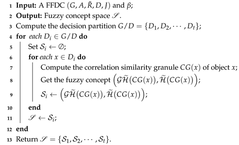
Definition 2.

Given a fuzzy formal context $(G,A,\tilde{R})$, for any $x_i,x_j\in G$, the correlation coefficient between $x_i$ and $x_j$ is defined as follows:

$$\begin{array}{c}\hfill r(x_i,x_j)={\displaystyle \frac{{\displaystyle \sum _{k=1}^m} |\tilde{R}(i,k)-\overline{R}\left(i\right)\left|\right|\tilde{R}(j,k)-\overline{R}\left(j\right)|}{\sqrt{{\displaystyle \sum _{k=1}^m}{(\tilde{R}(i,k)-\overline{R}\left(i\right))}^2}\sqrt{{\displaystyle \sum _{k=1}^m}{(\tilde{R}(j,k)-\overline{R}\left(j\right))}^2}}},\end{array}$$

(2)

where $\tilde{R}(i,k)$ denotes the membership degree of object $x_i$ with respect to attribute $a_k$, while $\overline{R}\left(i\right)$ represents the average membership degree of $x_i$ across the attribute set A. That is to say, $\overline{R}\left(i\right)={\displaystyle \frac{1}{m}}{\displaystyle \sum _{i=1}^m}\tilde{R}(i,k)$. The value of $r(x_i,x_j)$ explains the similarity degree between $x_i$ and $x_j$. The pairwise correlation coefficients form a symmetric matrix Q, where $Q(i,j)=r(x_i,x_j)$ quantifies the linear relationship between objects $x_i$ and $x_j$. Meanwhile, this correlation coefficient matrix can be used to construct the correlation similarity granule.

Definition 3.

Given an FFDC $(G,A,\tilde{R},D,J)$, for any $D_i\in G/D$, the correlation similarity granule of object x is given by

$$CG\left(x\right)=\{y\in D_i|r(x,y)\ge \beta \},$$

(3)

where β is a threshold and $CG\left(x\right)$ is the correlation similarity degree between x and y.

Definition 4.

Given an FFDC $(G,A,\tilde{R},D,J)$, where $G/D=\{D_1,D_2,\cdots ,D_t\}$, for any $D_i$, the fuzzy concept subspace ${𝒮}_i$ about $D_i$ is denoted as follows:

$${𝒮}_i=\left\{\left(\mathcal{G}\tilde{\mathcal{H}}\left(CG\left(x\right)\right),\tilde{\mathcal{H}}\left(CG\left(x\right)\right)\right)|x\in D_i\right\}.$$

(4)

where β is a threshold and $CG\left(x\right)$ is the correlation similarity degree between x and y.

Subsequently, we denote by $\mathcal{S}=\{{𝒮}_1,{𝒮}_2,\cdots ,{𝒮}_t\}$ the fuzzy concept space, where ${𝒮}_i$ is named a fuzzy subspace of $\mathcal{S}$. It should be emphasized that comprehensive feature learning of each individual object serves as a prerequisite for achieving optimal classification performance. Then we propose the procedure of constructing the fuzzy concept space in Algorithm 1 with the time complexity of $O\left(\right|G{|}^2\left|A\right|)$.

Algorithm 1: Constructing fuzzy concept space (CFCS).

Example 1.

Table 1 is an FFDC $(G,A,\tilde{R},D,J)$, where $G=\{x_1,x_2,x_3,x_4,x_5,x_6,x_7,x_8\}$ and $A=\{a_1,a_2,a_3,a_4\}$. d is the decision attribute that partitions all objects into two classes, with $D_1=\{x_1,x_2,x_3,x_4\}$ and $D_2=\{x_5,x_6,x_7,x_8\}$. The correlation coefficient matrix Q is computed as follows:

$$Q=\left[\begin{array}{cccccccc}1.00& 0.87& 0.74& 0.83& 0.48& 0.83& 0.98& 0.87\\ 0.87& 1.00& 0.95& 0.72& 0.67& 0.79& 0.90& 0.94\\ 0.74& 0.95& 1.00& 0.54& 0.70& 0.83& 0.76& 0.96\\ 0.83& 0.72& 0.54& 1.00& 0.69& 0.65& 0.90& 0.59\\ 0.48& 0.67& 0.70& 0.69& 1.00& 0.65& 0.90& 0.59\\ 0.83& 0.79& 0.83& 0.65& 0.68& 1.00& 0.80& 0.92\\ 0.98& 0.90& 0.76& 0.90& 0.59& 0.80& 1.00& 0.84\\ 0.87& 0.94& 0.96& 0.59& 0.60& 0.92& 0.84& 1.00\end{array}\right].$$

Given $\beta =0.65$, for the objects in decision class $D_1$, we can have the correlation similarity granule $CG\left(x_1\right)=\{x_1,x_2,x_3,x_4\}$, $CG\left(x_2\right)=\{x_1,x_2,x_3,x_4\}$, $CG\left(x_3\right)=\{x_1,x_2,x_3\}$, and $CG\left(x_4\right)=\{x_1,x_2,x_4\}$. Next, fuzzy concept subspace ${𝒮}_1=\{(\{x_1,x_2,x_3,x_4\},(0.1,0.3,0.4,0.4)),(\{x_1,x_2,x_3\},$$(0.1,0.3,0.4,0.5)\left)\right\}$.

For the objects in decision class $D_2$, their correlation similarity granule and fuzzy concept subspace are as follows: $CG\left(x_5\right)=\{x_5,x_6\},CG\left(x_6\right)=\{x_5,x_6,x_7,x_8\}$, $CG\left(x_7\right)=\{x_6,x_7,x_8\}$ and $CG\left(x_8\right)=\{x_6,x_7,x_8\}$. ${𝒮}_2=\{(\{x_5,x_6\},(0.3,0.4,0.3,0.4)),(\{x_5,x_6,x_7,x_8\},(0.1,0.4,0.3,0.3)),$$(\{x_6,x_7,x_8\},(0.1,0.5,0.4,0.3))\}$.

Table 1. An FFDC.

U	a1	a2	a3	a4	d
$x_1$	0.7	0.3	0.4	0.5	1
$x_2$	0.1	0.8	0.5	0.9	1
$x_3$	0.3	0.5	0.6	0.7	1
$x_4$	0.4	0.3	0.4	0.4	1
$x_5$	0.6	0.4	0.3	0.9	2
$x_6$	0.3	0.5	0.6	0.4	2
$x_7$	0.2	0.5	0.4	0.3	2
$x_8$	0.1	0.7	0.8	0.8	2

Table 1. An FFDC.

U	a1	a2	a3	a4	d
$x_1$	0.7	0.3	0.4	0.5	1
$x_2$	0.1	0.8	0.5	0.9	1
$x_3$	0.3	0.5	0.6	0.7	1
$x_4$	0.4	0.3	0.4	0.4	1
$x_5$	0.6	0.4	0.3	0.9	2
$x_6$	0.3	0.5	0.6	0.4	2
$x_7$	0.2	0.5	0.4	0.3	2
$x_8$	0.1	0.7	0.8	0.8	2

3.2. Constructing the Forgetting Fuzzy Concept Space

Section 3.1 discusses the construction process of the fuzzy concept space through the correlation similarity granule and a pair of cognitive operators $\tilde{\mathcal{H}}$ and $\mathcal{G}$. However, since $X\subseteq \mathcal{G}\tilde{\mathcal{H}}\left(X\right)$, some of the objects in extent $\mathcal{G}\tilde{\mathcal{H}}\left(X\right)$ may be forgotten because of knowledge forgetting.

Definition 5.

Given an FFDC $(G,A,\tilde{R},D,J)$, for arbitrary $X\subseteq G$, the inner fringe of X is denoted as

$$\hslash \left(X\right)=\left\{\mathcal{G}\tilde{\mathcal{H}}\left(X\right)\setminus Y_i|Y_j⊈Y_i, for any Y_j\in \Psi (i\ne j)\right\}.$$

(5)

where $\Psi =\left\{L(\tilde{\mathcal{H}}(X),a)|a\in A,\tilde{\mathcal{H}}\left(X\right)\left(a\right)\ne 0\right\}=\left\{Y_1,Y_2,\cdots Y_{|\Psi |}\right\}$ and $L(\tilde{\mathcal{H}}(X),a)=\left\{g\in \mathcal{G}\tilde{\mathcal{H}}\left(X\right)|\tilde{R}(g,a)=\tilde{\mathcal{H}}\left(X\right)\left(a\right)\right\}$ for $a\in A$.

Definition 5 introduces a method for forgetting the minimal object set that is proximate to a certain object in the extent $\mathcal{G}\tilde{\mathcal{H}}\left(X\right)$. Then the above forgetting minimal object set can be represented by a Boolean matrix, shown as Proposition 1.

Proposition 1.

Let $(G,A,\tilde{R},D,J)$ be an FFDC. $\hslash \left(X\right)$ is an inner fringe of $X\subseteq G$. Then, we know the following:

$$\hslash \left(X\right)=\left\{\mathcal{G}\tilde{\mathcal{H}}\left(X\right)\setminus Y_i|\sum _{j=1}^{|\Psi |}{d}_{ij}=1,Y_i\in \Psi \right\}.$$

(6)

where $\Psi =\left\{L(\tilde{\mathcal{H}}(X),a)|a\in A,\tilde{\mathcal{H}}(X)(a)\ne 0\right\}=\left\{Y_1,Y_2,\cdots Y_{|\Psi |}\right\}$ and

$$d_{ij}=\left\{\begin{array}{cc}\hfill 1,& Y_j\subseteq Y_i,\\ \hfill 0,& otherwise.\end{array}\right.$$

for $i,j=1,2,\cdots ,|\hslash |$.

Proof. 

For any $Y_i\in \Psi$, ${\sum }_{j=1}^{|\hslash |}{d}_{ij}=1$ means that

$$d_{ij}=\left\{\begin{array}{cc}\hfill 1,& j=i,\\ \hfill 0,& j\ne i.\end{array}\right.$$

That is to say, for any any $Y_j\in \Psi (j\ne i)$, it implies that $Y_j⊈Y_i$. Hence, for any $Y_i\in \Psi$, if ${\sum }_{j=1}^{|\hslash |}{d}_{ij}=1$, then it is obvious that $\mathcal{G}\tilde{\mathcal{H}}\left(X\right)\setminus Y_i\in \hslash \left(X\right)$.   □

Proposition 2.

Let $(G,A,\tilde{R},D,J)$ be an FFDC. $\hslash \left(X\right)$ is an inner fringe of $X\subseteq G$. For any $V_i\in \hslash \left(X\right)$, $\left(\mathcal{G}\tilde{\mathcal{H}}\left(V_i\right),\tilde{\mathcal{H}}\left(V_i\right)\right)$ is a fuzzy concept.

Proof. 

It is obvious from Definition 1.   □

In fact, there are multiple elements in $\hslash \left(X\right)$. After applying knowledge forgetting, the obtained forgetting fuzzy concept $(\mathcal{G}\tilde{\mathcal{H}}\left(V_i\right),\tilde{\mathcal{H}}\left(V_i\right))$ is defined, which is maximally similar to fuzzy concept $(\mathcal{G}\tilde{\mathcal{H}}\left(X\right),\tilde{\mathcal{H}}\left(X\right))$. For two concepts $(\mathcal{G}\tilde{\mathcal{H}}\left(V_i\right),\tilde{\mathcal{H}}\left(V_i\right))$ and $(\mathcal{G}\tilde{\mathcal{H}}\left(X\right),\tilde{\mathcal{H}}\left(X\right))$, the similarity degree is $K\left((\mathcal{G}\tilde{\mathcal{H}}\left(V_i\right),\tilde{\mathcal{H}}\left(V_i\right)),(\mathcal{G}\tilde{\mathcal{H}}\left(X\right),\tilde{\mathcal{H}}\left(X\right))\right)={\displaystyle \frac{|\mathcal{G}\tilde{\mathcal{H}}\left(V_i\right)\cap \mathcal{G}\tilde{\mathcal{H}}\left(X\right)|}{|\mathcal{G}\tilde{\mathcal{H}}\left(V_i\right)\cup \mathcal{G}\tilde{\mathcal{H}}\left(X\right)|}}+\sqrt{{\sum }_{a\in A}{(\tilde{\mathcal{H}}\left(V_i\right)-\tilde{\mathcal{H}}\left(X_i\right))}^2}$.

Definition 6.

Let $(G,A,\tilde{R},D,J)$ be an FFDC. For $(\mathcal{G}\tilde{\mathcal{H}}\left(X\right),\tilde{\mathcal{H}}\left(X\right))\in {\mathcal{S}}_i$, the collection of forgetting fuzzy concepts is defined as follows:

$${\mathcal{F}}_X^i=\left\{(\mathcal{G}\tilde{\mathcal{H}}\left(V_i\right),\tilde{\mathcal{H}}\left(V_i\right))|K\left((\mathcal{G}\tilde{\mathcal{H}}\left(V_i\right),\tilde{\mathcal{H}}\left(V_i\right)),(\mathcal{G}\tilde{\mathcal{H}}\left(X\right),\tilde{\mathcal{H}}(X))\right)=Max0 for V_i\in \hslash \left(X\right)\right\},$$

(7)

where $Max0=ma{x}_{V_i\in \hslash \left(X\right)}K\left((\mathcal{G}\tilde{\mathcal{H}}\left(V_i\right),\tilde{\mathcal{H}}\left(V_i\right)),(\mathcal{G}\tilde{\mathcal{H}}\left(X\right),\tilde{\mathcal{H}}\left(X\right))\right)$.

In a fuzzy formal decision context $(G,A,\tilde{R},D,J)$ and $X\subseteq G$, there are some fuzzy subconcepts of $(\mathcal{G}\tilde{\mathcal{H}}\left(X\right),\tilde{\mathcal{H}}\left(X\right))$; that is, certain fuzzy concepts can be obtained from $(\mathcal{G}\tilde{\mathcal{H}}\left(X\right),\tilde{\mathcal{H}}\left(X\right))$ after knowledge forgetting through the inner fringe $\hslash \left(X\right)$. From Proposition 2, for any $V_i\in \hslash \left(X\right)$, $(\mathcal{G}\tilde{\mathcal{H}}\left(V_i\right),\tilde{\mathcal{H}}\left(V_i\right))$ is a fuzzy concept obtained from $(\mathcal{G}\tilde{\mathcal{H}}\left(X\right),\tilde{\mathcal{H}}\left(X\right))$ after knowledge forgetting. It is obvious that $(\mathcal{G}\tilde{\mathcal{H}}\left(V_i\right),\tilde{\mathcal{H}}\left(V_i\right))\le (\mathcal{G}\tilde{\mathcal{H}}\left(X\right),\tilde{\mathcal{H}}\left(X\right))$. The higher the similarity between $(\mathcal{G}\tilde{\mathcal{H}}\left(V_i\right),\tilde{\mathcal{H}}\left(V_i\right))$ and $(\mathcal{G}\tilde{\mathcal{H}}\left(X\right),\tilde{\mathcal{H}}\left(X\right))$, the higher the probability that objects in $\mathcal{G}\tilde{\mathcal{H}}\left(X\right)\setminus Y_i$ are forgotten.

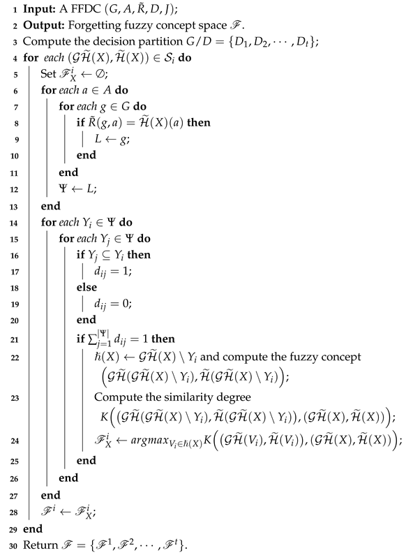
In addition, given $D_i$, the forgetting fuzzy concept subspace is denoted as ${\mathcal{F}}^i=\left\{{\mathcal{F}}_X^i|(\mathcal{G}\tilde{\mathcal{H}}\left(X\right),\tilde{\mathcal{H}}\left(X\right))\in {𝒮}_i\right\}$. At the same time, the process of constructing the forgetting fuzzy concept space is shown as Algorithm 2, where $\Psi$ is run in Steps 3–11, which can be taken in $O\left(\right|G{|}^2\left|A\right|)$, and some unnecessary objects are reduced in Steps 12–25, which can be measured in $O\left(\right|\Psi {|}^2\left|G\right|)$, where $\Psi$ means the zone of proximal development of an object. Hence, the time complexity of Algorithm 2 is ${O\left(\right|\mathcal{S}\left|\right(\left|G\right|}^2\left|A\right|+{|\Psi |}^2\left|G\right|\left)\right)$.

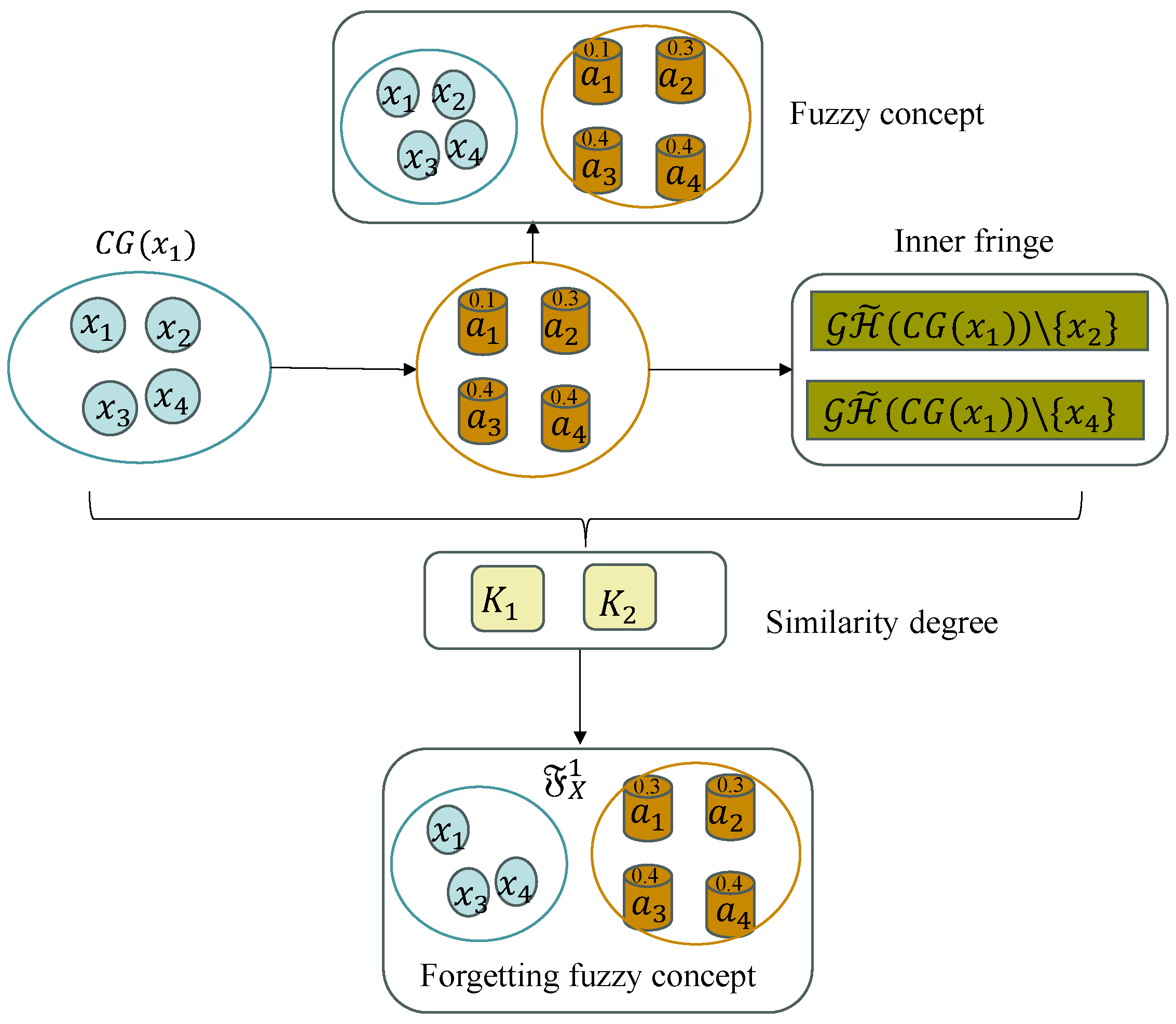
Example 2.

Continue with Example 1. With respect to class $D_1$, we now discuss the forgetting fuzzy concept of $(\{x_1,x_2,x_3,x_4\},(0.1,0.3,0.4,0.4))$ in ${𝒮}_1$. In fact, $\Psi =\{\left\{x_2\right\},\{x_1,x_4\},\left\{x_4\right\}\}$, which implies that $\hslash \left(X\right)=\{\{x_1,x_2,x_3,x_4\}\setminus \left\{x_2\right\},\{x_1,x_2,x_3,x_4\}\setminus \left\{x_4\right\}\}=\left\{\{x_1,x_3,x_4\},\{x_1,x_2,x_3\}\right\}$. Then we have two fuzzy concepts, $(\{x_1,x_3,x_4\},(0.3,0.3,0.4,0.4))$ and $(\{x_1,x_2,x_3\},(0.1,0.3,0.4,0.5))$. Subsequently, $K\left((\{x_1,x_3,x_4\},(0.3,0.3,0.4,0.4)),(\{x_1,x_2,x_3,x_4\},(0.1,0.3,0.4,0.4))\right)=0.95$ and $K\left((\{x_1,x_2,x_3\},(0.1,0.3,0.4,0.5)),(\{x_1,x_2,x_3,x_4\},(0.1,0.3,0.4,0.4))\right)=0.85$. Hence, we know that ${\mathcal{F}}_X^1=\left\{(\{x_1,x_3,x_4\},(0.3,0.3,0.4,0.4))\right\}$. Similarly, ${\mathcal{F}}_Y^1=\left\{(\{x_2,x_3\},(0.1,0.5,0.5,0.7))\right\}$. Finally, we have the forgetting fuzzy concept subspace ${\mathcal{F}}^1=\{(\{x_1,x_3,x_4\},(0.3,0.3,0.4,0.4)),(\{x_2,x_3\},$$(0.1,0.5,0.5,0.7)\left)\right\}$.

In addition, the forgetting fuzzy concept subspace in $D_2$ is ${\mathcal{F}}^2=\{(\left\{x_5\right\},(0.6,0.4,0.3,0.9)),$$(\{x_6,x_7,x_8\},(0.1,0.5,0.4,0.3)),(\{x_6,x_8\},(0.1,0.5,0.6,0.4))\}$.

Meanwhile, the process of learning the forgetting fuzzy concept is shown in Figure 2.

Algorithm 2: Constructing forgetting fuzzy concept space (CFFCS).

3.3. Fusing Concept

Mutual information exists among forgetting fuzzy concepts, manifested through their bidirectional influence mechanisms. In order to overcome the limitations of individual cognition and the incomplete cognitive environment [28], we propose a new method to fuse concepts through the forgetting fuzzy concept space.

Definition 7.

Given an FFDC $(G,A,\tilde{R},D,J)$, for a forgetting fuzzy concept subspace ${\mathcal{F}}^i$, if there exist forgetting fuzzy concepts $(X_1,{\tilde{B}}_1)$, $(X_2,{\tilde{B}}_2),\cdots ,(X_n,{\tilde{B}}_n)$ satisfying $X_1\subseteq X_2\subseteq \cdots \subseteq X_n$, then $(X_n,{\tilde{B}}_n)$ is regarded as the supremum fuzzy concept, and then the fusing forgetting fuzzy pseudo-concept $({\mathbf{Y}}_{i,j},{\tilde{\mathbf{B}}}_{i,j})$ is defined as follows:

$$\begin{array}{c}{\mathbf{Y}}_{i,j}=X_1\cup X_2\cup \cdots \cup X_n,\hfill \\ {\tilde{\mathbf{B}}}_{i,j}={\displaystyle \frac{1}{2^{n-1}}}({\tilde{B}}_1+{\tilde{B}}_2+2{\tilde{B}}_3+4{\tilde{B}}_4+\cdots +2^{n-1}{\tilde{B}}_n).\hfill \end{array}$$

(8)

where n means the number of forgetting fuzzy concepts.

Generally speaking, the fusing forgetting fuzzy concept space is denoted as $\mathcal{K}=\{{\mathcal{K}}_1,{\mathcal{K}}_2,\cdots ,{\mathcal{K}}_t\}$, where ${\mathcal{K}}_i=\left\{{\mathcal{K}}_{i,j}\right|j=1,2,\cdots ,n\}=\left\{({\mathbf{Y}}_{i,j},{\tilde{\mathbf{B}}}_{i,j})\right|j=1,2,\cdots ,n\}$, in which n is the number of pseudo-concepts in ${\mathcal{K}}_i$. The intent ${\tilde{\mathbf{B}}}_{i,j}$ explicitly characterizes the magnitude of the pseudo-concept, in which the intents of subconcepts have been assigned different weights according to their corresponding extents. In other words, the greater the extent $X_i$ is, the larger the weight of its corresponding intent ${\tilde{B}}_i$ is. Finally, Algorithm 3 describes the clustering process of the fusing forgetting fuzzy concept space with the worst-case time complexity of $O\left(\right|G{|}^2\left|A\right|)$.

Algorithm 3: Cognitive process of fusing forgetting fuzzy concept space.

Example 3.

Continuing to Example 2, according to Definition 7, fusing forgetting fuzzy concept spaces are represented as follows:

$$\begin{array}{c}{\mathcal{K}}_{1,1}=(\{x_1,x_3,x_4\},(0.3,0.3,0.4,0.4));\hfill \\ {\mathcal{K}}_{1,2}=(\{x_2,x_3\},(0.1,0.5,0.5,0.7));\hfill \\ {\mathcal{K}}_{2,1}=(\left\{x_5\right\},(0.6,0.4,0.3,0.9));\hfill \\ {\mathcal{K}}_{2,2}=(\{x_6,x_7,x_8\},(0.1,0.5,0.5,0.35)).\hfill \end{array}$$

(9)

It should be noted that there are two fusing forgetting fuzzy concepts in each decision class. It is evident that these concepts preserve the initial information while eliminating the redundant forgetting fuzzy concepts, which significantly enhances the efficiency of concept-cognitive learning.

3.4. Class Prediction

It should be noted that the class prediction of a testing sample is primarily determined based on the Euclidean distance between the testing sample and existing fuzzy concept clustering space [27,29,30].

Definition 8.

Let $x_{new}$ be a testing sample. $(x_{new},\tilde{\mathcal{H}}\left(x_{new}\right))$ is a new fuzzy concept; then the distance between $\tilde{\mathcal{H}}(x_{new})$ and pseudo-concept $({\mathbf{Y}}_{i,j},{\tilde{\mathbf{B}}}_{i,j})$ in ${\mathcal{K}}_i$ is defined as follows:

$$\begin{array}{c}\hfill \begin{array}{c}\hfill Dis(\tilde{\mathcal{H}}\left(x_{new}\right),{\tilde{\mathbf{B}}}_{i,j})=\sqrt{\sum _{a\in A}{(\tilde{\mathcal{H}}\left(x_{new}\right)\left(a\right)-{\tilde{\mathbf{B}}}_{i,j}\left(a\right))}^2}.\end{array}\end{array}$$

(10)

As is well known, $Dis(\tilde{\mathcal{H}}\left(x_{new}\right),{\tilde{\mathbf{B}}}_{i,j})$ is the distance similarity. The smaller the distance value $Dis(\tilde{\mathcal{H}}\left(x_{new}\right),{\tilde{\mathbf{B}}}_{i,j})$, the stronger the correlation between two fuzzy concepts. Consequently, class determination for a new sample can be achieved by computing their similarity. Algorithm 4 describes the class prediction with the time complexity of $O\left(\right|\mathcal{K}\left|\right|A\left|\right)$.

Algorithm 4: Class prediction of testing sample.

Example 4.

In the FFDC of Table 2, where $x_1-x_8$ are from Example 1, $x_9-x_{10}$ are two new testing objects.

Regarding the object $x_9$, the membership degree about $\tilde{R}$ is $\tilde{\mathcal{H}}\left(x_{new}\right)=(0.6,0.5,0.1,0.6)$, while its true label is 2. Subsequently, the Euclidean distance between $x_9$ and the existing fusing forgetting fuzzy concept space $\mathcal{K}$ is computed as follows: $Dis(\tilde{\mathcal{H}}\left(x_{new}\right),{\tilde{\mathbf{B}}}_{1,1})=0.5099$, $Dis(\tilde{\mathcal{H}}\left(x_{new}\right),{\tilde{\mathbf{B}}}_{1,2})=0.6481$, $Dis(\tilde{\mathcal{H}}\left(x_{new}\right),{\tilde{\mathbf{B}}}_{2,1})=0.3742$, and $Dis(\tilde{\mathcal{H}}\left(x_{new}\right),{\tilde{\mathbf{B}}}_{2,2})=0.6874$. Indeed, the distance between $\tilde{\mathcal{H}}\left(x_{new}\right)$ and ${\tilde{\mathbf{B}}}_{2,1}$ attains its minimum in ${\mathcal{K}}_2$. Consequently, $x_9$ should be classified into decision class $D_2$, which perfectly matches its real label 2.

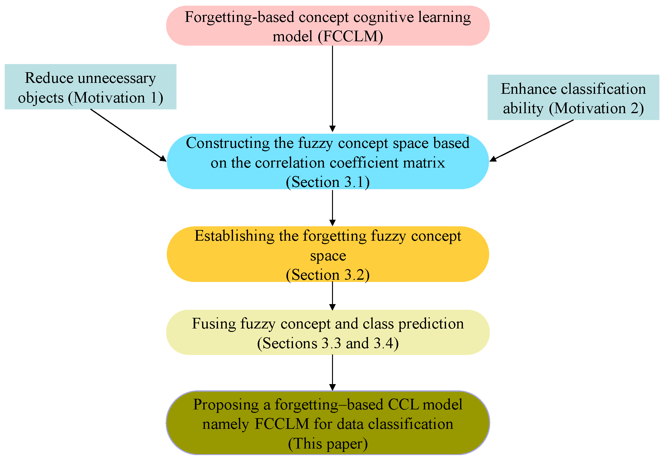
Based on the above discussion, Figure 3 describes the overall flowchart of the FCCLM, which includes four parts, namely (1) constructing a fuzzy concept space; (2) constructing a forgetting fuzzy concept space; (3) constructing a fusing forgetting fuzzy concept space; and (4) class prediction. In summary, the total time complexity of our model FCCLM is ${O\left(max\right\{\left|\mathcal{S}\right|\left(\right|G|}^2\left|A\right|+{|\Psi |}^2\left|G\right|),|\mathcal{K}\left|\right|A\left|\right\})$.

Table 2. A FFDC.

U	a1	a2	a3	a4	d
$x_1$	0.7	0.3	0.4	0.5	1
$x_2$	0.1	0.8	0.5	0.9	1
$x_3$	0.3	0.5	0.6	0.7	1
$x_4$	0.4	0.3	0.4	0.4	1
$x_5$	0.6	0.4	0.3	0.9	2
$x_6$	0.3	0.5	0.6	0.4	2
$x_7$	0.2	0.5	0.4	0.3	2
$x_8$	0.1	0.7	0.8	0.8	2
$x_9$	0.6	0.5	0.1	0.6	2
$x_{10}$	0.2	0.6	0.4	0.9	2

Table 2. A FFDC.

U	a1	a2	a3	a4	d
$x_1$	0.7	0.3	0.4	0.5	1
$x_2$	0.1	0.8	0.5	0.9	1
$x_3$	0.3	0.5	0.6	0.7	1
$x_4$	0.4	0.3	0.4	0.4	1
$x_5$	0.6	0.4	0.3	0.9	2
$x_6$	0.3	0.5	0.6	0.4	2
$x_7$	0.2	0.5	0.4	0.3	2
$x_8$	0.1	0.7	0.8	0.8	2
$x_9$	0.6	0.5	0.1	0.6	2
$x_{10}$	0.2	0.6	0.4	0.9	2

4. Experimental Results

To evaluate the classification efficacy of model FCCLM, a comparative analysis will be conducted between it and concept-cognitive learning as well as machine learning classification algorithms. A total of eight datasets are selected from the UCI (dataset source: http://archive.ics.uci.edu/, accessed on 14 March 2015) and Gene (Dataset source: https://jundongl.github.io/scikit-feature/datasets.html, accessed on 14 March 2015) data set repositories, as detailed in

Table 3. Data description.

ID	Dataset	Object	Attribute	Class
1	Appendicitis	106	7	2
2	Dermatology	358	34	6
3	Movement	360	90	15
4	Air	359	64	3
5	Austra	690	14	2
6	Sonar	208	60	2
7	Wdbc	569	30	2
8	Wine	178	13	3

.

4.1. Experimental Setting

As a preprocessing step, Max–Min normalization is applied to all attributes to guarantee dataset compatibility with fuzzy processing requirements, specifically given by

$$\begin{array}{c}\hfill \tilde{R}(u_i,a_j)={\displaystyle \frac{f(u_i,a_j)-\min \left(f\left(a_j\right)\right)}{\max \left(f\left(a_j\right)\right)-\min \left(f\left(a_j\right)\right)}},\end{array}$$

where $f(u_i,a_j)$ is the initial value of object $u_i$ for attribute $a_j$. Additionally, $\max \left(f\left(a_j\right)\right)$ and $\min \left(f\left(a_j\right)\right)$ are the maximum and minimum values of attribute $a_j$ across all objects, respectively.

In the experiment, we compare FCCLM with three concept-cognitive learning classification algorithms, namely, DMPWFC [23], ILMPFTC [24], and FCLM [21]. Furthermore, we also compare FCCLM with four machine learning classification algorithms, including Complex Tree (CT), Fuzzy-Root-Sum-Square (F-RSS), Decision Tree (DT), and Fuzzy Classification and Regression Tree (F-CART). Notice that parameter $\beta$ plays an important role in constructing correlation similarity granules. In this investigation, parameter $\beta$ is varied systematically from 0.55 to 1.0 with a step size of 0.05 to influence correlation similarity granules. All analyses are conducted using five-fold cross-validation to guarantee unbiased performance estimation. Final performance metrics are computed as the mean values obtained from the five cross-validation test partitions. All results are generated in MATLAB 2021a using standardized hardware (Intel(R) Core(TM) i7-4790 CPU @ 3.6 GHz, 16 GB (Lenovo, Quanzhou, China)) to ensure computational consistency.

4.2. Results and Analyses

The results of accuracy and the optimal parameter $\beta$ of the proposed algorithm FCCLM and seven classification algorithms on eight datasets are shown in

Table 4. Accuracy comparison (mean ± standard deviation%) of FCCLM and seven other algorithms.

ID	β	FCCLM	DMPWFC	ILMPFTC	FCLM	CT	F-RSS	DT	F-CART
1	0.80	86.75 ± 5.29	73.14 ± 12.03	57.80 ± 23.06	63.76 ± 19.02	83.89 ± 5.56	86.70 ± 8.85	74.50 ± 2.84	83.89 ± 4.43
2	0.95	96.36 ± 1.16	95.16 ± 2.29	95.92 ± 2.68	40.52 ± 3.00	94.68 ± 2.31	53.93 ± 10.06	61.77 ± 7.97	94.13 ± 2.09
3	1.00	81.67 ± 3.85	82.76 ± 4.86	87.29 ± 5.08	66.69 ± 3.23	61.67 ± 5.07	38.33 ± 4.77	14.44 ± 5.07	57.70 ± 11.31
4	1.00	95.83 ± 3.11	95.56 ± 1.95	82.61 ± 4.80	54.49 ± 5.80	85.52 ± 3.59	45.41 ± 7.73	50.09 ± 10.52	80.50 ± 3.83
5	1.00	80.14 ± 3.53	84.53 ± 3.32	53.05 ± 3.97	65.23 ± 4.54	84.78 ± 3.12	78.99 ± 1.85	72.46 ± 6.62	84.20 ± 4.45
6	1.00	86.09 ± 7.80	60.89 ± 14.58	82.57 ± 7.54	66.79 ± 12.77	71.18 ± 12.17	68.78 ± 4.86	65.82 ± 10.01	72.13 ± 10.35
7	1.00	93.32 ± 1.01	41.71 ± 16.69	83.07 ± 3.70	70.65 ± 1.15	78.09 ± 1.47	77.72 ± 0.90	88.93 ± 4.09	92.79 ± 1.34
8	0.95	96.63 ± 1.23	27.16 ± 37.90	89.05 ± 6.40	68.87 ± 26.22	92.67 ± 5.83	93.84 ± 2.29	66.81 ± 7.83	89.35 ± 6.61
Ave. ± SD		89.60 ± 3.37	70.11 ± 11.70	78.92 ± 7.15	62.13 ± 9.47	81.56 ± 4.89	67.96 ± 5.16	61.85 ± 6.87	81.84 ± 5.55
Rank		1.63	4.88	4.25	6.38	3.56	5.25	6.13	3.94
Win/tie/loss		6/0/8	0/0/8	1/0/8	0/0/8	1/0/8	0/0/8	0/0/8	0/0/8

. The bottom row displays the mean classification accuracy with the standard deviation, where bold–underline formatting highlights the algorithm’s statistically superior performance compared to all baseline methods. The results of the table indicate that ILMPFTC and CT achieve optimal accuracy on one dataset, respectively, while FCCLM demonstrates superior performance across six datasets. Furthermore, FCCLM has a higher average accuracy and lower standard deviation than the other algorithms, which indicates that the performance of FCCLM outperforms the other seven algorithms. The average accuracy of FCCLM is increased by 9.48% when compared to F-CART on all selected datasets. In summary, the above results indicate that FCCLM is superior to the other models. Figure 4 depicts the accuracy comparison between CCL and the other seven algorithms. This figure describes the accuracy of FCCLM, which possesses a smaller fluctuation range than the other algorithms in most datasets.

Subsequently, the results of recall for the proposed algorithm FCCLM and seven classification algorithms on eight datasets are presented in

Table 5. Recall comparison (mean ± standard deviation%) of FCCLM and seven other algorithms.

ID	β	FCCLM	DMPWFC	ILMPFTC	FCLM	CT	F-RSS	DT	F-CART
1	0.80	75.36 ± 11.83	74.71 ± 24.04	57.13 ± 26.77	63.33 ± 27.71	65.21 ± 9.71	71.00 ± 19.64	67.02 ± 8.87	68.96 ± 8.78
2	0.95	95.83 ± 2.08	92.58 ± 11.35	95.41 ± 9.56	27.72 ± 35.27	94.03 ± 2.81	36.76 ± 3.98	-	92.42 ± 1.92
3	1.00	80.43 ± 4.79	58.54 ± 39.32	84.29 ± 22.15	68.69 ± 18.01	62.05 ± 5.15	44.73 ± 2.23	-	67.70 ± 16.54
4	1.00	95.54 ± 3.46	95.29 ± 7.05	80.90 ± 10.11	56.12 ± 30.88	85.35 ± 3.75	38.65 ± 3.28	-	80.23 ± 4.47
5	1.00	79.62 ± 4.02	83.85 ± 3.32	54.40 ± 14.09	64.76 ± 18.61	84.75 ± 3.35	76.89 ± 1.06	62.36 ± 13.42	83.92 ± 3.94
6	1.00	85.86 ± 7.84	-	87.86 ± 6.04	77.77 ± 17.59	71.60 ± 13.00	66.81 ± 4.94	-	71.77 ± 10.35
7	1.00	90.90 ± 2.26	-	84.82 ± 10.02	76.85 ± 31.02	91.92 ± 2.80	82.58 ± 3.28	-	92.58 ± 1.37
8	0.95	97.19 ± 0.94	-	90.33 ± 11.09	33.33 ± 57.74	93.20 ± 5.42	93.95 ± 1.70	56.37 ± 14.56	88.28 ± 7.52
Ave. ± SD		87.59 ± 4.65	80.99 ± 17.01	79.39 ± 13.73	58.57 ± 29.60	81.01 ± 5.75	63.92 ± 5.01	61.91 ± 12.28	80.73 ± 6.86

. The last row illustrates the average accuracy and standard deviation, with bold–underline formatting denoting statistically superior performance relative to comparator algorithms. This table indicates that ILMPFTC, CT, and F-CART achieve the best accuracy twice, once, and once, respectively, while FCCLM has the best performance on four datasets. Furthermore, FCCLM demonstrates statistically superior performance, exhibiting both a significantly higher average accuracy and lower standard deviation compared to the other algorithms, which illustrates that the performance of FCCLM outperforms the other seven algorithms.

Figure 5 describes the classification accuracy as $\beta$ changes. From this figure, we can observe that the accuracy shows a slow upward trend with fluctuations as the parameter varies, among which the fluctuation range is the largest in the interval [0.75, 0.85]. At the same time, most datasets achieve optimal accuracy in the range of [0.85, 0.95].

Additionally, the statistical significance of the eight classification algorithms could be compared using the Friedman test [31] and Bonferoni–Dunn test [32]. For the Friedman test, a Fisher distribution $F_F$ measuring the performance of different algorithms is given by

$$F_F={\displaystyle \frac{(N-1){\chi }_F^2}{N(k-1)-{\chi }_F^2}}\sim F\left(k-1,k-1(N-1)\right)$$

(11)

where ${\chi }_F^2={\displaystyle \frac{12N}{k(k+1)}}({\sum }_{i=1}^k{R}_i^2-{\displaystyle \frac{k{(k+1)}^2}{4}})$. N is the number of datasets, k is the cardinality of different algorithms, and $R_i$ is the average rank of algorithm $R_i$ across all datasets. We first assume the null hypothesis that no statistically significant differences exist in predictive accuracy among the compared classification methods. If $F_F>F\left(k-1,k-1(N-1)\right)$, then the initial hypothesis will be rejected. The rank result of the eight models is represented in

Table 6. Rank of classification algorithms.

ID	FCCLM	DMPWFC	ILMPFTC	FCLM	CT	F-RSS	DT	F-CART
1	1	6	8	7	3.5	2	5	3.5
2	1	3	2	8	4	7	6	5
3	3	2	1	4	5	7	8	6
4	1	2	4	6	3	8	7	5
5	4	2	8	7	1	5	6	3
6	1	8	2	6	4	5	7	3
7	1	8	4	7	5	6	3	2
8	1	8	5	6	3	2	7	4
Average	1.63	4.88	4.25	6.38	3.56	5.25	6.13	3.94

. In fact, $F_F=4.5634$, and the critical value of $F(7,49)=2.203$ at level $\alpha =0.05$. Therefore, we reject the null hypothesis and accept the alternative hypothesis that the classification performance of the eight models is remarkably different.

Subsequently, the Bonferroni–Dunn test is applied to conduct pairwise comparisons of classification performance among the five top-performing models. Assume that the mean rank between two models exceeds the critical value

$$C{D}_{\alpha }=q_{\alpha }\sqrt{{\displaystyle \frac{k(k+1)}{6N}}}$$

and then the above two models exhibit statistically significant differences in classification performance, in which $q_{\alpha }$ is denoted as the critical value in the test.

At level $\alpha =0.05$, we notice that the critical value $q_{0.05}=2.690$ in [32]. Subsequently, $C{D}_{\alpha }=3.2946$ ($k=8$ and $N=8$). Therefore, we can see from Figure 6 that algorithm FCCLM outperforms algorithms F-RSS, FCLM, and DT at level $\alpha =0.05$.

4.3. Discussion

In the above subsection, we compare the performance of FCCLM with other algorithms using eight datasets. Experimental results demonstrate the effectiveness and efficiency of our proposed algorithm FCCLM from the perspective of accuracy and statistical results. Specifically, some advantages are reflected on as follows: (1) We could counterpoise the sensitivity and specificity of Algorithm 1, named CFCS, to capture rich information by adjusting the threshold, thus facilitating the interpretability and understanding of the concept learning process. (2) Knowledge forgetting of the learned fuzzy concepts is performed through the inner fringe, thereby aligning with the logic of the Ebbinghaus forgetting curve and enhancing interpretability. (3) In the classification task, the fusing forgetting fuzzy pseudo-concept and class prediction can accelerate the acquisition of sample labels and reduce the time consumption of model FCCLM. In summary, a novel forgetting-based concept-cognitive learning model for classification in a fuzzy formal decision context is introduced to enhance the cognitive process.

5. Conclusions

In the context of rapidly expanding data, how to mine knowledge and fuse information is an important issue. Some existing CCL methods in the fuzzy formal decision context mainly focus on forgetting unnecessary concepts in constructing the concept space; ignoring the object is the key to constructing concepts. In this article, we have proposed a forgetting-based concept-cognitive learning model for classification tasks in a fuzzy formal decision context. Concretely, we firstly construct the fuzzy concept space with the correlation coefficient matrix. After that, in order to eliminate unnecessary objects in the zone of proximal development, we build a forgetting fuzzy concept space by choosing the concept with the highest similarity. Next, we propose a forgetting-based fuzzy concept model, which handles concept fusion and concept class prediction. Finally, to gain a better understanding of our proposed model, a series of comparative experiments on eight datasets are conducted to show that FCCLM can attain superior classification performance.

This article introduces a forgetting mechanism in the process of concept-cognitive learning, but does not consider recognition in the incremental learning process. Our future research will address this issue with the aim of enhancing the accuracy and efficiency of incremental learning approaches in the context of CCL.