A New Cluster Validity Index Based on Local Density of Data Points

Abstract

Multiple cluster validity indices (CVIs) have been introduced for diverse applications. In practice, clusters exhibit varying shapes, sizes, densities, and closely spaced centers, which are typically unknown beforehand. It is desirable to develop a versatile CVI that performs well in general settings rather than being tailored to specific ones. Drawing inspiration from distance based on local density, where it is observed that cluster centers feature higher densities than their neighbors and are relatively distant from higher-density points, this paper introduces a novel CVI. This CVI employs a modified distance, adjusted for local density, to measure cluster compactness, replacing the traditional Euclidean distance with the minimum distance to a higher-density point. This adjustment accounts for cluster shapes and densities. The experimental results highlight the proposed index’s dual capability: it not only outperforms conventional methods by a remarkable margin of 32 percentage points in controlled synthetic environments but also maintains a 23+ percentage-point accuracy lead in real-world data regimes characterized by noise and heterogeneity. This consistency validates its generalizability across data modalities.

1. Introduction

Clustering is a fundamental task in unsupervised learning, aiming to partition data points into homogeneous groups for exploratory analysis across diverse domains, including astronomy, bioinformatics, bibliometrics, and pattern recognition [1]. Despite the proliferation of clustering algorithms—categorized into center-based, density-based, hierarchical, and rational methods [2]—a persistent challenge lies in determining the optimal number of clusters (k) a priori. This challenge arises from the absence of a universally applicable definition for “natural clusters” in complex datasets, which often exhibit irregular shapes, varying densities, and overlapping structures [3].

Cluster validity indices (CVIs) serve as critical tools to address this challenge by quantifying the quality of clustering partitions. Traditional CVIs, such as the Dunn index [4], partition coefficient (PC) [5], Xie–Beni (XB) index [6], and their variants [7,8], typically rely on intra-cluster compactness and inter-cluster separation metrics derived from Euclidean distances. However, these indices often falter under realistic scenarios where clusters exhibit non-convex geometries, density variations, or closely spaced centers. For instance, indices like XB and PC assume spherical cluster shapes and uniform densities, leading to inaccurate k estimation when these assumptions are violated [9].

Recent advancements in CVIs have attempted to address these limitations. The WL index [9] incorporates median center distances to enhance separation measurement, while the I index [10] employs the Jeffrey divergence to account for cluster size and density. The CVM index [11] introduces core-based density estimation for handling complex structures. Nevertheless, challenges remain in robustly identifying clusters with arbitrary shapes, automatically excluding outliers, and maintaining stability across varying dimensionalities.

In this work, we propose the Relative Higher Density (RHD) index, inspired by the concept that cluster centers exhibit higher density than their neighbors while being distant from points of even higher density [1]. The RHD index measures compactness using the minimum distance to higher-density points, enabling it to: (1) identify clusters of arbitrary shapes and dimensionalities; (2) automatically detect and exclude outliers without preprocessing; (3) maintain stability in the presence of closely spaced centers.

We benchmark the RHD index against state-of-the-art CVIs (WL, I, and CVM) to demonstrate its superiority in handling complex clustering patterns, including non-convex geometries, partial overlap, and density variations.

2. Related Work

2.1. Clustering Algorithms and the Challenge of Determining k

Clustering algorithms play a pivotal role in data analysis, with applications spanning scientific and engineering disciplines [1]. Depending on their underlying models, they are broadly classified into center-based (e.g., k-means), density-based (e.g., DBSCAN), hierarchical (e.g., agglomerative clustering), and rational clustering methods [2]. Comprehensive reviews of these algorithms can be found in [12,13].

A critical challenge in clustering is specifying the optimal number of clusters (k). This task is non-trivial due to the lack of a universally accepted definition of clusters, which may vary in shape, density, and scale across datasets [3]. To address this, researchers have developed various methods, including statistical approaches (e.g., Bayesian information criterion [14]), resampling techniques (e.g., gap statistic [15]), and nonparametric methods [3,16]. Among these, CVIs are widely used to evaluate clustering quality by balancing compactness and separation criteria.

2.2. Cluster Validity Indices (CVIs)

CVIs quantify the goodness of clustering partitions by combining measures of intra-cluster cohesion and inter-cluster dispersion. Early CVIs, such as the Dunn index [4], introduced ratio-based metrics to balance compactness and separation. Bezdek’s PC and PE indices [5,17] focused on membership values to assess compactness, while the XB index [6] incorporated inter-center distances for separation. Subsequent variants, like the R index [7], refined these measures by including overlap metrics.

However, traditional CVIs often assume convex, equally sized clusters with uniform densities, limiting their effectiveness in real-world scenarios. For example, the XB index struggles with non-spherical clusters, and the Dunn index is sensitive to noise and outliers. To address these limitations, recent CVIs have introduced more sophisticated measures:

• WL index [9]: Considers both minimum and median center distances to improve separation assessment.
• I index [10]: Uses the Jeffrey divergence to account for cluster size and density variations.
• CVM index [11]: Focuses on core-based density estimation, making it robust to complex structures.

Despite these advancements, challenges persist in handling datasets with arbitrary cluster shapes, closely spaced centers, and outliers. The RHD index proposed in this work addresses these gaps by leveraging density-based distances to capture intrinsic cluster structures, as detailed in the following sections.

The remainder of this paper is organized as follows. In Section 2, some up-to-date CVIs commonly used in practice are briefly reviewed. In Section 3, the proposed RHD index is developed. In Section 4, some experimental studies based on the synthetic and real datasets are presented. Some concluding remarks are given in Section 5.

3. Traditional CVIs

Numerous CVIs have been proposed and extensively studied. For brevity, this section reviews only the up-to-date WL, I, and CVM indices for comparison with the proposed one. These indices represent significant improvements over earlier CVIs. To facilitate discussion, we define the notation as follows: $X=\{x_1,x_2,\dots ,x_n\}$ represents the dataset, where $x_i\in {\mathbb{R}}^d$ for $i=1,2,\dots ,n$, n is the total number of observations, and d is the dimension of observations; $C_j$ is the j-th cluster ($1\le j\le K$), K is the number of clusters, $v_j$ is the center of $C_j$; ${|·|}^2$ denotes the Euclidean distance; $u_{ij}$ denotes the membership degree of observation $x_i$ to cluster $C_j$. $S_j$ means the covariance matrix of the observations with cluster $C_j$. To maintain consistency with existing research, we set the fuzziness parameter $m=2$.

3.1. The WL Index

Wu et al. [9] noted that traditional CVIs often assume highly compact, weakly interlinked clusters—an unrealistic premise in practice. To overcome this, they introduced the WL index, which defines separation $S_{WL}\left(K\right)$ via two components, representing a departure from traditional definitions.

$$S_{WL}\left(K\right)={\displaystyle \frac{1}{2}}\left(\underset{i,j=1,\dots ,K;i\ne j}{min}\{|v_i-v_j{|}^2\}+\underset{i,j=1,\dots ,K;i\ne j}{\mathrm{median}}\{|v_i-v_j{|}^2\}\right).$$

(1)

In Equation (1), ${\displaystyle \underset{i,j=1,\dots ,K;i\ne j}{min}}\{|v_i-v_j{|}^2\}$ represents the minimum pairwise distance between cluster centers. The second component, ${\displaystyle \underset{i,j=1,\dots ,K;i\ne j}{\mathrm{median}}}\{|v_i-v_j{|}^2\}$, represents the median distance among all pairwise distances.

To define cluster compactness, the WL index incorporates both the membership value and the distance between an observation and its cluster center, defining it as:

$${\mu }_{ij}^2{|x_i-v_j|}^2,$$

(2)

where ${\mu }_{ij}$ is the membership value with ${\sum }_{j=1}^K{\mu }_{ij}=1$, which measures the probability of observation $x_i$ belonging to cluster $C_j$. The total compactness $C_{WL}\left(K\right)$ of all clusters can be expressed as:

$$C_{WL}\left(K\right)=\sum _{j=1}^K\left({\displaystyle \frac{{\mathsf{\Sigma }}_{i=1}^n{\mu }_{ij}^2{|x_i-v_j|}^2}{{\mathsf{\Sigma }}_{i=1}^n{\mu }_{ij}}}\right).$$

(3)

The WL index is defined as the ratio of the compactness measure to the new separation measure:

$$WL\left(K\right)={\displaystyle \frac{C_{WL}\left(K\right)}{S_{WL}\left(K\right)}}.$$

(4)

A good partition is characterized by high separation and low compactness. Thus, the optimal partition corresponds to the value of K that minimizes $WL\left(K\right)$.

3.2. The I Index

The I-index, proposed by Said et al. [10], resolves the issue of closely spaced cluster centers. Traditional Euclidean distance-based separation measures may fail to reflect the true separation, especially for clusters of varying sizes and densities. Consequently, Said et al. suggest the Jeffrey divergence as an alternative inter-cluster separation measure.

The Jeffrey divergence $JD(C_t,C_j)$ between clusters $C_t$ and $C_j$ is defined as:

$$\begin{array}{c}\hfill JD(C_t,C_j)={\displaystyle \frac{1}{2}}\left(\mathrm{tr}\left({\mathsf{\Sigma }}_t^{-1}{\mathsf{\Sigma }}_j\right)+\mathrm{tr}\left({\mathsf{\Sigma }}_j^{-1}{\mathsf{\Sigma }}_t\right)\right)\\ \hfill +{\displaystyle \frac{1}{2}}\left({(v_t-v_j)}^T({\mathsf{\Sigma }}_t^{-1}+{\mathsf{\Sigma }}_j^{-1})(v_t-v_j)\right)-d,\end{array}$$

(5)

where d is the dimension of the data, $v_j$ and ${\mathsf{\Sigma }}_j$ are the mean vector (i.e., cluster center) and covariance matrix of all the data observations in cluster $C_j$, respectively.

The new separation measure $S_I\left(K\right)$ is defined as:

$$S_I\left(K\right)=\sum _{j=1}^{K}Se{p}_j,$$

(6)

where

$$Se{p}_j=\underset{t,j=1,\dots ,K,j\ne t}{min}\left\{JD(C_t,C_j)\right\}.$$

(7)

The compactness measure $C_I\left(K\right)$ is computed as the summation of all clusters of the maximum distance of an observation to its center, given by:

$$C_I\left(K\right)=\sum _{j=1}^K\underset{x_i\in C_j}{max}\left\{|x_i-v_j{|}^2\right\}.$$

(8)

The I index is defined as the ratio of $S_I$ to $C_I$, namely,

$$I\left(K\right)={\displaystyle \frac{C_I\left(K\right)}{S_I\left(K\right)}}.$$

(9)

A small value of index I is an indicator of a good partition.

3.3. The CVM Index

The CVM index, proposed by Morsier et al. [11], is tailored for complex datasets with overlapping and differently shaped clusters and outliers. It focuses on the cluster core, a homogeneous group of similar samples representing the cluster’s natural variability. The CVM index includes three key terms: core size, core separability, and core homogeneity.

The core size $d_{\mathrm{in}}\left(C_j\right)$ is defined by the maximal distance observed among the samples in the cluster core:

$$d_{\mathrm{in}}\left(C_j\right)=\underset{x_i,x_s\in C_j}{max}\left\{|x_i-x_s{|}^2\right\}.$$

(10)

The core separability $d_{\mathrm{inter}}\left(C_j\right)$ is the minimum distance from a core sample in one cluster $C_l,l=1,2,\dots ,K$ to a core sample in another cluster $C_j,j=1,2,\dots ,K$, defined as:

$$d_{\mathrm{inter}}\left(C_j\right)=\underset{x_i\in C_l,x_t\in C_j,l\ne j}{min}\left\{|x_i-x_t{|}^2\right\}.$$

(11)

The distance $d_{\mathrm{inter}}\left(C_j\right)$ quantifies the smallest separation between cluster $C_j$ and any other cluster. The core homogeneity $R_{\mathrm{in}}\left(C_j\right)$ is the ratio of the maximum to the average smallest inner distances within the cluster core, defined as:

$$R_{\mathrm{in}}\left(C_j\right)={\displaystyle \frac{d_{{\max }_{\mathrm{i}}\mathrm{n}}\left(C_j\right)}{d_{{\mathrm{mean}}_{\mathrm{i}}\mathrm{n}}\left(C_j\right)}}={\displaystyle \frac{\underset{x_i\in C_j,i=1,\dots ,n_j}{\max }\left({\displaystyle \underset{x_s\in C_j,s\ne i}{min}}{|x_s-x_i|}^2\right)}{\frac{1}{|n_j|}\underset{x_i\in C_j,i=1,\dots ,n_j}{\mathsf{\Sigma }}\left({\displaystyle \underset{x_s\in C_j,s\ne i}{min}}{|x_s-x_i|}^2\right)}},$$

(12)

where $n_j$ is the number of observations in cluster $C_j$. Hence, the larger the ratio $R_{\mathrm{in}}\left(C_j\right)$, the more pronounced the heterogeneity of cluster $C_j$. A ratio close to 1 indicates a highly homogeneous core.

The CVM index is based on:

$$CVM\left(K\right)=\left(\sum _{j=1}^K{\displaystyle \frac{d_{\mathrm{in}}\left(C_j\right)}{R_{\mathrm{in}}\left(C_j\right)}}\right)·\left(\sum _{j=1}^K{d}_{\mathrm{inter}}\left(C_j\right)\right),$$

(13)

which maximizes the cluster core sizes $d_{\mathrm{in}}\left(j\right)$ rescaled by $1/R_{\mathrm{in}}\left(j\right)$ and the cluster cores separability. A large value of index CVM indicates a good partition. The CVM would be small when the cluster cores are too small, too inhomogeneous (in the presence of outliers), or too close to each other. Therefore, the CVM index can make a trade-off between the cluster core size and outlier rejection.

4. The Proposed Index

4.1. Design Philosophy and Theoretical Motivation

The classical compactness measure relies on distances from observations to cluster centers, leading to significant degradation in CVI efficiency when the dataset deviates from a Gaussian distribution. For example, Figure 1 visualizes two non-Gaussian-distributed clusters (labeled black and red). For sample point 11, its compactness relative to cluster 1 was originally quantified by the Euclidean distance $d_{1,11}$ $=|x_{11}-v_1{|}^2$. However, $d_{1,11}$ inaccurately implies low compactness due to its large value, despite evident proximity between $x_{11}$ and $x_{10}$. To address this limitation, we extend the method of Rodriguez and Laio [1] to propose a new compactness metric based on distances to higher-density points within the same cluster. Thus, we redefine compactness for $x_{11}$ as the distance to its nearest higher-density neighbor ($x_{10}$), measured by ${\delta }_{1,11}={|x_{11}-x_{10}|}^2$.

For outliers $x_{24}$ and $x_{25}$, despite $d_{24,25}<{\delta }_{1,24}$ and $d_{24,25}<{\delta }_{1,25}$, their neighborhood densities ${\rho }_{24}$ and $rh{o}_{25}$ are zero. Consequently, their compactness cannot be defined using traditional nearest-neighbor metrics. Instead, we compute compactness by associating each outlier with the nearest density-nonzero observation, i.e., ${\delta }_{1,24}$ and ${\delta }_{1,25}$. This approach could effectively avoid spurious local optima in assignments. The advantage of this novel compactness metric lies in its ability to prevent outliers from being misclassified into local optima due to their large distances from clusters. As shown in Figure 1, observations $x_{24}$ and $x_{25}$ are outliers. The distance between them is shorter than their distances to Cluster 1. If the classical neighborhood distance metric is used, these two observations would likely be identified as a new cluster because they are close to each other and far from all other clusters, which contradicts our expectation that outliers should not affect the true number of clusters. Admittedly, this approach increases intra-cluster compactness. However, this issue is common in existing clustering algorithms unless outliers are completely discarded. We argue that a moderate increase in intra-cluster compactness is a more acceptable trade-off than distorting the true cluster structure.

It is worth noting that the neighborhood distance (delta) calculated based on the neighborhood density as mentioned above is computed in the Euclidean space. An interesting question is whether this definition can still exhibit stable robustness when using the Manhattan distance and Mahalanobis distance for calculation. To verify this idea, we designed a simple comparative experiment using R software: the experiment was divided into two groups of data, namely, Gaussian distribution and non-convex distribution. Each group was further divided into two scenarios: with outliers and without outliers. The neighborhood distance delta was calculated using the Euclidean distance, Manhattan distance, and the Mahalanobis distance, respectively, and the boxplots of the results are shown in Figure 2.

In both Gaussian and non-convex distribution scenarios, the robustness of calculating $\delta$ with three distance metrics is analyzed via boxplots. The Euclidean distance, as it squares and amplifies deviations, is sensitive to outliers and has weak robustness. In non-convex distributions, it is more obviously disturbed by both the distribution structure and outliers. The Manhattan distance avoids the square amplification of deviations, so its robustness is better than that of the Euclidean distance, yet it does not completely eliminate interferences. The Mahalanobis distance “standardizes” distances using the covariance and adapts to the distribution structure. Regardless of the distribution type, it has the best robustness to outliers. In summary, the Mahalanobis distance has the strongest robustness, followed by the Manhattan distance, and the Euclidean distance is the weakest. For a stable $\delta$ calculation, the Mahalanobis distance is preferred; and for simplified calculations, the Manhattan distance can be an alternative to the Euclidean distance. However, to match the existing mainstream research, subsequent definitions and experiments will be designed in the context of Euclidean space.

Traditional inter-cluster separation metrics, such as the distance between cluster centers ($d(v_i,v_j)={|v_1-v_2|}^2$), suffer from critical limitations in non-convex or density-heterogeneous scenarios. As illustrated in Figure 1, the center-based separation $d(v_1,v_2)$ exaggerates the perceived dissimilarity between Cluster 1 and Cluster 2 due to their irregular geometries. To address this, we redefine the inter-cluster separation as the minimum distance between density-nonzero samples from distinct clusters. For example, in Figure 1, the separation between cluster 1 and cluster 2 could be measured by $s(C_1,C_2)=d_{11,21}$. This avoids centroid bias and more accurately reflects the true proximity of clusters with complex boundaries.

4.2. RHD Index

According to Section 4.1, the local density ${\rho }_i$ of observation $x_i$ is defined as:

$${\rho }_i=\sum _j\chi (d_{ij}-d_c),$$

(14)

where

$$\chi \left(x\right)=\left\{\begin{array}{cc}1\hfill & \mathrm{if}x<0\hfill \\ 0\hfill & \mathrm{otherwise}\hfill \end{array}\right..$$

(15)

In Equation (14), $d_c$ represents a critical threshold parameter. In the original literature [1], the authors treated $d_c$ as a hyperparameter, suggesting that its value should be chosen such that the number of neighbors for most points falls within 1–2% of the total number of points. The calculation process of $d_c$ can be summarized as the following three steps:

Step 1: Compute Pairwise Distances. Calculating the Euclidean distances (default) or other distance metrics between all pairs of sample points:

$$d_{ij}={|x_i-x_j|}^2,i,j=1,2,\dots ,n;i\ne j.$$

(16)

Step 2: Sort Distances. Arranging all computed distances $d_{ij}$ in ascending order, denoted as:

$$d_{\left(1\right)},d_{\left(2\right)},\dots ,d_{\left({\displaystyle \frac{n(n-1)}{2}}\right)},$$

(17)

with $d_{\left(1\right)}\le d_{\left(2\right)}\le \dots \le d_{\left({\displaystyle \frac{n(n-1)}{2}}\right)}$.

Step 3: Determine Threshold. Selecting the cutoff distance $d_c$ such that approximately $p\%$ (typically 1–2%, here we set it as 2%) of all pairwise distances are smaller than $d_c$. Mathematically, this can be expressed as:

$$d_c=d_{\left(\lfloor 2\%\times {\displaystyle \frac{n\ast (n-1)}{2}}\rfloor \right)},$$

(18)

where $\lfloor x\rfloor$ means rounding down for x.

Basically, ${\rho }_i$ is equal to the number of points that are closer than $d_c$ to point $x_i$. The minimum distance between the point $x_i$ and any other point with higher density is measured by:

$${\delta }_i=\underset{j:{\rho }_j>{\rho }_i}{min}\left(d_{ij}\right).$$

(19)

For the observation with the highest density, we take ${\delta }_i=0$, which will be recognized as one of the cluster centers.

The new compactness measure is computed as the summation of all clusters of the average minimum distance of observation to any other point with higher density in the same cluster, given by:

$$C_{RHD}\left(K\right)=\sum _{j=1}^K{\displaystyle \frac{1}{n_j}}\underset{x_i\in C_j}{\sum _{i=1}^{n_j}}{\delta }_i,$$

(20)

where $n_j$ is the number of observations in cluster $C_j$, and ${\delta }_i$ is the local distance of observation $x_i$ to cluster $C_j$.

In Equation (20), we redefine cluster compactness to no longer rely on the average distance from all data points to the cluster centroid. Instead, it is defined as the average distance from each data point to its nearest higher-density neighbor within the cluster, extending Rodriguez and Laio’s density-peak concept [1]. This definition is characterized by reduced sensitivity to centroid drift and enhanced robustness against outlier-induced perturbations in global compactness evaluation.

Instead of using the distance between cluster centers to measure separation, the minimum distance between two clusters is used to measure the interconnection. The new measure of separation between two clusters, $C_l$ and $C_v$, is based on this minimum distance. Instead of measuring separation via the distance between cluster centers, we utilize the minimum inter-cluster distance to quantify connectivity. The dissimilarity between clusters $C_l$ and $C_v$ is then defined as:

$$s(C_l,C_v)=\underset{x_i\in C_v,x_j\in C_l,v\ne l}{min}{d}_{ij}^{*},$$

(21)

where $d_{ij}^{*}={|x_i-x_j|}^2$ denotes the Euclidean distance between $x_i$ and $x_j$ for points with ${\rho }_i\ne 0$ and ${\rho }_j\ne 0$. Observing that $s(C_l,C_v)=s(C_v,C_l)$, the total separation is expressed as:

$$S_{RHD}\left(K\right)=\sum _{l=1}^{K}s(C_l,C_v).$$

(22)

Clearly, the total separation based on $S_{RHD}$ is expected to be less sensitive to centroid shifts due to its independence from cluster centers. Using the compactness and separation defined above, the RHD index is formulated as:

$$RHD\left(K\right)={\displaystyle \frac{C_{RHD}\left(K\right)}{S_{RHD}\left(K\right)}}.$$

(23)

A small value of RHD indicates a good partition.

4.3. Complexity of the RHD

The time complexity of the RHD index primarily arises from five components: (1) The computation of the Euclidean distance matrix, which involves calculating the pairwise Euclidean distances between all data points, resulting in a complexity of $O\left(n^2\right)$; (2) The calculation of the local density ${\rho }_i$ for each data point, also exhibiting a complexity of $O\left(n^2\right)$; (3) the determination of the minimum neighborhood distance (${\delta }_i$), where each point requires iterating through all other points (yielding n operations per point, each involving up to n comparisons), thereby leading to an average complexity of $O\left(n^2\right)$; (4) The computation of compactness ($C_{RHD}$), which only necessitates a single traversal of all data points, corresponding to a complexity of $O\left(n\right)$; and (5) the evaluation of separation ($S_{RHD}$), which entails examining all cluster pairs (up to ${\displaystyle \frac{K(K+1)}{2}}$ pairs). Each pair demands $O\left({\displaystyle \frac{n^2}{K^2}}\right)$ pairwise comparisons, and the total complexity across all pairs culminates in $O\left(n^2\right)$. Consequently, the total time complexity of the RHD index is:

$$O\left(n^2\right)+O\left(n^2\right)+O\left(n^2\right)+O\left(n\right)+O\left(n^2\right)=O\left(n^2\right).$$

(24)

To verify the aforementioned analysis conclusions, we conducted simulation experiments using R 4.3.2 software. We compared the computation times of the newly proposed index with those of four other indices under the conditions of sample sizes $n=100,500,1000,2000,5000$, and dimension $d=2$. All experiments were repeated 10 times for each sample size, and the median elapsed time was calculated; the results are presented in Figure 3. It should be noted that this experiment was carried out on a personal computer with the following configurations: Brand: Dell; Processor: Intel(R) Core(TM) i9-10920X CPU @ 3.50 GHz; Installed RAM: 32 GB.

From the analysis of the computation times of the five indices, namely, CVM, I, RHD, WL, and XB, under different sample sizes (n) in Figure 3: The computation time of Index I (the yellow line) is extremely low, and its increase with growth in the sample size is minimal, showing an approximately horizontal straight-line trend. Its time complexity is most likely $O\left(1\right)$, and its computation logic may not expand linearly with the sample size. The computation time of Index XB (the purple line) is stable in the early stage and rises slowly in the later stage, with an overall gentle growth trend, which may be close to a linear or low-order polynomial complexity like $O\left(n\right)$. The computation time of Index WL (the blue line) shows a moderate linear upward trend with increase in the sample size, which is consistent with the characteristics of $O\left(n\right)$ linear complexity. Its computation may involve single-round linear operations of traversing samples. The computation times of Index CVM (the red line) and Index RHD (the green line) increase significantly with growth in the sample size, and the upward slope is steeper, tending to $O\left(n^2\right)$ or a higher-order polynomial complexity. When the sample size increases, due to the involvement of complex sample interactions (such as nested loops, quadratic statistic calculations, etc.), the computation load expands quadratically with n, resulting in a rapid increase in computation time. However, the strict time complexity needs to be verified by combining the algorithm source code or mathematical derivation. Here, the engineering inference based on the computation time trend can help understand the differences in the computation efficiency of each index.

5. Experimental Studies

To evaluate the proposed CVI’s efficiency, we conducted experiments on synthetic and real datasets using various clustering algorithms for $j=1,\dots ,K$ clusters. We compared CVI values across j to identify the optimal value (minimum or maximum), indicating the best cluster count. The proposed CVI’s performance in determining the true number of clusters was benchmarked against the WL, I, CVM, and RHD indices, where lower values indicate better performance for WL/I/RHD, while higher values are preferable for CVM. All experiments were implemented in R statistical software (version 4.3.2).

To evaluate CVI efficiency, an appropriate clustering algorithm must be selected. The field has witnessed numerous methods, each demonstrating specialized advantages for specific data types. For instance, hierarchical clustering and fuzzy C-means (FCM) exhibit high efficacy for ellipsoidal distributions. Meanwhile, k-means variants demonstrate significant advantages in large-scale data due to linear time complexity. Advanced approaches (e.g., spectral clustering, DBSCAN, and FSDP) effectively address non-convex datasets through kernel methods or density-reachability concepts. However, this study aims to systematically validate the universality of the proposed CVI across diverse scenarios, necessitating an algorithm capable of handling ellipsoidal, non-convex, noisy or overlapping, and high-dimensional data structures.

To meet this requirement, the spectral clustering algorithm was selected as the baseline method. Spectral clustering has been validated as effective for both Gaussian-distributed and non-convex datasets [18], and demonstrates robust performance for small-scale high-dimensional data with sparse outliers [19], as well as overlapping datasets [20]. This algorithm enhances classical spectral clustering via Nyström approximation or random Fourier features, preserving its capacity for modeling arbitrarily shaped data while significantly boosting computational efficiency. Such comprehensive capability in handling multivariate complexities enables uniform evaluation of clustering validity indices across diverse data characteristics. Consequently, it provides a robust methodological foundation for constructing a universal evaluation framework.

5.1. Experiments on the Synthetic Datasets

The primary utility of clustering validity indices (CVIs) lies in their capacity to identify the optimal number of clusters when the ground-truth cluster structure is unknown. To rigorously evaluate the effectiveness of various CVIs, benchmark synthetic datasets with well-defined cluster characteristics serve as invaluable tools for performance validation. In the synthetic dataset experiments conducted for visualization purposes, we systematically employ two-dimensional datasets to facilitate geometric interpretability, while maintaining algorithmic complexity comparable to higher-dimensional scenarios. These datasets are specifically designed to exhibit diverse clustering challenges, with the true number of clusters varying from 2 to 10. This experimental configuration enables a comprehensive assessment of CVIs’ discriminative power across varying degrees of cluster separability, density heterogeneity, and structural complexity, providing critical insights into their practical applicability in real-world scenarios where cluster boundaries may be ambiguous or overlapping. The two-dimensional parameterization strikes a strategic balance between computational tractability and the need for intuitive visualization of decision boundaries, ensuring both analytical rigor and interpretative clarity.

5.1.1. Well-Separated Datasets

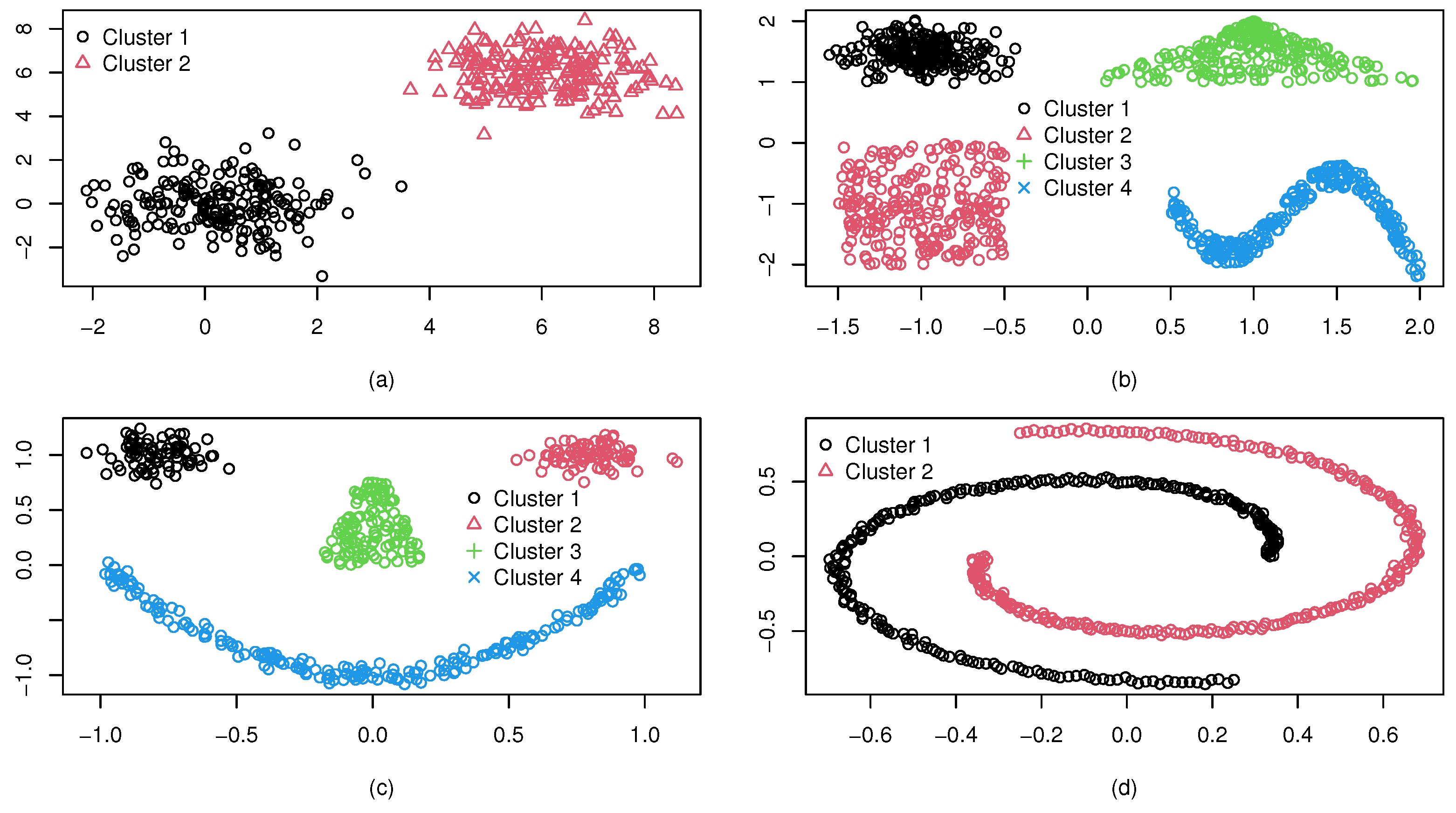
We consider some synthetic datasets with cluster shapes different from an ellipsoid, and denote them as $D_1$. The dataset $D_1$(a) consists of two isolated clusters, each with 200 observations generated from Gaussian distributions. Dataset $D_1$(b) consists of four isolated clusters with different shapes: elliptical, triangular, rectangular, and wave. In dataset $D_1$(c), there are also four isolated clusters of different shapes. However, the ellipsoid boundaries are not fully isolated, unlike the case in dataset $D_1$(b). Dataset $D_1$(d) contains two spiral clusters each of 250 observations. All the synthetic datasets are in two dimensions, which were randomly generated by using the package “‘mlbench’” in R. Figure 4 shows the four synthetic datasets, and it can be seen that the cluster numbers of $D_1$(a)–(d) are 2, 4, 4, and 2, respectively.

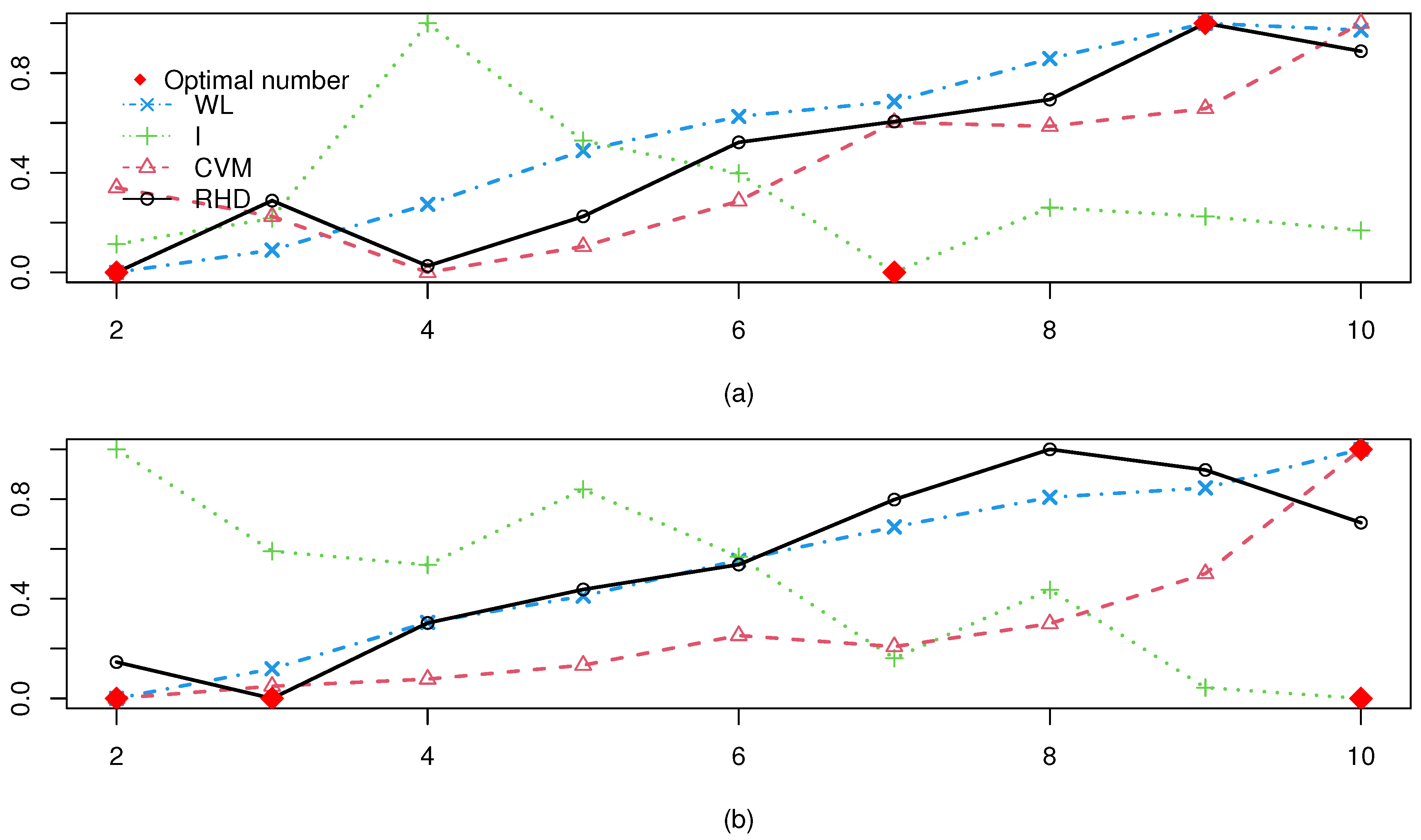
To address the substantial discrepancies in results generated by different indices and enable their visualization within a unified coordinate system, we applied Min–Max normalization (Equation (25)) to the outputs. This transformation scales all index values into the $[0,1]$ interval while preserving the original ordinal relationships between values. By maintaining the relative ordering of scores, this preprocessing step facilitates direct comparative analysis across indices with distinct magnitude ranges, ensuring consistent interpretation within the standardized scale.

$$z={\displaystyle \frac{x-min\left\{x\right\}}{max\left\{x\right\}-min\left\{x\right\}}},$$

(25)

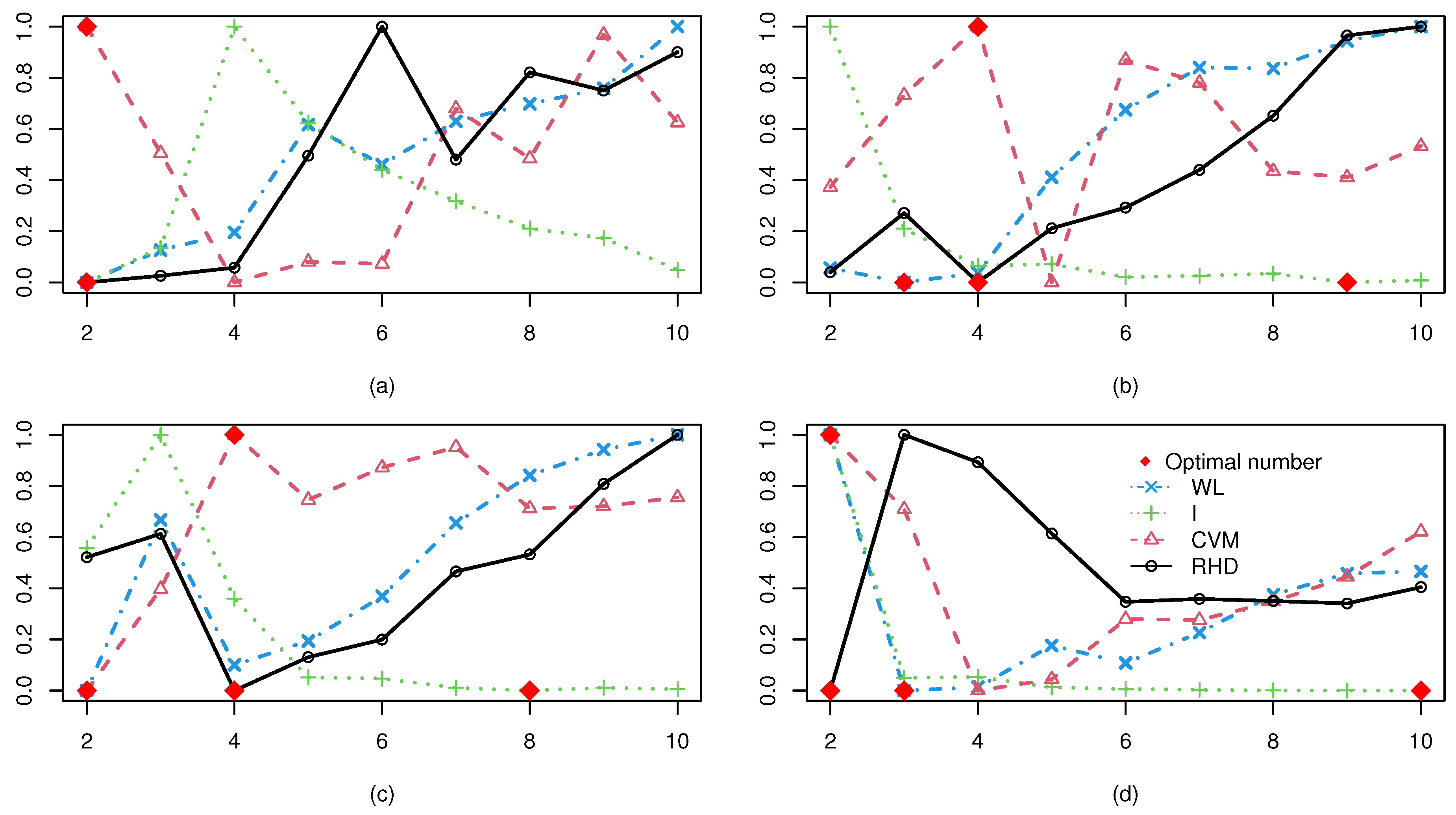
To eliminate clustering randomness, each experiment was repeated ten times, with the average results. Figure 5 displays WL, I, CVM, and RHD index values from spectral clustering with varying cluster numbers for $D_2$(a)–(d). The optimal cluster count for each CVI is marked by a red diamond. Analysis shows that the RHD and CVM indices exhibit consistent reliability across all datasets, accurately identifying the true cluster numbers as 2, 4, 4, and 2 for $D_2$(a)–(d), respectively. This precision aligns with the ground-truth structures. In contrast, the WL and I indices achieve comparable accuracy only for $D_2$(a), but fail to determine optimal partitions for the other three datasets. These results highlight RHD and CVM’s superior adaptability to complex scenarios, particularly for non-convex distributions and varying dimensionality in the $D_2$ series. This also proves that the WL and the I-index are only suitable for ellipsoidal clusters, even when well separated.

Table 1. Comparison of classification accuracy rate (%) for different CVIs under datasets $D_1$(a)–(d).

Dataset	CVI
	WL	I	CVM	RHD
$D_1$(a)	100.00	100.00	100.00	100.00
$D_1$(b)	75.00	64.00	100.00	100.00
$D_1$(c)	50.00	64.80	100.00	100.00
$D_1$(d)	86.80	60.60	100.00	100.00

evaluates the classification accuracy (%) of four CVIs—WL, I, CVM, and RHD—applied to dataset $D_1$(a)–(d). Key findings reveal a distinct performance hierarchy: CVM and RHD achieved 100% accuracy across all $D_1$ variants, demonstrating robust adaptability to diverse data characteristics. In contrast, performance disparities emerged among other indices. While all CVIs attained 100% accuracy in $D_1$(a) (indicating ideal separability), the subsequent variants exposed limitations. Specifically, WL accuracy exhibited a V-shaped trend, declining from 75.00% ($D_1$(b)) to 50.00% ($D_1$(c)) before recovering to 86.80% ($D_1$(d)). Index I displayed marked instability, oscillating between 60.60% ($D_1$(d)) and 64.80% ($D_1$(c)) with an intermediate value of 64.00% ($D_1$(b)). Notably, the synergy between FSDP and CVM/RHD produced flawless classifications even in complex scenarios like $D_1$(c), where WL and I indices’ accuracy dropped below 65%. This underscores their enhanced resilience to challenges such as non-convex boundaries and noise interference. Collectively, these results highlight the critical role of CVI selection in ensuring algorithmic reliability.

5.1.2. Overlapped Datasets

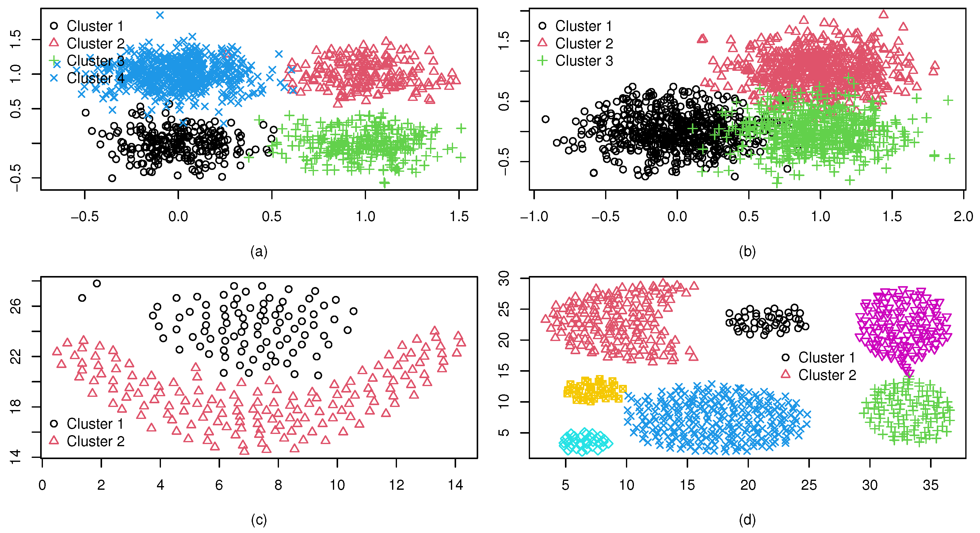
In the preceding section, we rigorously demonstrated the exceptional discriminative capability of both CVM and the proposed RHD index for well-separated clusters. Building on this foundation, a more challenging question arises: whether RHD and CVM maintain proficiency in determining optimal cluster numbers when handling overlapping data distributions. This question directly investigates the robustness of the novel index under non-ideal conditions, specifically its ability to overcome the limitations of conventional validity measures that falter in detecting overlapping structures. Resolving this issue is pivotal for validating the algorithm’s practical applicability in complex real-world scenarios with compromised data separability.

Figure 6 presents four synthetic datasets with varying degrees of cluster overlap, designated as $D_2$(a)–(d). The first two datasets, $D_2$(a) and $D_2$(b), were algorithmically generated using stochastic sampling techniques to simulate controlled overlap scenarios. Specifically, $D_2$a comprises four clusters with moderate pairwise overlaps, as visualized in Figure 6a, while $D_2$(b) (panel b) contains three clusters with highly complex inter-cluster boundaries and significant overlap regions. The latter two datasets, $D_2$(c)–(d), were selected from established clustering datasets https://github.com/milaan9/Clustering-Datasets (accessed on 15 June 2025) benchmarks to introduce real-world complexity. Dataset $D_2$(c) (Figure 6c) corresponds to the renowned “Frame” structure, featuring a flame-like bimodal distribution with ambiguous decision boundaries between two elongated clusters. Of particular interest is dataset $D_2$(d) (Figure 6d), the aggregation benchmark, which consists of seven clusters with heterogeneous geometries: a crescent moon, dual balloon-shaped clusters, and four ellipsoidal clusters of varying sizes and densities. This configuration introduces substantial overlaps between adjacent clusters while preserving distinct morphological features, creating a challenging validation scenario for clustering validity indices.

Table 2. The estimated number of clusters based on different CVIs under four overlapped datasets $D_2$(a)–$D_1$(d).

Dataset	$\#\mathit{C}$	Index
		WL	I	CVM	RHD
$D_2\left(a\right)$	4	$3^6,2^4$	${\mathbf{4}}^{\mathbf{10}}$	${10}^5,9^2,7^3$	${\mathbf{4}}^{\mathbf{10}}$
$D_2\left(b\right)$	3	$2^{10}$	${10}^8,9^2$	${10}^6,9^4$	${\mathbf{3}}^{\mathbf{8}},2^2$
$D_2\left(c\right)$	2	${\mathbf{2}}^{\mathbf{10}}$	$2^9,4^1$	${10}^8,9^2$	${\mathbf{2}}^{\mathbf{10}}$
$D_2\left(d\right)$	7	$2^{10}$	$9^4,{\mathbf{7}}^{\mathbf{3}},8^2$	$5^4,9^3,6^2,{\mathbf{7}}^{\mathbf{1}}$	$5^{10}$
Accuracy rate		25.00%	32.50%	2.50%	70%
95% confidence intervals		(11.57%, 38.43%,)	(18.02%, 46.98%)	(0%,7.34%)	(55.79%, 84.22%)

“#C” means the true number of clusters.

summarizes the clustering validity results for datasets $D_2$(a)–(d), with $\#C$ denoting the ground-truth cluster count. The boldfaced values indicate correctly identified optimal cluster counts. In Table 2, all experiments were repeated 10 times; the notation $a^b$ represents the algorithm’s determination that a is the optimal cluster number in b out of 10 independent trials. For instance, regarding dataset $D2\left(a\right)$, the notation $3^6,2^4$ under the WL index indicates that, across 10 experiments, the WL index determined the optimal number of clusters as three in six cases and as two in four cases.

The analysis of results presented in Table 2 reveals that for the $D_2$(a) dataset, both the I index and RHD correctly identified the true cluster count (four clusters). This demonstrates their superior discriminative ability for ellipsoid-shaped clusters with mild overlaps, where conventional metrics may struggle with boundary ambiguity. The consistent success across 10 trials (10/10 for I and RHD) underscores their robustness in this scenario. For the $D_2$(b) dataset: This highly overlapping dataset (three clusters) posed significant challenges. RHD achieved remarkable performance with 8/10 correct identifications, while all other indices failed completely. This highlights RHD’s enhanced capability to resolve complex decision boundaries in densely overlapping structures, a critical advantage over existing metrics. For the $D_2$(c) dataset (Frame): The flame-like bimodal distribution with ambiguous boundaries was accurately resolved by WL and RHD (both 10/10). Conversely, I and CVM failed to detect the correct two-cluster structure, indicating their sensitivity to elongated, non-convex geometries where density gradients become critical. For the $D_2$(d) dataset (Aggregation): This heterogeneous benchmark (seven clusters) introduced morphological diversity and varying overlaps. Interestingly, I demonstrated partial success (3/10) by occasionally capturing dominant density patterns, while RHD and WL failed completely. CVM’s rare success (1/10) suggests its susceptibility to noise in multi-scale cluster configurations. This dataset exposes limitations of all the indices in highly heterogeneous environments.

As evidenced by the cross-algorithm accuracy comparisons in Table 2, the proposed RHD index consistently outperforms existing metrics, achieving 70.00% overall accuracy (28/40 cases)—a 37.5 percentage point improvement over the suboptimal I index (32.50%). While the WL index ranked third (25.00%), the CVM metric exhibited severe limitations in resolving non-linear manifold structures, attaining only 2.50% accuracy. This stark contrast underscores the vulnerability of CVM’s feature-space partitioning strategy to local optima within high-dimensional, geometrically complex data regimes.

The experiments reveal RHD’s exceptional versatility across mild-to-severe cluster overlaps and geometric complexities. Its superior performance in $D_2$(b) and $D_2$(c) validates its robustness to boundary ambiguity and non-convex structures. While Index I exhibits niche strengths in specific morphologies ($D_2$(a) and $D_2$(d)), Index I’s inconsistency across datasets contrasts with RHD’s reliable pattern recognition. These findings underscore RHD’s potential for real-world clustering challenges with compromised data separability, offering significant methodological advances over traditional validity indices.

Based on the cross-dataset results in Table 2, the RHD index exhibits significant advantages in low-to-moderate overlap scenarios (e.g., 100% correct identification in $D_2$(a)). Crucially, in the highly overlapping $D_2$(d), it maintains an 80% correct identification rate. Although Index I matches RHD’s performance in simple structures ($D_2$(a)), its discriminative ability deteriorates significantly with increasing data complexity ($D_2$(c)–(d)). This contrast highlights RHD’s robustness to inter-cluster boundary ambiguity, with its core advantage lying in joint modeling of the local density and global separation.

However, RHD exhibits a key limitation in hybrid cluster structures, when datasets contain both well-separated clusters and overlapping clusters (e.g., the aggregation structure $D_2$(d)), as this index tends to over-merge overlapping regions. Mechanism analysis reveals that this phenomenon stems from the definition of the inter-class difference measure $S_{RHD}$. Specifically, $S_{RHD}$ yields higher values for well-separated clusters but decreases significantly for overlapping clusters. When both types coexist, the global mean $S_{RHD}$ is depressed by low-value overlapping regions; according to the $S_{RHD}$ formula, a reduced denominator s inversely amplifies the index value. Consequently, the algorithm mistakenly believes merging overlapping clusters improves clustering quality. The failure of CVM arises because increasing cluster counts shrink $d_{\mathrm{bad}\mathrm{hbox}}\left(j\right)$, causing the compactness $R_{\mathrm{in}}\left(j\right)$ to rise progressively. This ultimately elevates the CVM values. Since larger CVM values indicate better clustering, the cluster number may be overestimated.

5.2. Experiments on Real Datasets

In the final chapter, we thoroughly expanded the systematic evaluation of the proposed RHD index against benchmark methods for two scenarios: sufficient class separation and class overlap. Crucially, the combined effects of convex and non-convex data distributions were rigorously examined under both experimental paradigms. Multidimensional simulations revealed that these combined effects significantly influenced most test scenarios, with the RHD index demonstrating superior clustering validity assessment. To ensure a comprehensive scope, real-world datasets were analyzed alongside synthetic ones.

In view of the large-scale, high-dimensional, and multi-category characteristics of real-world scene data, the following experiments will focus on classical benchmark datasets to systematically examine these features and their interactions.

Firstly, we considered two public benchmark datasets: Iris and Seeds, sourced from the UCI database [21]. The Iris dataset comprises three classes with 50 instances each, where one class is linearly separable from the other two. The Seeds dataset contains 210 measurements of kernel geometrical properties from three wheat varieties, with each group approximately Gaussian-distributed.

Secondly, we evaluate the proposed index on three high-dimensional real-world datasets exemplifying complex data characteristics. The Ionosphere dataset, collected by a phased-array radar system in Goose Bay, Labrador, comprises 351 instances with 15 features encoding ionospheric reflection properties. The Landsat Satellite Imagery dataset contains 2000 multispectral images across 36 spectral bands, capturing terrestrial surface characteristics in visible and infrared wavelengths. The Yeast dataset, widely used for predicting protein cellular localization sites, contains 10 localization categories. All datasets are publicly accessible via the UCI Machine Learning Repository (https://archive.ics.uci.edu/datasets, accessed on 15 June 2025) and present distinct challenges: Ionosphere exhibits moderate dimensionality with limited samples, while Landsat features high-dimensional spectral measurements with inherent non-linear structures. These properties establish them as ideal benchmarks for validating clustering validity indices under real-world conditions.

Lastly, the Face dataset is publicly accessible via https://www.mcm.edu.cn/html_cn/block/8579f5fce999cdc896f78bca5d4f8237.html (accessed on 15 June 2025), containing 20 facial images from two individuals under varying lighting conditions. Featuring 2016 dimensions—significantly exceeding the sample size—this dataset is characterized as high-dimensional. Summary statistics for all five real datasets are provided in

Table 3. Characteristics of the five real datasets.

Dataset	Sizes	Features	$\#\mathit{C}$
Iris	150	4	3
Seeds	210	7	3
Ionosphere	315	15	2
Landsat	2000	36	6
Yeast	1484	8	10
Face	20	2016	2

“#C” means the true number of clusters.

.

Figure 7 presents the WL, I, CVM, and RHD values for varying cluster numbers K across both real datasets. The optimal value for each CVI is marked with a red diamond. The RHD index correctly determined the cluster count for one dataset (Seeds). Although it misidentified the number as 2 for Iris, this result remains close to the true count. In contrast, the other three CVIs failed completely on all real datasets.

Table 4. The WL, CVM, and RHD values performed on the Ionosphere dataset.

K	CVIs
	WL	I	CVM	RHD
2	0.503	7.87 $\times {10}^{-2}$	4.304	9.611
3	0.674	5.78 $\times {10}^{-4}$	10.614	15.389
4	0.649	2.63 $\times {10}^{-4}$	13.557	14.066
5	0.974	8.89 $\times {10}^{-5}$	22.894	14.822
6	0.898	2.63 $\times {10}^{-4}$	47.835	19.089
7	0.926	2.12 $\times {10}^{-4}$	44.086	21.543
8	0.981	2.50 $\times {10}^{-5}$	158.272	23.579
9	0.980	2.14 $\times {10}^{-5}$	221.264	28.056
10	0.949	1.68 $\times {\mathbf{10}}^{-\mathbf{5}}$	229.242	28.805

,

Table 5. The WL, CVM, and RHD values performed on the Landsat dataset.

K	CVIs
	WL	I	CVM	RHD
2	0.314	449.141	6619.049	5.851
3	0.184	383.355	16,677.85	4.868
4	0.381	347.097	27,907.302	6.713
5	0.442	240.779	34,106.170	6.325
6	0.570	283.063	52,052.447	4.147
7	0.715	232.062	62,217.019	8.289
8	0.685	123.809	78,623.222	11.147
9	0.980	298.980	99,568.877	15.365
10	0.790	192.983	122,083.103	17.318

,

Table 6. The WL, CVM, and RHD values performed on the Yeast dataset.

K	CVIs
	WL	I	CVM	RHD
2	0.144	1.68 $\times {\mathbf{10}}^{-\mathbf{6}}$	0.673	12.031
3	0.547	1.13 $\times {10}^{-4}$	0.067	11.531
4	0.762	2.76 $\times {10}^{-4}$	0.072	20.503
5	0.813	8.02 $\times {10}^{-5}$	0.207	15.171
6	1.011	2.21 $\times {10}^{-4}$	0.182	21.127
7	0.939	1.69 $\times {10}^{-4}$	0.400	21.182
8	1.030	2.13 $\times {10}^{-4}$	0.546	22.749
9	1.000	1.11 $\times {10}^{-4}$	0.605	26.632
10	1.138	9.39 $\times {10}^{-5}$	0.608	33.421
11	0.699	1.49 $\times {10}^{-5}$	1.682	36.726
12	1.183	1.25 $\times {10}^{-4}$	0.858	40.998
13	1.094	1.02 $\times {10}^{-5}$	2.665	50.258
14	1.065	7.74 $\times {10}^{-5}$	2.062	44.517
15	1.149	2.23 $\times {10}^{-5}$	1.664	63.840

and

Table 7. The WL, CVM, and RHD performed on the Faces dataset.

K	CVIs
	WL	I	CVM	RHD
2	0.0003	/	12,878,003	0.4906
3	0.0023	/	6,846,685	0.7017
4	0.0026	/	14,017,945	0.9195
5	0.0036	/	22,351,889	0.7426
6	0.0042	/	25,110,017	0.8364
7	0.00296	/	23,237,725	0.923
8	0.00296	/	22,265,433	0.832
9	0.00296	/	26,132,821	0.977
10	0.00296	/	27,589,721	1.232

summarize the mean performance (over 10 repetitions) of four clustering validity indices evaluated on four benchmark datasets: Ionosphere, Landsat satellite imagery, Yeast gene expression, and Faces. Table 4 (classic Iris dataset analysis) reveals that both the WL index and our proposed RHD index identified two clusters, whereas the I and CVM indices detected 10 clusters (indicating structural complexity overestimation). This discrepancy stems from the Iris dataset’s intrinsic properties: the Virginica class is well-separated in feature space, but Setosa and Versicolor exhibit substantial overlap, reflecting a partially overlapping cluster structure. Furthermore, experiments on the synthetic dataset $D_2\left(d\right)$ (designed with hybrid cluster separation-overlap patterns) corroborate that the RHD index systematically underestimates the true cluster count in mixed scenarios with coexisting distinct and overlapping clusters.

As shown in Table 5, the RHD index exclusively achieved perfect alignment with the six ground-truth land cover types in Landsat’s 36-dimensional spectral feature space. Validation on the facial image dataset (Table 7) revealed that both WL and RHD indices correctly identified two distinct facial identities (each with multiple pose variations), demonstrating efficacy in modeling complex image manifolds. In contrast, the CVM index consistently overestimated cluster counts (predicting 10 clusters), highlighting limitations in high-dimensional feature-space partitioning. The I index failed critically due to non-invertible covariance matrices—a known computational challenge when processing ultra-high-dimensional data like facial features.

The experimental results on the Yeast dataset (Table 6) revealed consistent failure of all four clustering validity indices to detect intrinsic functional modules, underscoring fundamental limitations of traditional evaluation paradigms in addressing domain-specific complexity. These results collectively emphasize that current clustering assessment frameworks face critical challenges in interpreting biological systems—systems inherently governed by emergent self-organization, functional redundancy, and multiscale invariance. To bridge this gap, future methodologies may necessitate hybrid strategies integrating biologically informed constraints (e.g., gene ontology-driven feature embeddings) with advanced geometric tools such as persistent homology from topological data analysis (TDA) to capture multiscale hierarchical structures.

As summarized in

Table 8. The estimated number of clusters based on different CVIs under real datasets over 10 experiments.

Dataset	$\#\mathit{C}$	Index
		WL	I	CVM	RHD
Iris	4	$2^{10}$	$6^7,2^4$	$9^7,8^2,{10}^1$	$2^8,{\mathbf{3}}^{\mathbf{2}}$
Seeds	3	$2^7,{\mathbf{3}}^{\mathbf{3}}$	${10}^6,7^3$	${10}^9,9^4$	${\mathbf{3}}^{\mathbf{9}},2^1$
Ionosphere	2	${\mathbf{2}}^{\mathbf{10}}$	${10}^6,9^3,8^1$	${10}^8,9^2$	${\mathbf{2}}^{\mathbf{10}}$
Landsat	7	$3^8,2^2$	$8^8,7^2$	${10}^{10}$	${\mathbf{6}}^{\mathbf{6}},3^4$
Yeast	7	$2^{10}$	$2^{10}$	${13}^5,{14}^3,{11}^1,{10}^1$	$3^6,2^5$
Face	7	${\mathbf{2}}^{\mathbf{10}}$	/	${10}^7,9^2,6^1$	${\mathbf{2}}^{\mathbf{10}}$
Accuracy rate		38.33%	0.00%	1.67%	61.67%
95% confidence intervals		(26.02%, 50.64%)	(0.00%, 0.00%)	(0.00%, 4.90%)	(49.38%, 73.69%)

“#C” means the true number of clusters.

, the RHD index significantly outperformed other indices in cluster count estimation, achieving 61.67% accuracy (37/60 correct identifications) across 60 trials—a 23.33% improvement over the second-best WL index (38.33%). Its peak accuracy (100%) on datasets with well-defined manifold structures (e.g., Landsat satellite imagery and Faces) confirms the robustness of its density-sensitive manifold learning framework. Conversely, traditional methods revealed critical limitations: the CVM index showed near-random performance (one success in synthetic data), and the I index failed completely in ultra-high-dimensional biological domains (e.g., Yeast gene expression) due to non-invertible covariance matrices. These failures underscore the inadequacy of Euclidean-centric metrics for non-linear topological spaces and high-dimensional pathological conditions.

Notably, all four indices, including the proposed one, failed to identify the true number of clusters in the Yeast dataset. The primary reason is that the expression levels of yeast genes exhibit continuous gradation during biological processes (e.g., cell cycle, metabolic regulation) rather than discrete cluster-like distributions. Specifically, there are no clear boundaries between clusters. While the new index can effectively recognize clusters with low overlap, it still cannot accurately identify such continuously gradational cluster distributions. This also represents a major challenge in the recognition of biological images, gene data, and similar datasets, warranting more in-depth research on such data in future studies.

6. Conclusions

Determining the optimal number of clusters remains a critical yet unresolved challenge in unsupervised learning, as prevailing cluster validity indices (CVIs) often exhibit context-dependent limitations. Despite extensive efforts to develop CVIs for specific clustering scenarios (e.g., spherical or linearly separable clusters), their generalizability to complex real-world data, characterized by unknown cluster geometries, density heterogeneity, and partial overlaps, remains questionable. To bridge this gap, we propose a novel density-aware CVI based on the density peak hypothesis [1], which mitigates the inherent limitations of Euclidean-based metrics regarding centroid instability under noise and outlier interference.

The proposed Robust Hierarchical Distance (RHD) index introduces a paradigm shift by replacing conventional pairwise Euclidean distances with minimal separation distances to higher-density neighbors, effectively decoupling compactness measurement from cluster morphology. This innovation enables the RHD index to adaptively quantify intra-cluster cohesion while remaining invariant under non-convex topologies and density fluctuations. Theoretical analysis confirms its resilience to proximal cluster centers and skewed distributions, overcoming the “centration bias” inherent in centroid-based CVIs.

Comprehensive experiments using synthetic and real datasets evaluated diverse scenarios, including overlapping clusters, irregular shapes, density variations, and proximal cluster centroids. The results demonstrate a 23–32% improvement in accuracy for cluster count estimation over state-of-the-art cluster validity indices (CVIs).

Although the RHD index exhibits its ability in specific scenarios, it also has two key limitations: high computational complexity due to multiple local density comparisons and distance calculations (especially for large datasets), and poor performance in identifying clusters with indistinct density differences (e.g., Yeast dataset) or continuous gradient changes, as it relies on distinct density variations for partitioning. Future work will optimize algorithm structure (e.g., using approximate nearest neighbor search) to reduce complexity and improve density measurement by incorporating continuous gradient-capturing mechanisms and domain knowledge to enhance adaptability to complex data.

References

1. Rodriguez, A.; Laio, A. Clustering by fast search and find of density peaks. Science 2014, 344, 1492–1496. [Google Scholar] [CrossRef] [PubMed]
2. Wu, G.; Zhao, X.; Luo, S.; Shi, H. Histological image segmentation using fast mean shift clustering method. Biomed. Eng. Online 2015, 14, 24. [Google Scholar] [CrossRef] [PubMed]
3. Fujita, A.; Takahashi, D.Y.; Patriota, A.G. A non-parametric method to estimate the number of clusters. Comput. Stat. Data Anal. 2014, 73, 27–39. [Google Scholar] [CrossRef]
4. Dunn, J.C. A fuzzy relative of the ISODATA process and its use in detecting compact well-separatedclusters. J. Cybern. 1974, 3, 32–57. [Google Scholar] [CrossRef]
5. Bezdek, J.C. Cluster validity with fuzzy sets. J. Cybern. 1973, 3, 58–73. [Google Scholar] [CrossRef]
6. Xie, X.L.; Beni, G. A validity measure for fuzzy clustering. IEEE Trans. Pattern Anal. Mach. Intell. 1991, 13, 841–847. [Google Scholar] [CrossRef]
7. Gindy, N.; Ratchev, T.; Case, K. Component grouping for GT applications—A fuzzy clustering approach with validity measure. Int. J. Prod. Res. 1995, 33, 2493–2509. [Google Scholar] [CrossRef]
8. Pakhira, M.K.; Bandyopadhyay, S.; Maulik, U. Validity index for crisp and fuzzy clusters. Pattern Recognit. 2004, 37, 487–501. [Google Scholar] [CrossRef]
9. Wu, C.H.; Ouyang, C.S.; Chen, L.W.; Lu, L.W. A new fuzzy clustering validity index with a median factor for centroid-based clustering. IEEE Trans. Fuzzy Syst. 2015, 23, 701–718. [Google Scholar] [CrossRef]
10. Said, A.B.; Hadjidj, R.; Foufou, S. Cluster validity index based on Jeffrey divergence. Pattern Anal. Appl. 2017, 20, 21–31. [Google Scholar] [CrossRef]
11. Morsier, F.D.; Tuia, D.; Borgeaud, M.; Gass, V.; Thiran, J.P. Cluster validity measure and merging system for hierarchical clustering considering outliers. Pattern Recognit. 2015, 48, 1478–1489. [Google Scholar] [CrossRef]
12. Hruschka, E.R.; Campello, R.J.G.B.; Freitas, A.A. A survey of evolutionary algorithms for clustering. IEEE Trans. Syst. Man Cybern. Part C 2009, 39, 133–155. [Google Scholar] [CrossRef]
13. Everitt, B.S.; Landau, S.; Leese, M.; Stahl, D. Miscellaneous clustering methods. In Cluster Analysis, 5th ed.; John Wiley & Sons: Hoboken, NJ, USA, 2011; pp. 215–255. [Google Scholar]
14. Celeux, G.; Govaert, G. A classification EM algorithm for clustering and two stochastic versions. Comput. Stat. Data Anal. 1992, 14, 315–332. [Google Scholar] [CrossRef]
15. Tibshirani, R.; Walther, G.; Hastie, T. Estimating the Number of Clusters in a Data Set via the Gap Statistic. J. R. Stat. Soc. 2001, 63, 411–423. [Google Scholar] [CrossRef]
16. Fang, Y.; Wang, J. Selection of the number of clusters via the bootstrap method. Comput. Stat. Data Anal. 2012, 56, 468–477. [Google Scholar] [CrossRef]
17. Bezdek, J.C. Numerical taxonomy with fuzzy sets. J. Math. Biol. 1974, 1, 57–71. [Google Scholar] [CrossRef]
18. Xu, Y.; Srinivasan, A.; Xue, L. A selective overview of recent advances in spectral clustering and their applications. In Modern Statistical Methods for Health Research; Springer: Berlin/Heidelberg, Germany, 2021; pp. 247–277. [Google Scholar]
19. Wu, S.; Feng, X.; Zhou, W. Spectral clustering of high-dimensional data exploiting sparse representation vectors. Neurocomputing 2014, 135, 229–239. [Google Scholar] [CrossRef]
20. Li, Y.; He, K.; Kloster, K.; Bindel, D.; Hopcroft, J. Local spectral clustering for overlapping community detection. ACM Trans. Knowl. Discov. Data (TKDD) 2018, 12, 1–27. [Google Scholar] [CrossRef]
21. Bache, K.; Lichman, M. UCI Machine Learning Repository. 2013. Available online: http://archive.ics.uci.edu/ml (accessed on 15 June 2025).
Figure 1. Traditional and new calculation of compactness within a cluster and separation between clusters.
Axioms 14 00578 g001
Figure 2. Boxplot of neighborhood distance based on Euclidean distance, Mahalannobis distance and Manhattan distance.
Axioms 14 00578 g002
Figure 3. Running time.
Axioms 14 00578 g003
Figure 4. Four well-separated synthetic datasets D 1 : (a) two normally-shaped clusters; (b) four clusters with isolated boundaries; (c) four clusters with ellipsoid boundaries not fully isolated; and (d) two spiral clusters.
Axioms 14 00578 g004
Figure 5. The WL, I, CVM, and RHD values with different number of clusters under the synthetic dataset: (a) Dataset D 1 (a); (b) Dataset D 1 (b); (c) Dataset D 1 (c); (d) Dataset D 1 (d).
Axioms 14 00578 g005
Figure 6. Four overlapped datasets: (a) Dataset D 2 (a); (b) Dataset D 2 (b); (c) Dataset D 2 (c); (d) Dataset D 2 (d).
Axioms 14 00578 g006
Figure 7. Test results of two real datasets: (a) Iris; (b) Seeds.
Axioms 14 00578 g007