Self-Normalized Large Deviation Principle and Cramér Type Moderate Deviations for a Supercritical Branching Process

Abstract

Let ${\left(Z_n\right)}_{n\ge 0}$ be a supercritical branching process with offspring distribution $p_r=\mathbb{P}(Z_1=r),r\ge 0,$ such that $p_0=p_1=\dots =p_{k_0-1}=0$ and $p_{k_0}>0$, where $k_0\ge 2$. The Lotka–Nagaev estimator $Z_{n+1}/Z_n$ is an important estimator for the offspring mean $m={\sum }_{i=k_0}^{\infty }i{p}_i$. In this paper, we establish a self-normalized large deviation result and self-normalized Cramér type moderate deviations for the Lotka–Nagaev estimator. An application to constructing confidence intervals for m is also discussed.

1. Introduction

A branching process can be described as follows: for all $n\ge 0$,

$$Z_0=1,Z_{n+1}=\sum _{i=1}^{Z_n}{X}_{n,i},$$

(1)

where $X_{n,i}$ stands for the offspring number of the i-th individual of the generation n. We assume that the random variables ${\left(X_{n,i}\right)}_{i\ge 1}$ are independent of each other and share a common distribution law as follows:

$$\mathbb{P}(X_{n,i}=r)=p_r,r\ge 0.$$

(2)

Moreover, they are also independent of $Z_1,Z_2,...,Z_n$. An important task for the branching processes is to estimate the offspring mean m of an individual. Clearly, it holds

$$m=\mathbb{E}{Z}_1=\mathbb{E}{X}_{n,i}=\sum _{r=1}^{\infty }r{p}_r.$$

All over the paper, we assume that $p_0=0$ and denote $k_0=inf\{j:j\ge 2,p_j\ne 0\}$, which means each individual has at least $k_0$ offsprings. To avoid the deterministic case, we also assume that $0<p_{k_0}<1.$ The Lotka–Nagaev [1,2] estimator $Z_{n+1}/Z_n$ is an important estimator for the estimation of the offspring mean m. It is obvious that $Z_n\to \infty$ almost surely (a.s.) as $n\to \infty$. Thus, according to the strong law of large numbers, it holds as $n\to \infty$,

$${\displaystyle \frac{Z_{n+1}}{Z_n}}\to ma.s.$$

Thus, the Lotka–Nagaev estimator is well defined $\mathbb{P}$-a.s.

For the branching processes, Athreya [3] has established large deviation principles for the normalized Lotka–Nagaev estimator; Ney and Vidyashankar [4,5] and He [6] obtained some rate estimates for the large deviations of the Lotka–Nagaev estimator; Bercu and Touati [7] gave some exponentially large deviation inequalities for the Lotka–Nagaev estimator with self-normalized martingale methods. When $k_0=1$, Chu [8] has established a sharp self-normalized large deviation result, see also Fan and Shao [9,10] for self-normalized Cramér type moderate deviations for the weighted Lotka–Nagaev estimator. Recently, Doukhan et al. [11] obtained some standardized Cramér moderate deviations for the Lotka–Nagaev estimator. Cramér moderate deviations have attracted a lot of attention. We refer to Petrov [12], Beknazaryan, Sang and Xiao [13], Fan and Shao [14] for such results. For the self-normalized Cramér type moderate deviations, we refer to Jing et al. [15], Fan, Hu and Xu [16] and Fan and Shao [9]. The advantage of self-normalized Cramér moderate deviations lays in the fact that it adopts to the case that the variances of random variables are unknown.

Despite the fact that the Lotka–Nagaev estimator is well studied, there is no result for self-normalized large deviation principles and Cramér type moderate deviations for the Lotka–Nagaev estimator, provided that $k_0>1$. The main goal of this paper is to fill this gap.

The paper is organized as follows: In Section 2, we present a self-normalized large deviation principle result and some self-normalized Cramér type moderate deviations for the Lotka–Nagaev estimator, provided that $k_0>1$. In Section 3, we give an application of self-normalized Cramér type moderate deviations to constructing confidence intervals of m. The remaining sections in the paper are devoted to the proofs of theorems and their corollaries.

2. Main Results

The following theorem gives a self-normalized large deviation principle for supercritical branching processes in the case that $p_0=p_1=\dots =p_{k_0-1}=0$ and $p_{k_0}>0$ for some $k_0\ge 2$.

Theorem 1.  

Assume $p_0=p_1=0$ and let $k_0=inf\{j:j\ge 2,p_j\ne 0\}$. For all $x>0$, then there exists $\lambda \left(x\right)\in (0,\infty ]$ such that

$$\underset{n\to \infty }{lim\; sup}{\displaystyle \frac{1}{k_0^n}}ln\mathbb{P}\left({\displaystyle \frac{\sqrt{Z_n}}{\sqrt{{\sum }_{i=1}^{Z_n}{\left(X_{n,i}-\frac{Z_{n+1}}{Z_n}\right)}^2}}}\left|{\displaystyle \frac{Z_{n+1}}{Z_n}}-m\right|\ge x\right)\le -\lambda \left(x\right).$$

(3)

Remark 1.  

Some remarks on Theorem 1 follow.

1. 

Assume the conditions of Theorem 1. Ney and Vidyashankar [5] have established the following large deviation result: If $\mathbb{E}[exp\left\{\theta Z_1\right\}]<\infty$ for some constant $\theta >0$, then there exists $\tilde{\lambda }\left(x\right)\in (0,\infty ]$ such that for all $x>0$,

$$\underset{n\to \infty }{lim\; sup}{\displaystyle \frac{1}{k_0^n}}ln\mathbb{P}\left(\left|{\displaystyle \frac{Z_{n+1}}{Z_n}}-m\right|\ge x\right)\le -\tilde{\lambda }\left(x\right).$$

(4)

Obviously, Theorem 1 gives an extension of the last result to the self-normalized case. Compared with the last result (4), Theorem 1 holds without the moment generating function.

2. 

Assume that $p_0=0$ and $0<p_1<1$. Ney and Vidyashankar [5] proved that if $\mathbb{E}[exp\left\{\theta Z_1\right\}]<\infty$ for some constant $\theta >0$, then there exists a positive function $p\left(x\right)$ such that it holds for all $x>0$,

$$\underset{n\to \infty }{lim}{\displaystyle \frac{1}{p_1^n}}ln\mathbb{P}\left(\left|{\displaystyle \frac{Z_{n+1}}{Z_n}}-m\right|\ge x\right)=p\left(x\right)<\infty .$$

(5)

For the explicit expression of $p\left(x\right)$, we refer to Ney and Vidyashankar [5]. Chu [8] obtained a self-normalized version of (5): There exists a function $q\left(x\right)$ such that it holds for all $x>0$,

$$\underset{n\to \infty }{lim}{\displaystyle \frac{1}{p_1^n}}ln\mathbb{P}\left({\displaystyle \frac{\sqrt{Z_n}}{\sqrt{{\sum }_{i=1}^{Z_n}{\left(X_{n,i}-\frac{Z_{n+1}}{Z_n}\right)}^2}}}\left|{\displaystyle \frac{Z_{n+1}}{Z_n}}-m\right|\ge x\right)=q\left(x\right)<\infty .$$

(6)

For the explicit expression of $q\left(x\right)$, we refer to Theorem 1 of Chu [8].

Assume that the random variables ${\left(X_{n,i}\right)}_{1\le i\le Z_n}$ can be observed. Let

$$T_n={\displaystyle \frac{Z_n\left(\frac{Z_{n+1}}{Z_n}-m\right)}{\sqrt{{\sum }_{i=1}^{Z_n}{\left(X_{n,i}-\frac{Z_{n+1}}{Z_n}\right)}^2}}}$$

(7)

be the t-statistic for the Lotka–Nagaev estimator ${\displaystyle \frac{Z_{n+1}}{Z_n}}$. Denote $\mathsf{\Phi }\left(x\right)$ the standard normal distribution function. We have the following self-normalized Cramér type moderate deviations for $T_n$.

Theorem 2.  

Assume $p_0=p_1=0$ and let $k_0=inf\{j:j\ge 2,p_j\ne 0\}$. If $\mathbb{E}{Z}_1^{2+\rho }<\infty$ for some $\rho \in (0,1]$, then it holds

$$\left|ln{\displaystyle \frac{\mathbb{P}\left(T_n\ge x\right)}{1-\mathsf{\Phi }\left(x\right)}}\right|=O\left({\displaystyle \frac{1+x^{2+\rho }}{k_0^{n\rho /2}}}\right)$$

(8)

uniformly for $x\in \left[0,o\left(k_0^{n/2}\right)\right)$, $n\to \infty$. Furthermore, this equality remains true when ${\displaystyle \frac{\mathbb{P}(T_n\ge x)}{1-\mathsf{\Phi }\left(x\right)}}$ is substituted with ${\displaystyle \frac{\mathbb{P}(T_n\le -x)}{\mathsf{\Phi }(-x)}}$.

Remark 2.  

Compared with the normalized Cramér moderate deviations (cf. Doukhan et al. [11]), the advantage of self-normalized Cramér moderate deviations lies in the fact that Theorem 2 holds without the existence of a moment generating function, and that it is applicable provided the variance of $Z_1$ is unknown.

From Theorem 2, by the inequality $|e^x-1|\le e^C\left|x\right|$ for all $\left|x\right|\le C$, we obtain the following corollary with respect to the relative error of the normal approximation.

Corollary 1.  

Assume that the conditions of Theorem 2 are satisfied. Then it holds

$${\displaystyle \frac{\mathbb{P}\left(T_n\ge x\right)}{1-\mathsf{\Phi }\left(x\right)}}=1+O\left({\displaystyle \frac{1+x^{2+\rho }}{k_0^{n\rho /2}}}\right)$$

(9)

uniformly for $x\in \left[0,O\left(k_0^{\frac{n\rho }{4+2\rho }}\right)\right)$, $n\to \infty$. In particular, the last equality implies that

$${\displaystyle \frac{\mathbb{P}\left(T_n\ge x\right)}{1-\mathsf{\Phi }\left(x\right)}}=1+o\left(1\right)$$

(10)

holds uniformly for $x\in \left[0,O\left(k_0^{\frac{n\rho }{4+2\rho }}\right)\right)$, $n\to \infty$. Moreover, the same equalities also hold when $T_n$ is replaced by $-T_n$.

For the equality (10), we can see that the relative error of normal approximation for $T_n$ tends to zero uniformly for $x\in \left[0,o\left(k_0^{\frac{n\rho }{4+2\rho }}\right)\right)$, $n\to \infty$.

Moreover, Theorem 2 also implies the following self-normalized MDP result.

Corollary 2.  

Assume the conditions of Theorem 2 are satisfied. Denote ${\left(a_n\right)}_{n\ge 1}$ as any sequence of real positive numbers satisfying $a_n\to \infty$ and $a_n/k_0^{n/2}\to 0$ as $n\to 0$. For each Borel set B, we have

$$-\underset{x\in \mathring{B}}{inf}{\displaystyle \frac{x^2}{2}}\le \underset{n\to \infty }{lim\; inf}{\displaystyle \frac{1}{a^2}}ln\mathbb{P}\left({\displaystyle \frac{T_n}{a_n}}\in B\right)\le \underset{n\to \infty }{lim\; sup}{\displaystyle \frac{1}{a^2}}ln\mathbb{P}\left({\displaystyle \frac{T_n}{a_n}}\in B\right)\le -\underset{x\in \overline{B}}{inf}{\displaystyle \frac{x^2}{2}},$$

(11)

where $\mathring{B}$ and $\overline{B}$ are the interior and the closure of B, respectively.

By Theorem 2, we can deduce the following Berry–Esseen bound for the self-normalized process $T_n$.

Corollary 3.  

Assume that the conditions of Theorem 2 are satisfied. The following inequality holds

$$\underset{x\in \mathbb{R}}{sup}|\mathbb{P}\left(T_n\le x\right)-\mathsf{\Phi }\left(x\right)|\le {\displaystyle \frac{C_{\rho }}{k_0^{n\rho /2}}},$$

(12)

where $C_{\rho }$ is a constant that does not depend on n.

3. Simulation Study for Corollary 1

Next, we give a simulation study for Corollary 1. Denote $p=(p_0,p_1,p_2,\dots )$, where $p_r$ is given by (2). We consider the case $n=6,8,10,12$ and

$$p=(0,0,0.5,0.5,0,\dots ),(0,0,0.4,0.6,0,\dots ),(0,0,0.3,0.3,0.4,0,\dots ),(0,0,0,0.4,0.6,0,\dots ).$$

Figure 1 and Figure 2 show the simulated ratios ${\displaystyle \frac{\mathbb{P}\left(T_n\ge x\right)}{1-\mathsf{\Phi }\left(x\right)}}.$ From the figures, we see that the ratios ${\displaystyle \frac{\mathbb{P}\left(T_n\ge x\right)}{1-\mathsf{\Phi }\left(x\right)}}$ are close to 1 for x less than $2.$ Moreover, as x moves away from 0, the ratios fluctuate wildly, which means the normal approximations for $\mathbb{P}\left(T_n\ge x\right)$ become worse. This feature coincides with (9).

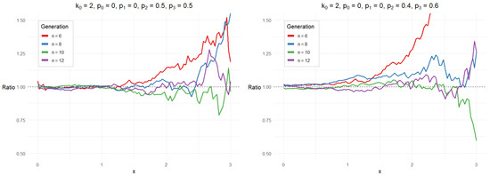
Figure 1. Ratios ${\displaystyle \frac{\mathbb{P}\left(T_n\ge x\right)}{1-\mathsf{\Phi }\left(x\right)}}$ for $n=6,8,10,12$ and $p=(0,0,0.5,0.5,0,\dots ),(0,0,0.4,0.6,0,\dots )$.

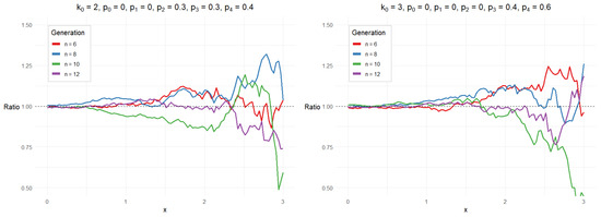
Figure 2. Ratios ${\displaystyle \frac{\mathbb{P}\left(T_n\ge x\right)}{1-\mathsf{\Phi }\left(x\right)}}$ for $n=6,8,10,12$ and $p=(0,0,0.3,0.3,0.4,0,\dots ),(0,0,0,0.4,0.6,0,\dots )$.

4. Application to Constructing Confidence Intervals of $\mathit{m}$

Assume that the offspring numbers ${\left(X_{n,i}\right)}_{1\le i\le Z_n}$ can be observed for some n. By self-normalized Cramér type moderate deviations, we have the following result for constructing confidence intervals of m.

Proposition 1.  

Assume that the conditions of Theorem 2 are satisfied. Let ${\kappa }_n\in (0,1)$ such that it holds

$$|ln{\kappa }_n|=o\left(k_0^{\frac{n\rho }{2+\rho }}\right),n\to \infty .$$

(13)

Denote

$${\Delta }_n={\displaystyle \frac{{\mathsf{\Phi }}^{-1}(1-{\kappa }_n/2)}{Z_n}}\sqrt{\sum _{i=1}^{Z_n}{(X_{n,i}-{\displaystyle \frac{Z_{n+1}}{Z_n}})}^2}.$$

(14)

Then $[A_n,B_n]$ is a 1-${\kappa }_n$ confidence interval for m as n is large enough, where

$$A_n={\displaystyle \frac{Z_{n+1}}{Z_n}}-{\Delta }_n\mathrm{and}{B}_n={\displaystyle \frac{Z_{n+1}}{Z_n}}+{\Delta }_n.$$

Proof.  

By Corollary 1, the following equalities

$${\displaystyle \frac{\mathbb{P}\left(T_n\ge x\right)}{1-\mathsf{\Phi }\left(x\right)}}=1+o\left(1\right)\mathrm{and}{\displaystyle \frac{\mathbb{P}\left(T_n\le -x\right)}{1-\mathsf{\Phi }\left(x\right)}}=1+o\left(1\right)$$

(15)

hold uniformly for $0\le x=o\left(k_0^{\frac{n\rho }{4+2\rho }}\right)$, $n\to \infty$. Denote ${\mathsf{\Phi }}^{-1}$ the inverse function of the standard normal distribution function $\mathsf{\Phi }$. Then it satisfies the following asymptotic expansion

$${\mathsf{\Phi }}^{-1}(1-p_n)=\sqrt{ln(1/p_n^2)-lnln(1/p_n^2)-ln\left(2\pi \right)}+o\left(p_n\right),p_n\searrow 0.$$

When the condition (13) is satisfied, it holds ${\mathsf{\Phi }}^{-1}(1-{\kappa }_n/2)=O(\sqrt{|ln{\kappa }_n|}$). Thus ${\mathsf{\Phi }}^{-1}(1-{\kappa }_n/2)$ is of order $o\left(k_0^{\frac{n\rho }{4+2\rho }}\right)$ as $n\to \infty$. Then, applying the last equality to (15), we obtain

$$\mathbb{P}\left(T_n\ge {\mathsf{\Phi }}^{-1}(1-{\kappa }_n/2)\right)\sim {\kappa }_n/2\mathrm{and}\mathbb{P}\left(T_n\le -{\mathsf{\Phi }}^{-1}(1-{\kappa }_n/2)\right)\sim {\kappa }_n/2,n\to \infty .$$

Clearly, the inequality $T_n\le {\mathsf{\Phi }}^{-1}(1-{\kappa }_n/2)$ is equivalent to $m\ge A_n,$ while $T_n\ge -{\mathsf{\Phi }}^{-1}(1-{\kappa }_n/2)$ is equivalent to $m\le B_n.$ Then we complete the proof of Proposition 1. □

5. Proof of Theorem 1

The proof of Theorem 1 is based on the following technical lemma of Shao [17] and the total probability formula. The total probability formula allows us to fix the population $Z_n$ such that the large deviation probabilities can be approximated by the self-normalized large deviation principle of Shao [17].

For self-normalized sums of independent random variables, Shao [17] has established the following large deviation principle.

Lemma 1.  

Let $Y,Y_1,Y_2,\dots$ be i.i.d. random variables. Assume that $\mathbb{E}Y=0$. Denote $V_n^2={\sum }_{i=1}^n{Y}_i^2$ and $S_n={\sum }_{i=1}^n{Y}_i$. Then it holds for any $x>0$,

$$\underset{n\to \infty }{lim}\mathbb{P}{\left(S_n\ge x\sqrt{n}{V}_n\right)}^{1/n}=\underset{c\ge 0}{sup}\underset{u\ge 0}{inf}\mathbb{E}\left[e^{u\left(cY-x\left(Y^2+c^2\right)/2\right)}\right].$$

(16)

In the sequel, we present the proof of Theorem 1. Denote

$$V{\left(n\right)}^2=\sum _{i=1}^{Z_n}{\left(X_{n,i}-m\right)}^2\mathrm{and}\overline{X}\left(n\right)={\displaystyle \frac{1}{Z_n}}\sum _{i=1}^{Z_n}{X}_{n,i}.$$

(17)

Let ${\left(X_i\right)}_{i\ge 1}$ be a sequence of independent random variables with the same distribution as $Z_1$. For a deterministic sample size k, denote

$$V_k^2=\sum _{i=1}^k{\left(X_i-m\right)}^2\mathrm{and}{\overline{X}}_k={\displaystyle \frac{1}{k}}\sum _{i=1}^k{X}_i.$$

(18)

Then we have $\overline{X}\left(n\right)={\displaystyle \frac{Z_{n+1}}{Z_n}}$ and

$$\sum _{i=1}^{Z_n}{\left(X_{n,i}-\overline{X}\left(n\right)\right)}^2=V{\left(n\right)}^2-Z_n{(m-\overline{X}\left(n\right))}^2.$$

(19)

When $x>0$, the probability in (3) can be reformulated as

$$\mathbb{P}\left(\left|\sum _{i=1}^{Z_n}\left(X_{n,i}-m\right)\right|\ge x\sqrt{Z_n}\sqrt{V{\left(n\right)}^2-Z_n{\left(m-\overline{X}\left(n\right)\right)}^2}\right).$$

(20)

By the assumption of the theorem, it holds $p_0=p_1=\dots =p_{k_0-1}=0$ and $0<p_{k_0}<1$, where $k_0\ge 2$. Thus, it holds $Z_n\ge k_0^n$ a.s. for any integer $n\ge 1$. Recall that $Z_n$ and ${\left(X_{n,i}\right)}_{i\ge 1}$ are independent. By the total probability formula, we obtain for any $x>0,$

$$\begin{array}{cc}& \mathbb{P}\left(\left|\sum _{i=1}^{Z_n}\left(X_{n,i}-m\right)\right|\ge x\sqrt{Z_n}\sqrt{V{\left(n\right)}^2-Z_n{\left(m-\overline{X}\left(n\right)\right)}^2}\right)\hfill \\ & =\sum _{t=k_0^n}^{\infty }\mathbb{P}\left(\left|\sum _{i=1}^t\left(X_i-m\right)\right|\ge x\sqrt{t}\sqrt{V_t^2-t{\left(m-\overline{X}\right)}^2},Z_n=t\right)\hfill \\ & =\sum _{t=k_0^n}^{\infty }\mathbb{P}\left(Z_n=t\right)\mathbb{P}\left(\left|\sum _{i=1}^t\left(X_i-m\right)\right|\ge x\sqrt{t}\sqrt{V_t^2-t{\left(m-\overline{X}\right)}^2}\right)\hfill \\ & :=\sum _{t=k_0^n}^{\infty }\mathbb{P}\left(Z_n=t\right)\psi \left(t,x\right).\hfill \end{array}$$

Now, we divide the term $\psi \left(t,x\right)$ into two parts

$$\begin{array}{cc}\hfill \psi (t,x)& =\mathbb{P}\left(\sum _{i=1}^t(X_i-m)\ge x\sqrt{t}\sqrt{V_t^2-t{(m-{\overline{X}}_t)}^2}\right)\hfill \\ \hfill & +\mathbb{P}\left(\sum _{i=1}^t(m-X_i)\ge x\sqrt{t}\sqrt{V_t^2-t{(m-{\overline{X}}_t)}^2}\right)\hfill \\ \hfill & :=I\left(t\right)+J\left(t\right).\hfill \end{array}$$

For $I\left(t\right)$, we have the following estimation

$$\begin{array}{cc}\hfill I\left(t\right)& =\mathbb{P}\left(\sum _{i=1}^t(X_i-m)\ge x\sqrt{t}\sqrt{V_t^2-t{(m-{\overline{X}}_k)}^2},t{\left(m-{\overline{X}}_t\right)}^2<{\displaystyle \frac{1}{4}}{V}_t^2\right)\hfill \\ \hfill & +\mathbb{P}\left(\sum _{i=1}^t(X_i-m)\ge x\sqrt{t}\sqrt{V_t^2-t{(m-{\overline{X}}_k)}^2},t{\left(m-{\overline{X}}_t\right)}^2\ge {\displaystyle \frac{1}{4}}{V}_t^2\right)\hfill \\ \hfill & \le \mathbb{P}\left(\sum _{i=1}^t(X_i-m)\ge x\sqrt{{\displaystyle \frac{3}{4}}t}{V}_t\right)+\mathbb{P}\left(t{(m-{\overline{X}}_t)}^2\ge {\displaystyle \frac{1}{4}}{V}_t^2\right).\hfill \end{array}$$

(21)

Note that

$$t{(m-{\overline{X}}_t)}^2={\displaystyle \frac{1}{t}}{\left(\sum _{i=1}^t(X_i-m)\right)}^2.$$

Thus, the second term in (21) can be reformulated as

$$\begin{array}{cc}\hfill \mathbb{P}\left(t{(m-{\overline{X}}_t)}^2\ge {\displaystyle \frac{1}{4}}{V}_t^2\right)& =\mathbb{P}\left({\left(\sum _{i=1}^t(X_i-m)\right)}^2\ge {\displaystyle \frac{1}{4}}t{V}_t^2\right)\hfill \\ \hfill & =\mathbb{P}\left(\sum _{i=1}^t\left(X_i-m\right)\ge {\displaystyle \frac{1}{2}}\sqrt{t}{V}_t\right)+\mathbb{P}\left(\sum _{i=1}^t\left(m-X_i\right)\ge {\displaystyle \frac{1}{2}}\sqrt{t}{V}_t\right).\hfill \end{array}$$

(22)

According to Lemma 1 with centered variables $Y_i=X_i-m$, for any small positive $\delta$, it holds for all the integers t to be large enough,

$$\begin{array}{c}\hfill \mathbb{P}\left(\sum _{i=1}^t\left(X_i-m\right)\ge {\displaystyle \frac{1}{2}}\sqrt{t}{V}_t\right)\le {(1+\delta )}^t{\rho }_1^t,\end{array}$$

(23)

where

$$\begin{array}{c}\hfill {\rho }_1:=\underset{c\ge 0}{sup}\underset{u\ge 0}{inf}\mathbb{E}\left[exp\left\{u\left(c(X-m)-{\displaystyle \frac{1}{2}}\left({(X-m)}^2+c^2\right)/2\right)\right\}\right]\in (0,1).\end{array}$$

Similarly, for the second term on the right-hand side of (22), it holds for all integers t to be large enough,

$$\mathbb{P}\left(\sum _{i=1}^t\left(m-X_i\right)\ge {\displaystyle \frac{1}{2}}\sqrt{t}{V}_t\right)\le {(1+\delta )}^t{\rho }_2^t,$$

(24)

where

$$\begin{array}{c}\hfill {\rho }_2:=\underset{c\ge 0}{sup}\underset{u\ge 0}{inf}\mathbb{E}\left[exp\left\{u\left(c(m-X)-{\displaystyle \frac{1}{2}}\left({(m-X)}^2+c^2\right)/2\right)\right\}\right]\in (0,1).\end{array}$$

Similarly, for any $x>0$, we can deduce that for any positive $\delta \left(x\right)$ and all integers t to be large enough,

$$\begin{array}{cc}\hfill \mathbb{P}\left(\sum _{i=1}^t\left(X_i-m\right)\ge x\sqrt{{\displaystyle \frac{3}{4}}t}{V}_t\right)& \le {\left(1+\delta \left(x\right)\right)}^t{\rho }_3^t\left(x\right),\hfill \end{array}$$

(25)

where

$$\begin{array}{c}\hfill {\rho }_3\left(x\right):=\underset{c\ge 0}{sup}\underset{u\ge 0}{inf}\mathbb{E}\left[exp\left\{u\left(c(X-m)-x\sqrt{{\displaystyle \frac{3}{4}}}\left({(X-m)}^2+c^2\right)/2\right)\right\}\right]\in (0,1).\end{array}$$

By an argument similar to the estimation of $J\left(t\right)$, we can deduce that for any positive $\delta \left(x\right),x>0,$ it holds for all integers t to be large enough,

$$\begin{array}{c}\hfill J\left(t\right)\le 3{(1+\delta \left(x\right))}^t{\rho }_4^t\left(x\right)\end{array}$$

(26)

with some ${\rho }_4\left(x\right)\in (0,1)$. Now we define $\rho \left(x\right)=max\left\{{\rho }_1,{\rho }_2,{\rho }_3\left(x\right),{\rho }_4\left(x\right)\right\}$ and choose a $\delta \left(x\right)\in (0,1)$ such that $(1+\delta \left(x\right))\rho \left(x\right)<1$. Therefore, by (21)–(26), we can deduce that for any $x>0$ and all the n to be large enough,

$$\begin{array}{c}\hfill \psi (t,x)=I\left(t\right)+J\left(t\right)\le 6{(1+\delta \left(x\right))}^t{\rho }^t\left(x\right)\le 6{(1+\delta \left(x\right))}^{k_0^n}{\rho }^{k_0^n}\left(x\right).\end{array}$$

Thus, when $n\to \infty$, the probability (20) can be rewritten as follows: For any $x>0,$

$$\begin{array}{cc}& \mathbb{P}\left(\left|\sum _{i=1}^{Z_n}\left(X_{n,i}-m\right)\right|\ge x\sqrt{Z_n}\sqrt{V{\left(n\right)}^2-Z_n{\left(m-\overline{X}\left(n\right)\right)}^2}\right)\hfill \\ & =\sum _{t=k_0^n}^{\infty }\mathbb{P}\left(Z_n=t\right)\psi \left(t,x\right)\hfill \\ & \le 6{(1+\delta \left(x\right))}^{k_0^n}{\rho }^{k_0^n}\left(x\right)\sum _{t=k_0^n}^{\infty }\mathbb{P}(Z_n=t)\hfill \\ & =6{(1+\delta \left(x\right))}^{k_0^n}{\rho }^{k_0^n}\left(x\right).\hfill \end{array}$$

By taking logarithms of both sides, we can deduce that for any $x>0,$

$$\underset{n\to \infty }{lim\; sup}{\displaystyle \frac{1}{k_0^n}}ln\mathbb{P}\left({\displaystyle \frac{\sqrt{Z_n}}{\sqrt{{\sum }_{i=1}^{Z_n}{\left(X_{n,i}-\frac{Z_{n+1}}{Z_n}\right)}^2}}}\left|{\displaystyle \frac{Z_{n+1}}{Z_n}}-m\right|\ge x\right)\le -\lambda \left(x\right),$$

where $\lambda \left(x\right)=-ln\left[(1+\delta \left(x\right))\rho \left(x\right)\right]>0$. This completes the proof of Theorem 1.

6. Proof of Theorem 2

The proof of Theorem 2 is based on the following technical lemma of Jing et al. [15] and the total probability formula. For self-normalized sums of independent random variables, Jing et al. [15] have established the following self-normalized Cramér moderate deviation.

Lemma 2.  

Let ${\left(Y_i\right)}_{i\ge 1}$ be a sequence of i.i.d. and centered random variables. Assume there exists a constant $\rho \in (0,1]$ such that $\mathbb{E}{Y}_1^{2+\rho }<\infty$. Denote $S_n={\sum }_{i=1}^n{Y}_i$ and $V_n^2={\sum }_{i=1}^n{Y}_i^2$. Then it holds

$$\left|ln{\displaystyle \frac{\mathbb{P}\left(S_n/V_n\ge x\right)}{1-\mathsf{\Phi }\left(x\right)}}\right|\le C{\displaystyle \frac{1+x^{2+\rho }}{n^{\rho /2}}}$$

(27)

uniformly for $0\le x=o\left(\sqrt{n}\right)$, $n\to \infty$.

Recall that $Z_n$ is the number of individuals in the n-th generation, and $X_{n,i}$, $1\le i\le Z_n$, is the offspring number of the i-th individual in the n-th generation. Denote

$$V{\left(n\right)}^2=\sum _{i=1}^{Z_n}{\left(X_{n,i}-m\right)}^2,V_k^2=\sum _{i=1}^k{\left(X_{n,i}-m\right)}^2,\overline{X}\left(n\right)={\displaystyle \frac{Z_{n+1}}{Z_n}},{\overline{Y}}_n={\displaystyle \frac{Z_{n+1}}{n}}.$$

(28)

Then it holds

$$\begin{array}{cc}\hfill \sum _{i=1}^{Z_n}{\left(X_{n,i}-\overline{X}\left(n\right)\right)}^2& =\sum _{i=1}^{Z_n}\left(\left(X_{n,i}-m\right)+(m-\overline{X}\left(n\right)){)}^2\right.\hfill \\ \hfill & =V{\left(n\right)}^2-Z_n{(m-\overline{X}\left(n\right))}^2.\hfill \end{array}$$

(29)

Therefore, we can rewrite $T_n$ as follows

$$T_n={\displaystyle \frac{{\sum }_{i=1}^{Z_n}\left(X_{n,i}-m\right)}{\sqrt{V{\left(n\right)}^2-Z_n{(m-\overline{X}\left(n\right))}^2}}}.$$

(30)

Recall that $Z_n$ and ${\left(X_{n,i}\right)}_{i\ge 1}$ are independent. By the law of total probability, we can deduce that for any $x\ge 0$,

$$\begin{array}{ccc}\hfill \mathbb{P}\left(T_n\ge x\right)& =& \mathbb{P}\left(\sum _{i=1}^{Z_n}\left(X_{n,i}-m\right)\ge x\sqrt{V{\left(n\right)}^2-Z_n{(m-\overline{X}\left(n\right))}^2}\right)\hfill \\ & =& \sum _{t=k_0^n}^{\infty }\mathbb{P}\left(\sum _{i=1}^{Z_n}\left(X_{n,i}-m\right)\ge x\sqrt{V{\left(n\right)}^2-Z_n{(m-\overline{X}\left(n\right))}^2},Z_n=t\right)\hfill \\ & =& \sum _{t=k_0^n}^{\infty }\mathbb{P}\left(Z_n=t\right)\mathbb{P}\left(\sum _{i=1}^t\left(X_{n,i}-m\right)\ge x\sqrt{V_t^2-t{\left(m-{\overline{Y}}_t\right)}^2}\right)\hfill \\ & =& \sum _{t=k_0^n}^{\infty }\mathbb{P}\left(Z_n=t\right)\mathbb{P}\left(\sum _{i=1}^t\left(X_{n,i}-m\right)\ge x\sqrt{V_t^2-t{\left(m-{\overline{Y}}_t\right)}^2}\right)\hfill \\ & =& \sum _{t=k_0^n}^{\infty }\mathbb{P}\left(Z_n=t\right)I_t\left(x\right).\hfill \end{array}$$

(31)

For any integer $t\ge k_0^n$, it is easy to see that for all $x\ge 0$,

$$\begin{array}{cc}\hfill I_t\left(x\right)& =\mathbb{P}\left(\sum _{i=1}^t\left(X_{n,i}-m\right)\ge x\sqrt{V_t^2-t{\left(m-{\overline{Y}}_t\right)}^2},t{\left(m-{\overline{Y}}_t\right)}^2<V_t^2(1+x^{\rho })/t^{\rho /2}\right)\hfill \\ & +\mathbb{P}\left(\sum _{i=1}^t\left(X_{n,i}-m\right)\ge x\sqrt{V_t^2-t{\left(m-{\overline{Y}}_t\right)}^2},t{\left(m-{\overline{Y}}_t\right)}^2\ge V_t^2(1+x^{\rho })/t^{\rho /2}\right)\hfill \\ \hfill & \le \mathbb{P}\left(\sum _{i=1}^t\left(X_{n,i}-m\right)\ge x{V}_t\sqrt{1-(1+x^{\rho })/t^{\rho /2}}\right)+\mathbb{P}\left(t{\left(m-{\overline{Y}}_t\right)}^2\ge V_t^2(1+x^{\rho })/t^{\rho /2}\right)\hfill \\ \hfill & =:I_{t,1}\left(x\right)+I_{t,2}\left(x\right).\hfill \end{array}$$

We first give an estimation for $I_{t,1}\left(x\right)$. Recall that ${(X_{n,i}-m)}_{i\ge 1}$ are independent of $Z_n$. When $t\ge k_0^n$, by Lemma 2, we obtain for all $0\le x=o\left(k_0^{\frac{n}{2}}\right)$,

$$\left|ln{\displaystyle \frac{I_{t,1}\left(x\right)}{1-\mathsf{\Phi }\left(x\sqrt{1-(1+x^{\rho })/t^{\rho /2}}\right)}}\right|\le C_2{\displaystyle \frac{1+x^{2+\rho }}{t^{\rho /2}}}\le C_2{\displaystyle \frac{1+x^{2+\rho }}{k_0^{n\rho /2}}}.$$

Using the inequalities

$${\displaystyle \frac{1}{\sqrt{2\pi }(1+x)}}{e}^{-x^2/2}\le 1-\mathsf{\Phi }\left(x\right)\le {\displaystyle \frac{1}{\sqrt{\pi }(1+x)}}{e}^{-x^2/2},x\ge 0,$$

(32)

we can deduce that for all $x\ge 0$ and $0\le \epsilon \le 1$,

$$\begin{array}{cc}\hfill {\displaystyle \frac{1-\mathsf{\Phi }\left(x\sqrt{1-\epsilon }\right)}{1-\mathsf{\Phi }\left(x\right)}}& =1+{\displaystyle \frac{{\int }_{x\sqrt{1-\epsilon }}^x\frac{1}{\sqrt{2\pi }}{e}^{-s^2/2}ds}{1-\mathsf{\Phi }\left(x\right)}}\le 1+{\displaystyle \frac{\frac{1}{\sqrt{2\pi }}{e}^{-x^2(1-\epsilon )/2}x\epsilon }{\frac{1}{\sqrt{2\pi }(1+x)}{e}^{-x^2/2}}}\hfill \\ \hfill & \le 1+C(1+x^2)\epsilon e^{x^2\epsilon /2}\hfill \\ \hfill & \le exp\left\{C(1+x^2)\epsilon \right\}.\hfill \end{array}$$

(33)

Using the last inequality, we deduce that for all $t\ge k_0^n$ and all $0\le x=o\left(k_0^{\frac{n}{2}}\right)$,

$$\begin{array}{cc}\hfill I_{t,1}\left(x\right)& \le \left(1-\mathsf{\Phi }\left(x\sqrt{1-(1+x^{\rho })/t^{\rho /2}}\right)\right)exp\left\{C_2{\displaystyle \frac{1+x^{2+\rho }}{k_0^{n\rho /2}}}\right\}\hfill \\ \hfill & \le \left(1-\mathsf{\Phi }\left(x\right)\right)exp\left\{C_2{\displaystyle \frac{1+x^{2+\rho }}{k_0^{n\rho /2}}}+C(1+x^2){\displaystyle \frac{1+x^{\rho }}{t^{\rho /2}}}\right\}\hfill \\ \hfill & \le \left(1-\mathsf{\Phi }\left(x\right)\right)exp\left\{C_3{\displaystyle \frac{1+x^{2+\rho }}{k_0^{n\rho /2}}}\right\},\hfill \end{array}$$

(34)

which gives an estimation of $I_{t,1}\left(x\right)$.

Next, we consider the estimation of $I_{t,2}\left(x\right)$. Notice that

$$t{\left(m-{\overline{Y}}_t\right)}^2={\displaystyle \frac{1}{t}}{\left(\sum _{i=1}^t\left(X_{n,i}-m\right)\right)}^2.$$

Then we have

$$\begin{array}{cc}\hfill I_{t,2}\left(x\right)& =\mathbb{P}\left({\left(\sum _{i=1}^t\left(X_{n,i}-m\right)\right)}^2\ge t^{1-\rho /2}{V}_t^2(1+x^{\rho })\right)\hfill \\ & =\mathbb{P}\left(\left|\sum _{i=1}^t\left(X_{n,i}-m\right)\right|\ge V_t\sqrt{t^{1-\rho /2}(1+x^{\rho })}\right).\hfill \end{array}$$

Applying Lemma 2 to the centered random variables ${(\pm (X_{n,i}-m))}_{i\ge 1},$ we deduce that for all $t\ge k_0^n$ and all $0\le x=o\left(k_0^{n/2}\right)$,

$$\begin{array}{cc}\hfill I_{t,2}\left(x\right)& \le 2\left(1-\mathsf{\Phi }\left(\sqrt{t^{1-\rho /2}(1+x^{\rho })}\right)\right)exp\left\{C{\displaystyle \frac{1+(\sqrt{t^{1-\rho /2}(1+x^{\rho })}{)}^{2+\rho }}{\sqrt{t}}}\right\}\hfill \\ \hfill & \le 2exp\left\{-{\displaystyle \frac{1}{4}}{t}^{1-\rho /2}(1+x^{\rho })\right\},\hfill \end{array}$$

where the last inequality follows by (32). Again by (32), we obtain for all $t\ge k_0^n$ and all $0\le x=o\left(k_0^{n/2}\right)$,

$$\begin{array}{cc}\hfill I_{t,2}\left(x\right)& \le 2exp\left\{-{\displaystyle \frac{1}{4}}{k}_0^{n-n\rho /2}(1+x^{\rho })\right\}\hfill \\ \hfill & \le C{\displaystyle \frac{1+x}{k_0^n}}\left(1-\mathsf{\Phi }\left(x\right)\right),\hfill \end{array}$$

(35)

which gives an estimation of $I_{t,2}\left(x\right)$.

Combining (32), (34) and (35) together, we obtain for all $t\ge k_0^n$ and all $0\le x=o\left(k_0^{n/2}\right)$,

$$I_t\left(x\right)\le \left(1-\mathsf{\Phi }\left(x\right)\right)exp\left\{C_4{\displaystyle \frac{1+x^{2+\rho }}{k_0^{n\rho /2}}}\right\}.$$

(36)

Returning to (31), by the last inequality, we deduce that for all $0\le x=o\left(k_0^{n/2}\right)$,

$$\begin{array}{cc}\hfill \mathbb{P}\left(T_n\ge x\right)& =\sum _{t=k_0^n}^{\infty }\mathbb{P}\left(Z_n=t\right)I_t\left(x\right)\hfill \\ \hfill & \le \sum _{t=k_0^n}^{\infty }\mathbb{P}\left(Z_n=t\right)\left(1-\mathsf{\Phi }\left(x\right)\right)exp\left\{C_4{\displaystyle \frac{1+x^{2+\rho }}{k_0^{n\rho /2}}}\right\}\hfill \\ \hfill & =\left(1-\mathsf{\Phi }\left(x\right)\right)exp\left\{C_4{\displaystyle \frac{1+x^{2+\rho }}{k_0^{n\rho /2}}}\right\}.\hfill \end{array}$$

(37)

Next, we give an estimation for the lower bound of $\mathbb{P}\left(T_n\ge x\right)$. For $I_t\left(x\right)$, it is easy to see that for all $t\ge k_0^n$ and all $0\le x=o\left(k_0^{\frac{n}{2}}\right)$,

$$\begin{array}{cc}\hfill I_t\left(x\right)& =\mathbb{P}\left(\sum _{i=1}^t\left(X_{n,i}-m\right)\ge x\sqrt{V_t^2-t{(m-{\overline{Y}}_t)}^2}\right)\hfill \\ \hfill & \ge \mathbb{P}\left(\sum _{i=1}^t\left(X_{n,i}-m\right)\ge x{V}_t\right).\hfill \end{array}$$

When $t\ge k_0^n$, by Lemma 2, we obtain for all $0\le x=o\left(k_0^{\frac{n}{2}}\right)$,

$$\begin{array}{c}\hfill I_t\left(x\right)\ge \left(1-\mathsf{\Phi }\left(x\right)\right)exp\left\{-C_5{\displaystyle \frac{1+x^{2+\rho }}{k_0^{n\rho /2}}}\right\}.\end{array}$$

Returning to (31), we obtain for all $0\le x=o\left(k_0^{n/2}\right)$,

$$\begin{array}{cc}\hfill \mathbb{P}\left(T_n\ge x\right)& =\sum _{t=k_0^n}^{\infty }\mathbb{P}\left(Z_n=t\right)I_t\left(x\right)\hfill \\ \hfill & \ge \left(1-\mathsf{\Phi }\left(x\right)\right)exp\left\{-C_5{\displaystyle \frac{1+x^{2+\rho }}{k_0^{n\rho /2}}}\right\}.\hfill \end{array}$$

(38)

Combining (37) and (38) together, we obtain the desired inequality.

The same argument holds for ${\left(m-X_{n,k}\right)}_{k\ge 1}$. Therefore, the first equality also holds when ${\displaystyle \frac{\mathbb{P}(T_n\ge x)}{1-\mathsf{\Phi }\left(x\right)}}$ is replaced by ${\displaystyle \frac{\mathbb{P}(T_n\le -x)}{\mathsf{\Phi }(-x)}}$. Then we complete the proof of Theorem 2.

7. Proof of Corollary 2

Firstly, we show that it holds for any Borel set B,

$$\underset{n\to \infty }{lim\; sup}{\displaystyle \frac{1}{a^2}}ln\left({\displaystyle \frac{T_n}{a_n}}\in B\right)\le -\underset{x\in \overline{B}}{inf}{\displaystyle \frac{x^2}{2}}.$$

(39)

Indeed, when $B=\varnothing$, the equality (39) holds obviously. When $B\ne \varnothing$, for $\rho \in \left(0,1\right]$ and $a_n=o\left(k_0^{n/2}\right)$, define $x_0=\underset{x\in B}{inf}\left|x\right|$. Then, by Theorem 2, we obtain

$$\mathbb{P}\left({\displaystyle \frac{T_n}{a_n}}\in B\right)\le \mathbb{P}\left(|T_n| \ge a_n{x}_0\right)\le 2\left(1-\mathsf{\Phi }\left(a_n{x}_0\right)\right)exp\left\{C{\displaystyle \frac{1+x^{2+\rho }}{k_0^{n\rho /2}}}\right\}.$$

(40)

Notice the fact that $a_n\to \infty$ and $a_n/\sqrt{k_0^n}\to 0$. Combining the above inequality with (32), we obtain

$$\begin{array}{c}\hfill \underset{n\to \infty }{lim\; sup}{\displaystyle \frac{1}{a_n^2}}ln\mathbb{P}\left({\displaystyle \frac{T_n}{a_n}}\in B\right)\le \underset{n\to \infty }{lim}{\displaystyle \frac{1}{a_n^2}}\left(-{\displaystyle \frac{{\left(a_n{x}_0\right)}^2}{2}}-ln\left(a_n{x}_0\right)\right).\end{array}$$

(41)

Notice that ${\displaystyle \frac{1}{a_n^2}}ln\left(a_n{x}_0\right)\to 0$ when $n\to \infty$, then

$$\underset{n\to \infty }{lim\; sup}{\displaystyle \frac{1}{a_n^2}}ln\mathbb{P}\left({\displaystyle \frac{T_n}{a_n}}\in B\right)\le -{\displaystyle \frac{{x_0}^2}{2}}\le -\underset{x\in \overline{B}}{inf}{\displaystyle \frac{x^2}{2}},$$

(42)

which gives (39).

Next, we show that the following lower bound holds

$$\underset{n\to \infty }{lim\; inf}{\displaystyle \frac{1}{a_n^2}}ln\mathbb{P}\left({\displaystyle \frac{T_n}{a_n}}\in B\right)\ge -\underset{x\in \mathring{B}}{inf}{\displaystyle \frac{x^2}{2}}.$$

(43)

When $\mathring{B}=\varnothing$, the last inequality holds obviously. When $\mathring{B}\ne \varnothing$, as $\mathring{B}$ is an open set, for any ${\epsilon }_1>0$ small enough, we can find an $x_0\in \mathring{B}$ such that the following inequalities hold

$$0<{\displaystyle \frac{{x_0}^2}{2}}\le \underset{x\in \mathring{B}}{inf}{\displaystyle \frac{x^2}{2}}+{\epsilon }_1.$$

(44)

Since $\mathring{B}$ is an open set, for $x_0\in \mathring{B}$ and some small ${\epsilon }_2\in \left(0,\left|x_0\right|\right]$, we have $\left(x_0-{\epsilon }_2,x_0+{\epsilon }_2\right]\subset \mathring{B}$. Then,

$$\begin{array}{cc}\hfill \mathbb{P}\left({\displaystyle \frac{T_n}{a_n}}\in B\right)& \ge \mathbb{P}\left(T_n\in \left(a_n\left(x_0-{\epsilon }_2\right),a_n\left(x_0+{\epsilon }_2\right)\right]\right)\hfill \\ & =\mathbb{P}\left(T_n>a_n\left(x_0-{\epsilon }_2\right)\right)-\mathbb{P}\left(T_n>a_n\left(x_0+{\epsilon }_2\right)\right).\hfill \end{array}$$

(45)

By Theorem 2, we can deduce that when $a_n\to \infty$ and $a_n/\sqrt{k_0^n}\to 0$, it holds

$$\underset{n\to \infty }{lim}{\displaystyle \frac{\mathbb{P}\left(T_n>a_n\left(x_0+{\epsilon }_2\right)\right)}{\mathbb{P}\left(T_n>a_n\left(x_0-{\epsilon }_2\right)\right)}}=0.$$

(46)

By (32) and the last equality, we deduce that there exists a large number N such that for all $n>N$,

$$\begin{array}{cc}\hfill \mathbb{P}\left({\displaystyle \frac{T_n}{a_n}}\in B\right)& \ge \mathbb{P}\left(T_n\ge a_n\left(x_0-{\epsilon }_2\right)\right)-{\displaystyle \frac{1}{4}}\mathbb{P}\left(T_n\ge a_n\left(x_0-{\epsilon }_2\right)\right)\hfill \\ & ={\displaystyle \frac{3}{4}}\mathbb{P}\left(T_n\ge a_n\left(x_0-{\epsilon }_2\right)\right)\hfill \\ & \ge {\displaystyle \frac{3}{4}}\left(1-\mathsf{\Phi }\left(a_n\left(x_0-{\epsilon }_2\right)\right)\right)exp\left\{-C{\displaystyle \frac{1+{a_n}^{2+\rho }{\left(x_o-{\epsilon }_2\right)}^{2+\rho }}{k_0^{n\rho /2}}}\right\}\hfill \\ & \ge {\displaystyle \frac{3/4}{\sqrt{2\pi }(1+a_n\left(x_0-{\epsilon }_2\right))}}exp\left\{-{\displaystyle \frac{1}{2}}{a_n}^2{\left(x_0-{\epsilon }_2\right)}^2-C{\displaystyle \frac{1+{a_n}^{2+\rho }{\left(x_o-{\epsilon }_2\right)}^{2+\rho }}{k_0^{n\rho /2}}}\right\},\hfill \end{array}$$

which implies that

$$\begin{array}{cc}\hfill \underset{n\to \infty }{lim\; inf}{\displaystyle \frac{1}{a_n^2}}ln\mathbb{P}\left({\displaystyle \frac{T_n}{a_n}}\in B\right)& \ge -{\displaystyle \frac{1}{2}}{\left(x_0-{\epsilon }_2\right)}^2\ge -\underset{x\in \mathring{B}}{inf}{\displaystyle \frac{x^2}{2}}-{\epsilon }_1.\hfill \end{array}$$

(47)

Letting ${\epsilon }_1\to 0$, we obtain (43). Combining inequalities (39) and (43) together, we obtain the desired result.

8. Proof of Corollary 3

It is obvious that

$$\begin{array}{cc}\hfill & \underset{x\in R}{sup}|\mathbb{P}\left(T_n\le x\right)-\mathsf{\Phi }\left(x\right)|\hfill \\ \hfill & \le \underset{x\ge k_0^{n\rho /\left(9+4\rho \right)}}{sup}|\mathbb{P}\left(T_n\le x\right)-\mathsf{\Phi }\left(x\right)|+\underset{0\le x<k_0^{n\rho /\left(9+4\rho \right)}}{sup}|\mathbb{P}\left(T_n\le x\right)-\mathsf{\Phi }\left(x\right)|\hfill \\ & +\underset{-k_0^{n\rho /\left(9+4\rho \right)}<x\le 0}{sup}|\mathbb{P}\left(T_n\le x\right)-\mathsf{\Phi }\left(x\right)|+\underset{x\le -k_0^{n\rho /\left(9+4\rho \right)}}{sup}|\mathbb{P}\left(T_n\le x\right)-\mathsf{\Phi }\left(x\right)|\hfill \\ & =:H_1+H_2+H_3+H_4.\hfill \end{array}$$

(48)

By Theorem 2 and (32), we can deduce that

$$\begin{array}{cc}\hfill H_1& =\underset{x\ge k_0^{n\rho /\left(9+4\rho \right)}}{sup}\left|\mathbb{P}\left(T_n>x\right)-\left(1-\mathsf{\Phi }\left(x\right)\right)\right|\hfill \\ & \le \underset{x\ge k_0^{n\rho /\left(9+4\rho \right)}}{sup}\mathbb{P}\left(T_n>x\right)+\underset{x\ge k_0^{n\rho /\left(9+4\rho \right)}}{sup}\left(1-\mathsf{\Phi }\left(x\right)\right)\hfill \\ & \le \mathbb{P}\left(T_n\ge k_0^{n\rho /\left(9+4\rho \right)}\right)+\left(1-\mathsf{\Phi }\left(k_0^{n\rho /\left(9+4\rho \right)}\right)\right)\hfill \\ & \le \left(1-\mathsf{\Phi }\left(k_0^{n\rho /\left(9+4\rho \right)}\right)\right)e^c+exp\left\{-{\displaystyle \frac{1}{2}}{\left(k_0^{n\rho /\left(9+4\rho \right)}\right)}^2\right\}\hfill \\ & \le {\displaystyle \frac{C_1}{k_0^{n\rho /2}}}\hfill \end{array}$$

(49)

and

$$\begin{array}{cc}\hfill H_4& \le \underset{x\le -k_0^{n\rho /\left(9+4\rho \right)}}{sup}\mathbb{P}\left(T_n\le x\right)+\underset{x\le -k_0^{n\rho /\left(9+4\rho \right)}}{sup}\mathsf{\Phi }\left(x\right)\hfill \\ & \le \mathbb{P}\left(T_n\le -k_0^{n\rho /\left(9+4\rho \right)}\right)+\mathsf{\Phi }\left(-k_0^{n\rho /\left(9+4\rho \right)}\right)\hfill \\ & \le \mathsf{\Phi }\left(-k_0^{n\rho /\left(9+4\rho \right)}\right)e^c+exp\left\{-{\displaystyle \frac{1}{2}}{\left(k_0^{n\rho /\left(9+4\rho \right)}\right)}^2\right\}\hfill \\ & \le {\displaystyle \frac{C_2}{k_0^{n\rho /2}}}.\hfill \end{array}$$

(50)

Then by Theorem 2, using the inequality $\left|e^x-1\right|\le \left|x\right|e^{\left|x\right|}$, we deduce that

$$\begin{array}{cc}\hfill H_2& =\underset{0\le x<k_0^{n\rho /\left(9+4\rho \right)}}{sup}|\mathbb{P}\left(T_n\le x\right)-\left(1-\mathsf{\Phi }\left(x\right)\right)|\hfill \\ & \le \underset{0\le x<k_0^{n\rho /\left(9+4\rho \right)}}{sup}\left(1-\mathsf{\Phi }\left(x\right)\right)\left|e^{C\left(1+x^{2+\rho }\right)/k_0^{n\rho /2}}-1\right|\hfill \\ & \le {\displaystyle \frac{C}{k_0^{n\rho /2}}}\underset{0\le x<k_0^{n\rho /\left(9+4\rho \right)}}{sup}\left(1-\mathsf{\Phi }\left(x\right)\right)\left(1+x^{2+\rho }\right)e^{C\left(1+x^{2+\rho }\right)/k_0^{n\rho /2}}\hfill \\ & \le {\displaystyle \frac{C_3}{k_0^{n\rho /2}}}\hfill \end{array}$$

(51)

and, similarly,

$$\begin{array}{cc}\hfill H_3& =\underset{-k_0^{n/9}<x\le 0}{sup}\left|\mathbb{P}\left(T_n\le x\right)-\mathsf{\Phi }\left(x\right)\right|\hfill \\ & \le \underset{-k_0^{n/9}<x\le 0}{sup}\mathsf{\Phi }\left(x\right)\left|e^{C\left(1+{\left|x\right|}^{2+\rho }\right)/k_0^{n\rho /2}}-1\right|\hfill \\ & \le {\displaystyle \frac{C_4}{k_0^{n\rho /2}}}.\hfill \end{array}$$

(52)

Combining (49)–(52) together, we obtain the desired inequality. This completes the proof of Corollary 3.

References

- Lotka, A. Theorie analytique des assiciation biologiques. Actualités Sci. Ind. 1939, 780, 123–136. [Google Scholar]
- Nagaev, S.V. On estimating the expected number of direct descendants of a particle in a branching process. Theory Probab. Appl. 1967, 12, 314–320. [Google Scholar] [CrossRef]
- Athreya, K.B. Large deviation rates for branching processes. I. Single type case. Ann. Appl. Probab. 1994, 4, 779–790. [Google Scholar] [CrossRef]
- Ney, P.E.; Vidyashankar, A.N. Harmonic moments and large deviation rates for supercritical branching processes. Ann. Appl. Probab. 2003, 13, 475–489. [Google Scholar] [CrossRef]
- Ney, P.E.; Vidyashankar, A.N. Local limit theory and large deviations for supercritical branching processes. Ann. Appl. Probab. 2004, 14, 1135–1166. [Google Scholar] [CrossRef]
- He, H. On large deviation rates for sums associated with Galton-Watson processes. Adv. Appl. Probab. 2016, 48, 672–690. [Google Scholar] [CrossRef]
- Bercu, B.; Touati, A. Exponential inequalities for self-normalized martingales with applications. Ann. Appl. Probab. 2008, 18, 1848–1869. [Google Scholar] [CrossRef]
- Chu, W. Self-normalized large deviation for supercritical branching processes. J. Appl. Probab. 2018, 55, 450–458. [Google Scholar] [CrossRef]
- Fan, X.; Shao, Q.M. Self-normalized Cramér moderate deviations for a supercritical Galton-Watson process. J. Appl. Probab. 2023, 60, 1281–1292. [Google Scholar] [CrossRef]
- Fan, X.; Shao, Q.M. Self-normalized Cramér type moderate deviations for martingales and applications. Bernoulli 2025, 31, 130–161. [Google Scholar] [CrossRef]
- Doukhan, P.; Fan, X.; Gao, Z.Q. Cramér moderate deviations for a supercritical Galton-Watson process. Statist. Probab. Letters 2023, 192, 109711. [Google Scholar] [CrossRef]
- Petrov, V.V. Sums of Independent Random Variables; Springer: Berlin, Germany, 1975. [Google Scholar]
- Beknazaryan, A.; Sang, H.; Xiao, Y. Cramér type moderate deviations for random fields. J. Appl. Probab. 2019, 56, 223–245. [Google Scholar] [CrossRef]
- Fan, X.; Shao, Q.M. Cramér’s moderate deviations for martingales with applications. Ann. Inst. H. Poincaré Probab. Statist. 2024, 60, 2046–2074. [Google Scholar] [CrossRef]
- Jing, B.Y.; Shao, Q.M.; Wang, Q. Self-normalized Cramér-type large deviations for independent random variables. Ann. Probab. 2003, 31, 2167–2215. [Google Scholar] [CrossRef]
- Fan, X.; Hu, H.; Xu, L. Normalized and self-normalized Cramér-type moderate deviations for Euler-Maruyama scheme for SDE. Sci. China Math. 2024, 67, 1865–1880. [Google Scholar] [CrossRef]
- Shao, Q.M. Self-normalized large deviations. Ann. Probab. 1997, 25, 285–328. [Google Scholar] [CrossRef]
Disclaimer/Publisher’s Note: The statements, opinions and data contained in all publications are solely those of the individual author(s) and contributor(s) and not of MDPI and/or the editor(s). MDPI and/or the editor(s) disclaim responsibility for any injury to people or property resulting from any ideas, methods, instructions or products referred to in the content. |
© 2025 by the authors. Licensee MDPI, Basel, Switzerland. This article is an open access article distributed under the terms and conditions of the Creative Commons Attribution (CC BY) license (https://creativecommons.org/licenses/by/4.0/).