Article

A Cubic Spline Numerical Method for a Singularly Perturbed Two-Parameter Ordinary Differential Equation

by
Hassan J. Al Salman
1,*,
Fasika Wondimu Gelu
2,* and
Ahmed A. Al Ghafli
1
1
Department of Mathematics and Statistics, College of Science, King Faisal University, Hofuf 319832, Al Ahsa, Saudi Arabia
2
Department of Mathematics, College of Natural and Computational Sciences, Dilla University, Dilla 419, Ethiopia
*
Authors to whom correspondence should be addressed.
Axioms 2025, 14(8), 547; https://doi.org/10.3390/axioms14080547
Submission received: 26 May 2025 / Revised: 6 July 2025 / Accepted: 18 July 2025 / Published: 22 July 2025
(This article belongs to the Special Issue Numerical Methods and Approximation Theory)

Abstract

This paper presents a uniformly convergent cubic spline numerical method for a singularly perturbed two-perturbation parameter ordinary differential equation. The considered differential equation is discretized using the cubic spline numerical method on a Bakhvalov-type mesh. The uniform convergence via the error analysis is established very well. The numerical findings indicate that the proposed method achieves second-order uniform convergence. Four test examples have been considered to perform numerical experimentations.

1. Introduction

Consider a perturbed ordinary differential equation with two perturbation parameters of the form
L ε d , ε c z ( θ ) ε d z ( θ ) ε c p ( θ ) z ( θ ) + q ( θ ) z ( θ ) = r ( θ ) , θ ( 0 , 1 ) ,
with the conditions
z ( 0 ) = α , z ( 1 ) = β ,
where ε d , ε c are the perturbation parameters such that ( 0 < ε d , ε c 1 ) , satisfying ε d ε c 2 0 as ε c 0 . The sufficient smoothness and boundedness of p ( θ ) , q ( θ ) , and r ( θ ) satisfy the existence and uniqueness of the solution. For θ = [ 0 , 1 ] , the conditions p ( θ ) ρ > 0 , q ( θ ) γ > 0 , q ( θ ) 1 2 ε c p ( θ ) κ > 0 hold for some constants: ρ , γ , and κ . Let δ min θ [ 0 , 1 ] q ( θ ) p ( θ ) . O’Malley was the first to present a two-parameter differential equation (see [1,2,3]). He demonstrated how the ratios of ε d to different powers of ε c have a significant impact on the layer behaviour for Equation (1). After O’Malley’s work, many numerical approaches were developed to increase the accuracy of asymptotic methods suggested by O’Malley and his co-researchers [4,5,6,7]. Transport phenomena in chemistry, biology, chemical reactor theory [3], lubrication theory [5], DC motor theory [6], and flow through unsaturated porous media [7] give rise to mathematical models regarding the Equation (1). If ε c = 1 , the simplified form of Equation (1) is a singularly perturbed convection-diffusion boundary value problem with the boundary layer of width O ( ε ) in the neighborhood of θ = 0 , which has been studied recently by authors in [8,9,10,11] and the references therein. When ε c = 0 , Equation (1) is a popular singularly perturbed reaction-diffusion equation with boundary layers of widths of O ( ε ) at θ = 0 and θ = 1 , and has been studied by some authors in [12,13,14,15].
For solving two-parameter singularly perturbed boundary value problems, many researchers have suggested parameter-uniform numerical methods; see [16,17,18,19]. The existence of two boundary layers causes an oscillatory numerical solution when several standard numerical methods are applied to a uniform mesh in [20,21,22]. Much attention has been focused on the use of a non-uniform mesh in [16,18,19,23,24,25,26,27,28,29,30,31] for solving two-parameter singularly perturbed boundary value problems. The majority of the previously developed methods to solve the problem at hand are less accurate and of a lower order. However, the layer-adapted parameter-uniform numerical solution for two-parameter singularly perturbed boundary value problems is not much studied. Inspired by these motivations, we constructed a spline numerical approximation method on a layer-adapted Bakhvalov-type mesh for Equations (1) and (2).
This paper has the following structure: The analytical properties of the continuous solution is discussed in Section 2. Section 3 discusses the numerical solution. The convergence analysis via error analysis for the numerical solution is provided in Section 4. Section 5 deals with numerical calculations and discussions using four examples. The conclusion is found in Section 6.

2. Analytical Properties

When ε d = ε c = 0 , the solution to the reduced problem, which corresponds to problems in Equations (1) and (2), is q ( θ ) z 0 ( θ ) = r ( θ ) , which cannot satisfy the boundary conditions; there are boundary layers close to θ = 0 and θ = 1 . The characteristic equation of the homogeneous part of the differential equation in Equation (1) is used to characterize these layers as
ε d λ 2 ( θ ) ε c p ( θ ) λ ( θ ) + q ( θ ) = 0 .
The characteristic equation has two unique solutions, such as
λ 0 ( θ ) = ε c p ( θ ) ( ε c p ( θ ) ) 2 + 4 ε d q ( θ ) 2 ε d and λ 1 ( θ ) = ε c p ( θ ) + ( ε c p ( θ ) ) 2 + 4 ε d q ( θ ) 2 ε d ,
where the boundary layer at θ = 0 is characterized by λ 0 < 0 , whereas the boundary layer at θ = 1 is characterized by λ 1 > 0 . For the sake of simplicity, we define the two quantities η 0 and η 1 such that η 0 = max θ [ 0 , 1 ] λ 0 ( θ ) < 0 and η 1 = max θ [ 0 , 1 ] λ 1 ( θ ) > 0 . Boundary layers of widths O ( ε d ) appear at both lateral boundaries of the domain when ε c = 0 , and an exponential layer of width O ( ε d ) appears near the left lateral boundary when ε c = 1 .
Lemma 1.
(Continuous maximum principle). Assume υ ( θ ) is a smooth function such that υ ( 0 ) 0 and υ ( 1 ) 0 . If L ε d , ε c υ ( θ ) 0 for θ ( 0 , 1 ) , then υ ( θ ) 0 for θ [ 0 , 1 ] .
Proof. 
Assume that the arbitrary function υ has its minimal value at the point θ * [ 0 , 1 ] , such that υ ( θ * ) = min θ [ 0 , 1 ] υ ( θ ) and υ ( θ * ) < 0 . Clearly, θ * { 0 , 1 } . Therefore, υ ( θ * ) = 0 , υ ( θ * ) 0 . On θ * ( 0 , 1 ) , we have
L ε d , ε c υ ( θ * ) = ε d υ ( θ * ) ε c p ( θ * ) υ ( θ * ) + q ( θ * ) υ ( θ * ) < 0 ,
which contradicts the assumption. For θ [ 0 , 1 ] , it implies that υ ( θ * ) > 0 , and, hence, υ ( θ ) > 0 . □
The continuous stability estimate to achieve the unique solution is proven by the following Lemma:
Lemma 2.
The solution z to the continuous problem in Equations (1) and (2) satisfies the bound
z [ 0 , 1 ] max | α | , | β | + γ 1 r .
where r = max θ [ 0 , 1 ] | r ( θ ) | and z [ 0 , 1 ] = max θ [ 0 , 1 ] | z ( θ ) | .
Proof. 
Two barrier functions ς ± are defined in order to demonstrate this lemma as follows:
ς ± ( θ ) = max | α | , | β | + γ 1 r ± z ( θ ) .
It is easily seen that ς ± ( 0 ) 0 and ς ± ( 1 ) 0 . When we apply the operator L ε d , ε c in Equation (1) to ς ± ( θ ) , we obtain
L ε d , ε c ς ± ( θ ) = ε d ( ς ± ) ( θ ) ε c p ( θ ) ( ς ± ) ( θ ) + q ( θ ) ς ± ( θ ) = ± ( ε d z ( θ ) ) ± ( ε c p ( θ ) z ( θ ) ) + q ( θ ) γ 1 r + max | α | , | β | ± z ( θ ) , = q ( θ ) γ 1 r + max | α | , | β | ± r ( θ ) , r ± r ( θ ) + q ( θ ) max | α | , | β | , 0 ,
since q ( θ ) γ > 0 , using the maximum principle, the required estimate ς ± ( θ ) 0 , for θ [ 0 , 1 ] is obtained. □
The analytical solution z ( θ ) may be split into three components, regular, left singular, and right singular, as follows:
z ( θ ) = v ( θ ) + w l ( θ ) + w r ( θ ) , θ [ 0 , 1 ] .
The regular component v satisfies
L ε d , ε c v ( θ ) = r ( θ ) , for an appropriate choice of v ( 0 ) and v ( 1 ) .
Once v ( θ ) is specified, the left and right singular components solve the BVPs given below
L ε d , ε c w l ( θ ) = 0 , w l ( 0 ) = z ( 0 ) v ( 0 ) w r ( 0 ) , w l ( 1 ) = 0 , L ε d , ε c w r ( θ ) = 0 , w r ( 0 ) suitably chosen , w r ( 1 ) = z ( 1 ) v ( 1 ) .
For the derivatives of the solution z, the parameter uniform bounds are provided by the theorem below:
Theorem 1.
For ρ ( 0 , 1 ) and until a certain order is reached for q, the solution bounds satisfy
| z ( j ) ( θ ) | C 1 + η 0 j e ρ η 0 θ + η 1 j e ρ η 1 ( 1 θ ) , θ [ 0 , 1 ] , 0 j q .
The solution z ( θ ) may be decomposed into v ( θ ) as the regular component and w l ( θ ) and w r ( θ ) as left and right singular components, respectively. The derivative of the regular component satisfies the bound
| v ( j ) ( θ ) | C , 0 j q .
The derivative bounds for the left and right singular components are satisfied by
| w l ( j ) ( θ ) | C η 0 j e ρ η 0 θ , | w r ( j ) ( θ ) | C η 1 j e ρ η 1 ( 1 θ ) , 0 j q .
Proof. 
See [18,19]. □

3. The Fully Discrete Problem

The spline difference approach is applied on a Bakhvalov-type mesh to discretize the boundary value problem. For N, a positive integer divisible by 4, we take the transition points θ N / 4 = Ψ 0 and θ 3 N / 4 = 1 Ψ 1 . The domain ( 0 , 1 ) has to be divided into three subintervals, such as Ω 0 = ( 0 , Ψ 0 ) , Ω 1 = ( Ψ 0 , 1 Ψ 1 ) , and Ω 2 = ( 1 Ψ 1 , 1 ) . The two transition points Ψ 0 and Ψ 1 are given by [26,27,28]
Ψ 0 = min 1 4 , 2 η 0 ln η 0 , Ψ 1 = min 1 4 , 2 η 1 ln η 1 .
The case η 0 η 1 indicates that the boundary layer at θ = 1 is stronger than the layer at θ = 0 [17]. Since 1 η 0 η 1 , we assume that η 1 1 η 0 1 C N 1 . On the subinterval ( Ψ 0 , 1 Ψ 1 ) , the mesh is gradually graded with N 4 mesh elements and equally spaced subintervals [ 0 , Ψ 0 ] and [ 1 Ψ 1 , 1 ] with N 2 mesh components in it. For i = 0 , 1 , , N , the mesh-generating functions φ 0 ( i N ) and φ 1 ( i N ) are continuously differentiable, which are given by
φ 0 i N = ln 1 4 1 1 η 0 i N , φ 1 i N = ln 1 4 1 i N 1 1 η 1 ,
where φ 0 ( 0 ) = 0 , φ 0 ( 1 4 ) = ln η 0 , φ 1 ( 3 4 ) = ln η 1 , φ 1 ( 1 ) = 0 . The mesh points for the Bakhvalov-type mesh are given by
θ i = 2 η 0 ln ( 1 4 ( 1 1 η 0 ) i N ) , 0 i N 4 1 , Ψ 0 + 2 ( 1 Ψ 0 Ψ 1 ) i N 1 4 , N 4 i 3 N 4 + 1 , 1 + 2 η 1 ln ( 1 4 ( 1 i N ) ( 1 1 η 1 ) ) , 3 N 4 + 2 i N .
Lemma 3
([28]). For i = 1 , 2 , , N , the mesh size h i = θ i θ i 1 is given by
h i C η 0 1 , i = 1 , 2 , , N 4 1 , C N 1 , i = N 4 , , 3 N 4 + 1 , C η 1 1 , i = 3 N 4 + 2 , N .
For i = 1 , , N , assume a non-uniform mesh diameter of h i = θ i θ i 1 . Let the domain [ 0 , 1 ] be θ 0 = 0 , θ i = k = 0 i 1 h k , h k = θ k θ k 1 , θ N = 1 , i = 1 , , N . A spline function S ( θ ) C 2 [ 0 , 1 ] interpolates z ( θ ) for the values given by Z ( θ 0 ) , , Z ( θ N ) of a function Z ( θ ) at the nodal points θ 0 , , θ N . Consider S i as an estimate of Z i . Now S ( θ ) , the spline function, is presented by
S ( θ ) = ( θ i + 1 θ ) 3 6 h i Λ i + ( θ θ i ) 3 6 h i Λ i + 1 + Z i h i 2 6 Λ i θ i + 1 θ h i + Z i + 1 h i 2 6 Λ i + 1 θ θ i h i ,
where Λ i = S ( θ i ) i = 0 , , N for θ i θ θ i + 1 , i = 0 , , N 1 . Considering a one-sided limits as θ θ i [ h i = θ i + 1 θ i ] in the first derivative of S ( θ ) , we have
S ( θ i R ) = h i 3 Λ i h i 6 Λ i + 1 + Z i + 1 Z i h i .
Considering one-sided limits such as θ θ i [ h i 1 = θ i θ i 1 ] in the first derivative of S ( θ ) , we obtain
S ( θ i L ) = h i 1 6 Λ i 1 + h i 1 3 Λ i + Z i Z i 1 h i 1 .
According to the famous continuity necessity of spline function, that is, equating Equations (4) and (5), we obtain the tri-diagonal equations
h i 1 6 Λ i 1 + h ^ i 3 Λ i + h i 6 Λ i + 1 = Z i + 1 Z i h i Z i Z i 1 h i 1 , i = 1 , , N 1 .
where h ^ i = h i 1 + h i . Now, on replacing the second-order derivatives Z i in Equation (1) using the spline function, Λ i gives
ε d Λ k ε c p k Z k + q k Z k = r k ,
where Z k = S k = Λ k and k = i , i ± 1 . From Equation (7), we have
ε d Λ i 1 = ε c p i 1 Z i 1 + q i 1 Z i 1 r i 1 , ε d Λ i = ε c p i Z i + q i Z i r i , ε d Λ i + 1 = ε c p i + 1 Z i + 1 + q i + 1 Z i + 1 r i + 1 .
Substituting Equation (8) into Equation (6) and rearranging, we obtain
ε d Z i 1 h i 1 ε c h i 1 p i 1 Z i 1 6 + q i 1 h i 1 Z i 1 6 + ε d h ^ i Z i h i h i 1 ε c h ^ i p i Z i 3 + q i h i Z i 3 ε d Z i + 1 h i ε c h i p i + 1 Z i + 1 6 + q i + 1 h i Z i + 1 6 = h i 1 6 r i 1 + h ^ i 3 r i + h i 6 r i + 1 .
To derive an overall second order approximate value for Z i , we use the following approximations for the first derivatives:
Z i 1 h i h i 1 h ^ i h i 1 2 Z i + 1 + ( h i 2 h i 1 2 ) Z i h i 2 Z i 1 Z i + 1 1 h i h i 1 h ^ i ( h i 1 2 + 2 h i h i 1 ) Z i + 1 h ^ i 2 Z i + h i 2 Z i 1 Z i 1 1 h i h i 1 h ^ i ( h i 2 + 2 h i h i 1 ) Z i 1 h ^ i 2 Z i + h i 1 2 Z i + 1 .
Applying Equation (10) in Equation (9) and reorganizing results in the spline difference scheme of the form
Π i L Z i 1 + Π i C Z i + Π i R Z i + 1 = h i 1 2 h ^ i r i 1 + r i + h i 2 h ^ i r i + 1 ,
with discrete boundary conditions
Z 0 = α , Z N = β ,
where the coefficients are provided by
Π i L = 3 ε d h i 1 h ^ i + ε c ( h i + 2 h i 1 ) p i 1 2 h ^ i 2 + ε c h i p i h i 1 h ^ i ε c h i 2 p i + 1 2 h i 1 h ^ i 2 + h i 1 q i 1 2 h ^ i , Π i C = 3 ε d h i h i 1 ε c p i 1 2 h i ε c ( h i h i 1 ) p i h i h i 1 + ε c p i + 1 2 h i 1 + q i , Π i R = 3 ε d h i h ^ i + ε c h i 1 2 p i 1 2 h i h ^ i 2 ε c h i 1 p i h i h ^ i ε c ( h i 1 + 2 h i ) p i + 1 2 h ^ i 2 + h i q i + 1 2 h ^ i .
The tri-diagonal matrix of ( N 1 ) × ( N 1 ) system of equations obtained from the coefficient matrix in Equation (11) is readily solved using the Thomas algorithm, which is also known as the tri-diagonal matrix algorithm.

4. Convergence Analysis

This section uses the truncation error to do the convergence analysis of the numerical discretization. In Equation (11), the error caused by truncation is provided by
Ξ = Π i L Z i 1 + Π i C Z i + Π i R Z i + 1 h i 1 2 h ^ i r i 1 r i h i 2 h ^ i r i + 1 .
From Equation (7), we have
ε d Z i 1 ε c p i 1 Z i 1 + q i 1 Z i 1 = r i 1 , ε d Z i ε c p i Z i + q i Z i = r i , ε d Z i + 1 ε c p i + 1 Z i + 1 + q i + 1 Z i + 1 = r i + 1 .
From Equation (14), we obtain
h i 1 2 h ^ i ε d Z i 1 ε c p i 1 Z i 1 + q i 1 Z i 1 = h i 1 2 h ^ i r i 1 , ε d Z i ε c p i Z i + q i Z i = r i , h i 2 h ^ i ε d Z i + 1 ε c p i + 1 Z i + 1 + q i + 1 Z i + 1 = h i 2 h ^ i r i + 1 .
Using Equation (15) in Equation (13), we obtain
Ξ = Π i L Z i 1 + Π i C Z i + Π i R Z i + 1 + h i 1 2 h ^ i ε d Z i 1 + ε c p i 1 Z i 1 q i 1 Z i 1 + ε d Z i + ε c p i Z i q i Z i + h i 2 h ^ i ε d Z i + 1 + ε c p i + 1 Z i + 1 q i + 1 Z i + 1 .
Substituting the Taylor series expansion of each terms in Equation (16) up to the third-order derivatives, the truncation error can be written as
Ξ = Ξ 0 , i Z i + Ξ 1 , i Z i + Ξ 2 , i Z i + Ξ 3 , i Z i + O ( higher order terms ) ,
where
Ξ 0 , i = Π i L + Π i C + Π i R h i 1 q i 1 2 h ^ i q i h i q i + 1 2 h ^ i , Ξ 1 , i = h i Π i R h i 1 Π i L + ε c h i 1 p i 1 2 h ^ i + ε c p i + ε c h i p i + 1 2 h ^ i + h i 1 2 q i 1 2 h ^ i h i 2 q i + 1 2 h ^ i , Ξ 2 , i = h i 1 2 2 Π i L + h i 2 2 Π i R + ε d h i 1 2 h ^ i + ε d + ε d h i 2 h ^ i ε c h i 1 2 p i 1 2 h ^ i + ε c h i 2 p i + 1 2 h ^ i h i 1 3 q i 1 4 h ^ i h i 3 q i + 1 4 h ^ i , Ξ 3 , i = h i 3 6 Π i R h i 1 3 6 Π i L ε d h i 1 2 2 h ^ i + ε d h i 2 2 h ^ i + h i 1 4 q i 1 12 h ^ i h i 4 q i + 1 12 h ^ i .
From Equation (11), we have
Π i L + Π i C + Π i R = h i 1 q i 1 2 h ^ i + q i + h i q i + 1 2 h ^ i .
Using Equation (19) in Equation (18), it is easy to obtain Ξ 0 , i = 0 . Now, using the coefficients in Equation (11), the manipulation is tedious, and it is easily seen that Ξ 1 , i = 0 and Ξ 2 , i = 0 . Using Equation (11), the last expression in Equation (18) can be simplified as
Ξ 3 , i = ε c h i 1 2 h i 2 h i h i 1 2 h i 1 2 p i 1 12 h ^ i 2 ε c h i h i 1 p i 6 + ε c h i 2 h i 1 2 h i h i 1 2 h i 2 p i + 1 12 h ^ i 2 .
Theorem 2.
Let z be the continuous solution and S be the discrete solution. Then, the parameter-uniform error bound is given by
sup 0 < ε d , ε c 1 max i | S i z i | C N 2 ,
where the generic constant C is unaffected by the mesh size h i , ε c , ε d .
Proof. 
Applying a suitable Taylor series expansion to p i 1 and p i + 1 in Equation (20), as well as the fact that h i = h i 1 , Equation (17) gives
| Ξ | C ε c h i 2 max 0 i N | Z i | .
Each subinterval [ 0 , 1 ] is estimated independently. The error estimate is given by using the bound in Theorem 1 and by assuming that 1 η 0 η 1 :
| Ξ | C ε c h i 2 max 0 i N 1 + η 0 3 e ρ η 0 θ i + η 1 3 e ρ η 1 ( 1 θ i ) , C ε c h i 2 1 + η 0 3 + η 1 3 .
To investigate the truncation error, we split the solution S into its decomposition as a continuous solution S = z + w l + w r . Now, we have
| S i z i | | U + W l + W r z w l w r | , | Z z | + | W l w l | + | W r w r | , C ε c h i 2 max 0 i N Z i + 2 max 0 i N | w l | + 2 max 0 i N | w r | C ε c h i 2 + e ρ η 0 θ i + e ρ η 1 ( 1 θ i ) .
Case (i): The above discussions are dependent on 2 ln N η 0 1 4 and 2 ln N η 1 1 4 , which implies that η 0 , η 1 C ln N . Then, the mesh is uniform such that h i C N 1 , and, from Equation (22), we have
| Ξ | C N 2 .
Case (ii): The mesh is a piecewise uniform if Ψ 0 = 2 ln N η 0 and Ψ 1 = 2 ln N η 1 . Assume that i satisfies 1 i N 4 and 3 N 4 i N . Then, h i = 4 Ψ 0 N = C N 1 ln N η 0 for 1 i N 4 and h i = 4 Ψ 1 N = C N 1 ln N η 1 for 3 N 4 i N . From Equation (21), we obtain
| S i z i | C N 2 .
For 3 N 4 i N , Ψ 0 θ i and θ i 1 Ψ 1 or Ψ 1 1 θ i . Since Ψ 0 = 2 ln N η 0 and Ψ 1 = 2 ln N η 1 , we have
e η 0 θ i e η 0 Ψ 0 = e η 0 . 2 ln N η 0 = N 2 and e η 1 ( 1 θ i ) e η 1 Ψ 1 = e η 1 . 2 ln N η 1 = N 2 .
The required result may be obtained by using the values mentioned previously in Equation (22). □

5. Counter Examples, Numerical Results, and Discussions

We now use numerical examples to demonstrate the theoretical findings from the previous sections in practical situations.
Example 1.
Considering Equations (1) and (2), we take p ( θ ) = 1 + θ , q ( θ ) = 1 , r ( θ ) = ( 1 + θ ) 2 , α = β = 0 .
Example 2.
Considering Equations (1) and (2), we take p ( θ ) = 1 + θ , q ( θ ) = 1 , r ( θ ) = θ , α = 1 , β = 0 .
For Examples 1 and 2, the exact solution is unknown. For each ( ε d , ε c ) , the principle of double-mesh [32] is used to calculate the maximum point-wise errors using
e ε d , ε c N = max i | S N ( θ i ) S 2 N ( θ 2 i ) | ,
where S N ( θ i ) and S 2 N ( θ 2 i ) are the solutions of N and 2 N mesh elements.
Example 3.
Considering Equations (1) and (2), we take p ( θ ) = 1 , q ( θ ) = 1 , r ( θ ) = e 1 θ , α = β = 0 , whose analytical solution is given by
z ( θ ) = 1 ε d ε c 1 e 1 e λ 0 1 e ε c 2 + 4 ε d ε d e λ 1 θ e ( 1 θ ) + 1 e 1 λ 1 1 e ε c 2 + 4 ε d ε d e λ 0 ( 1 θ )
where
λ 0 = ε c ε c 2 + 4 ε d 2 ε d , λ 1 = ε c + ε c 2 + 4 ε d 2 ε d .
Example 4.
Considering Equations (1) and (2) and taking p ( θ ) = 1 , q ( θ ) = 1 , r ( θ ) = cos ( π θ ) , α = β = 0 .
The analytical solution is given by
z ( θ ) = a cos ( π θ ) + b sin ( π θ ) + A e λ 0 θ + B e λ 1 ( 1 θ ) ,
where
a = ε d π 2 + 1 ε c 2 π 2 + ( ε d π 2 + 1 ) 2 , b = ε c π ε c 2 π 2 + ( ε d π 2 + 1 ) 2 , A = a 1 + e λ 1 1 e λ 0 λ 1 , B = a 1 + e λ 0 1 e λ 0 λ 1 , λ 0 = ε c ε c 2 + 4 ε d 2 ε d , λ 1 = ε c + ε c 2 + 4 ε d 2 ε d .
The exact solutions for Examples 3 and 4 are given, and the maximum point-wise errors for various choices of mesh points and ε d , ε c can be calculated via the formula
e ε d , ε c N = max i | S N ( θ i ) z N ( θ i ) | ,
where S N ( θ i ) is the spline solution and z N ( θ i ) is the analytical solution. The calculation of parameter-uniform errors was done using
e N = max ε d , ε c e ε d , ε c N .
Also, we use the following formula to calculate the numerical rate of convergence:
ρ ε d , ε c N = log 2 e ε d , ε c N log 2 e ε d , ε c 2 N .
Using the following formula, the parameter-uniform rate of convergence is determined:
ρ N = max ε d , ε c ρ ε d , ε c N .
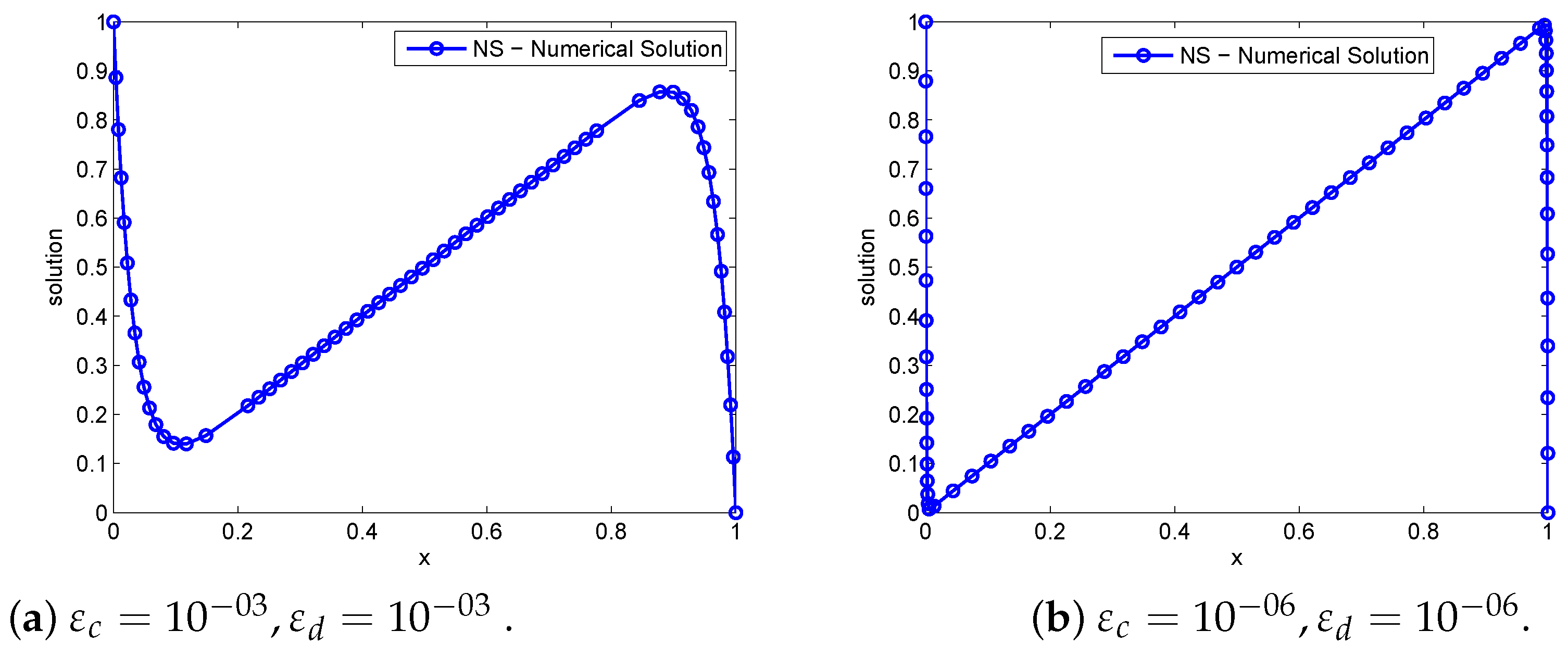
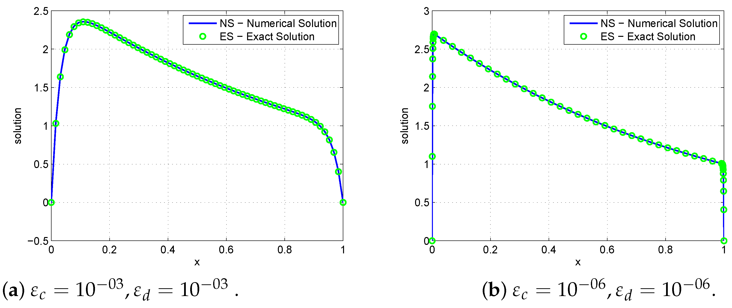
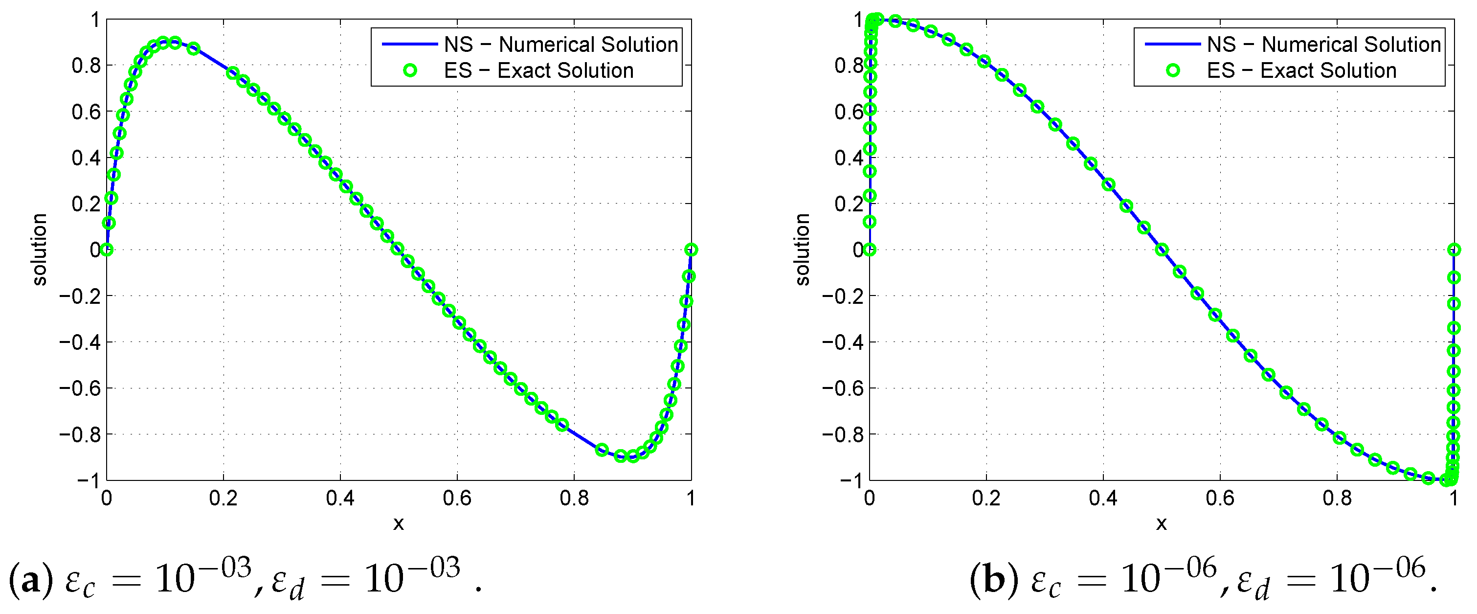
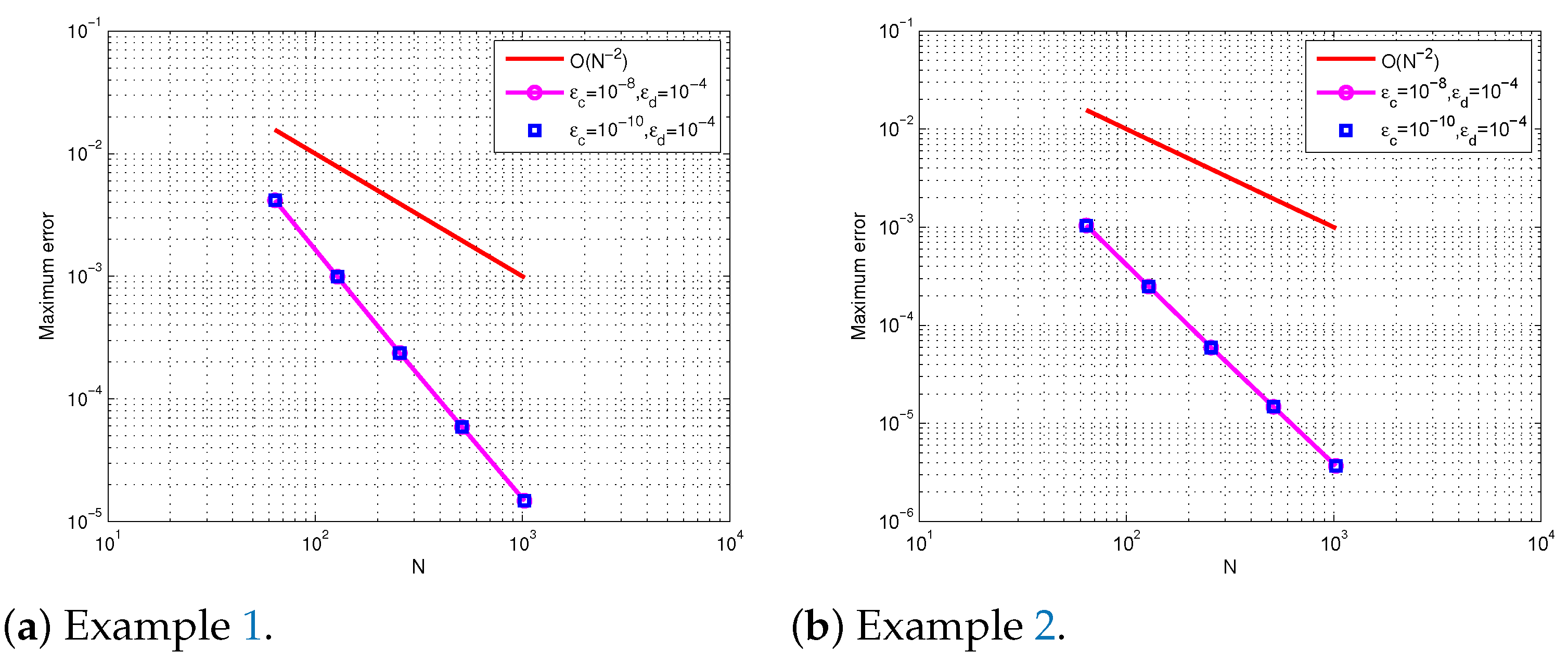
Numerical results in Table 1, Table 2, Table 3 and Table 4 confirm that the present method is uniformly convergent for Examples 1–4, respectively. Figure 1, Figure 2, Figure 3 and Figure 4 show numerical simulations for Examples 1–4. As ε c , ε d approaches very small values, we observe, in these Figures, that twin boundary layers at θ = 0 and θ = 1 were formed. The theoretical and numerical order of convergence are graphically shown by plotting the maximum absolute errors for Examples 1–2 and 3–4 using a log–log scale. This is demonstrated in Figure 5 and Figure 6, respectively, which demonstrate the parameter uniform convergence. The table of values below leads us to the conclusion that as the mesh points increase, the maximum absolute errors decrease.

6. Conclusions

A parameter uniformly convergent spline method is presented for singularly perturbed problems with two perturbation parameters. The governing differential equation is discretized using the spline method on a Bakhvalov-type mesh. The ( ε d , ε c ) -uniform convergence of the present method is well established. Based on the numerical solutions shown in the tables, this method is ( ε d , ε c ) uniformly convergent in the second-order. Graphs for the examples under consideration have been drawn using varying values of the parameters ε d and ε c in order to demonstrate the applicability of the present approach. Some comparisons have been given to consolidate the suitability of the present method.

Author Contributions

Conceptualization and formal analysis, H.J.A.S. and F.W.G.; methodology, software, visualization, and writing—original draft preparation, H.J.A.S., F.W.G. and A.A.A.G.; investigation, supervision, writing—review and editing, draft preparation, H.J.A.S., F.W.G. and A.A.A.G.; resources, project administration, funding acquisition, H.J.A.S. All authors have read and agreed to the published version of the manuscript.

Funding

This work was supported by the Deanship of Scientific Research, Vice Presidency for Graduate Studies and Scientific Research, King Faisal University, Saudi Arabia, Grant No. KFU252615.

Data Availability Statement

Data are contained within the article.

Acknowledgments

Authors are grateful to the referees for their valuable suggestions and comments.

Conflicts of Interest

The authors declare no conflicts of interest.

References

  1. O’Malley, R., Jr. Singular perturbations of boundary value problems for linear ordinary differential equations involving two parameters. J. Math. Anal. Appl. 1967, 19, 291–308. [Google Scholar] [CrossRef]
  2. O’Malley, R., Jr. Two-parameter singular perturbation problems for second-order equations. J. Math. Mech. 1967, 16, 1143–1164. [Google Scholar]
  3. Chen, J.; O’Malley, R., Jr. On the asymptotic solution of a two-parameter boundary value problem of chemical reactor theory. SIAM J. Appl. Math. 1974, 26, 717–729. [Google Scholar] [CrossRef]
  4. Vasil’Eva, A.B. Asymptotic methods in the theory of ordinary differential equations containing small parameters in front of the higher derivatives. USSR Comput. Math. Math. Phys. 1963, 3, 823–863. [Google Scholar] [CrossRef]
  5. DiPrima, R.C. Asymptotic methods for an infinitely long slider squeeze-film bearing. J. Lubr. Technol. 1968, 90, 173–183. [Google Scholar] [CrossRef]
  6. Bigge, J.; Bohl, E. Deformations of the bifurcation diagram due to discretization. Math. Comput. 1985, 45, 393–403. [Google Scholar] [CrossRef]
  7. Bhathawala, P.H.; Verma, A.P. A two-parameter singular perturbation solution of one dimension flow through unsaturated porous media. Appl. Math. 1975, 43, 380–384. [Google Scholar]
  8. Vulanovic, R.; Nhan, T.A. Robust hybrid schemes of higher order for singularly perturbed convection-diffusion problems. Appl. Math. Comput. 2020, 386, 125495. [Google Scholar] [CrossRef]
  9. Zhang, J.; Liu, X. Optimal order of uniform convergence for finite element method on Bakhvalov-type meshes. J. Sci. Comput. 2020, 85, 2. [Google Scholar] [CrossRef]
  10. Liu, X.; Zhang, J. Supercloseness of weak Galerkin method on Bakhvalov-type mesh for a singularly perturbed problem in 1D. Numer. Algorithms. 2023, 93, 367–395. [Google Scholar] [CrossRef]
  11. Zheng, Q.; Liu, Z. Uniform convergence analysis of a new adaptive upwind finite difference method for singularly perturbed convection-reaction-diffusion boundary value problems. J. Appl. Math. Comput. 2024, 70, 601–618. [Google Scholar] [CrossRef]
  12. Wondimu, F.; File, G.; Aga, T. Fourth order compact finite difference method for solving singularly perturbed 1D reaction diffusion equations with Dirichlet boundary conditions. Momona Ethiop. J. Sci. 2016, 8, 168–181. [Google Scholar] [CrossRef]
  13. Gelu, F.W.; Duressa, G.F.; Bullo, T.A. Tenth order compact finite difference method for solving singularly perturbed 1D reaction-diffusion equations. Int. J. Eng. Appl. Sci. 2016, 8, 15–24. [Google Scholar] [CrossRef]
  14. Gelu, F.W.; Duressa, G.F.; Bullo, T.A. Sixth-order compact finite difference method for singularly perturbed 1D reaction diffusion problems. J. Taibah Univ. Sci. 2017, 11, 302–308. [Google Scholar] [CrossRef]
  15. Ahmed, S.; Jahan, S.; Ansari, K.J.; Shah, K.; Abdeljawad, T. Wavelets collocation method for singularly perturbed differential-difference equations arising in control system. Results Appl. Math. 2024, 21, 100415. [Google Scholar] [CrossRef]
  16. Patidar, K.C. A robust fitted operator finite difference method for a two-parameter singular perturbation problem. J. Differ. Equ. Appl. 2008, 14, 1197–1214. [Google Scholar] [CrossRef]
  17. Shivhare, M.; Pramod Chakravarthy, P.; Kumar, D. Quadratic B-spline collocation method for two-parameter singularly perturbed problem on exponentially graded mesh. Int. J. Comput. Math. 2021, 98, 2461–2481. [Google Scholar] [CrossRef]
  18. Roos, H.-G.; Uzelac, Z. The SDFEM for a convection-diffusion problem with two small parameters. Comput. Methods Appl. Math. 2003, 3, 443–458. [Google Scholar] [CrossRef]
  19. Linss, T.; Roos, H.-G. Analysis of a finite-difference scheme for a singularly perturbed problem with two small parameters. J. Math. Anal. Appl. 2004, 289, 355–366. [Google Scholar] [CrossRef]
  20. Lodhi, R.K.; Jaiswal, B.R.; Nandan, D.; Ramesh, K. Numerical solution of two-parameter singularly perturbed convection-diffusion boundary value problems via fourth order compact finite difference method. Math. Model. Eng. Probl. 2021, 8, 819–825. [Google Scholar] [CrossRef]
  21. Kambampati, S.; Emineni, S.P.; Reddy, M.; Kolloju, P. Fourth order computational spline method for two-parameter singularly perturbed boundary value problem. Int. J. Appl. Mech. Eng. 2023, 28, 79–93. [Google Scholar] [CrossRef]
  22. Khandelwal, P.; Khan, A. Singularly perturbed convection-diffusion boundary value problems with two small parameters using nonpolynomial spline technique. Math. Sci. 2017, 11, 119–126. [Google Scholar] [CrossRef]
  23. O’Riordan, E.; Pickett, M.L. Numerical approximations to the scaled first derivatives of the solution to a two parameter singularly perturbed problem. J. Comput. Appl. Math. 2019, 347, 128–149. [Google Scholar] [CrossRef]
  24. Kadalbajoo, M.K.; Yadaw, A.S. B-spline collocation method for a two-parameter singularly perturbed convection-diffusion boundary value problems. Appl. Math. Comput. 2008, 201, 504–513. [Google Scholar] [CrossRef]
  25. Kadalbajoo, M.K.; Jha, A. Exponentially fitted cubic spline for two-parameter singularly perturbed boundary value problems. Int. J. Comput. Math. 2012, 89, 836–850. [Google Scholar] [CrossRef]
  26. Brdar, M.; Zarin, H. Convection-diffusion-reaction problems on a B-type mesh. PAMM Proc. Appl. Math. Mech. 2013, 13, 423–424. [Google Scholar] [CrossRef]
  27. Brdar, M.; Zarin, H. On graded meshes for a two-parameter singularly perturbed problem. Appl. Math. Comput. 2016, 282, 97–107. [Google Scholar] [CrossRef]
  28. Brdar, M.; Zarin, H. A singularly perturbed problem with two parameters on a Bakhvalov-type mesh. J. Comput. Appl. Math. 2016, 292, 307–319. [Google Scholar] [CrossRef]
  29. Andisso, F.S.; Duressa, G.F. Graded mesh B-spline collocation method for two parameters singularly perturbed boundary value problems. MethodsX 2023, 11, 102336. [Google Scholar] [CrossRef]
  30. Cheng, Y. On the local discontinuous Galerkin method for singularly perturbed problem with two parameters. J. Comput. Appl. Math. 2021, 392, 113485. [Google Scholar] [CrossRef]
  31. Agmas, A.F.; Gelu, F.W.; Fino, M.C. A robust, exponentially fitted higher-order numerical method for a two-parameter singularly perturbed boundary value problem. Frontiers Appl. Math. Stat. 2025, 10, 1501271. [Google Scholar] [CrossRef]
  32. Doolan, E.P.; Miller, J.J.; Schilders, W.H. Uniform Numerical Methods for Problems with Initial and Boundary Layers; Boole Press: Dublin, Ireland, 2000. [Google Scholar]
  33. Surla, K.; Uzelac, Z.; Teofanov, L. The discrete minimum principle for quadratic spline discretization of a singularly perturbed problem. Math. Comput. Simul. 2009, 79, 2490–2505. [Google Scholar] [CrossRef]
  34. Kumar, D. A uniformly convergent scheme for two-parameter problems having layer behaviour. Int. J. Comput. Math. 2022, 99, 553–574. [Google Scholar] [CrossRef]
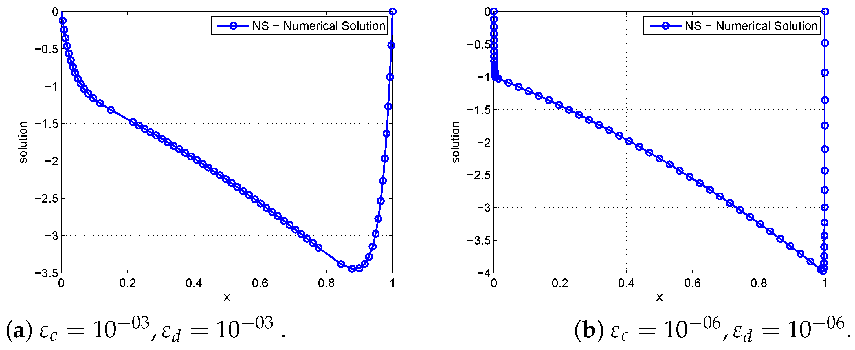
Figure 1. Solution behaviour using N = 64 for Example 1.
Axioms 14 00547 g001
Figure 2. Solution behaviour using N = 64 for Example 2.
Axioms 14 00547 g002
Figure 3. Solution behaviour using N = 64 for Example 3.
Axioms 14 00547 g003
Figure 4. Solution behaviour using N = 64 for Example 4.
Axioms 14 00547 g004
Figure 5. Plot of the maximum errors using the log–log scale for Examples 1 and 2.
Axioms 14 00547 g005
Figure 6. Plot of the maximum errors using the log–log scale for Examples 3 and 4.
Axioms 14 00547 g006
Table 1. Computations of e ε d , ε c N , e N , ρ ε d , ε c N and ρ N for Example 1 using ε d = 10 04 for varying values of ε c .
ε c N = 16 32641282565121024
Ours
10 04 6.8747 × 10 2 1.6838 × 10 2 4.0666 × 10 3 9.7083 × 10 4 2.3231 × 10 4 5.7900 × 10 5 1.4465 × 10 5
2.02962.04982.06652.06322.00442.0010
10 06 7.0732 × 10 2 1.7286 × 10 2 4.1640 × 10 3 9.9101 × 10 4 2.3688 × 10 4 5.9029 × 10 5 1.4747 × 10 5
2.03282.05362.07102.06472.00472.0010
10 08 7.0752 × 10 2 1.7290 × 10 2 4.1650 × 10 3 9.9121 × 10 4 2.3693 × 10 4 5.9040 × 10 5 1.4750 × 10 5
2.03282.05352.07112.06472.00472.0010
10 10 7.0752 × 10 2 1.7290 × 10 2 4.1650 × 10 3 9.9121 × 10 4 2.3693 × 10 4 5.9040 × 10 5 1.4750 × 10 5
2.03282.05352.07112.06472.00472.0010
e N 7.0752 × 10 2 1.7290 × 10 2 4.1650 × 10 3 9.9121 × 10 4 2.3693 × 10 4 5.9040 × 10 5 1.4750 × 10 5
ρ N 2.03282.05352.07112.06472.00472.0010
In [33]
e N -8.534 × 10 2 2.907 × 10 2 8.742 × 10 3 2.807 × 10 3 8.777 × 10 4 2.698 × 10 4
ρ N -1.5541.7331.6391.6771.702
Table 2. Computations of e ε d , ε c N , e N , ρ ε d , ε c N and ρ N for Example 2 using ε d = 10 04 for varying values of ε c .
ε c N = 16 32641282565121024
10 04 1.7916 × 10 2 4.3753 × 10 3 1.0529 × 10 3 2.5021 × 10 4 5.9810 × 10 5 1.4903 × 10 5 3.7233 × 10 6
2.03382.05502.07322.06472.00482.0009
10 06 1.7689 × 10 2 4.3228 × 10 3 1.0413 × 10 3 2.4782 × 10 4 5.9235 × 10 5 1.4761 × 10 5 3.6877 × 10 6
2.03282.05362.07102.06482.00472.0010
10 08 1.7687 × 10 2 4.3223 × 10 3 1.0412 × 10 3 2.4779 × 10 4 5.9229 × 10 5 1.4759 × 10 5 3.6873 × 10 6
2.03282.05362.07112.06472.00472.0010
10 10 1.7687 × 10 2 4.3223 × 10 3 1.0412 × 10 3 2.4779 × 10 4 5.9229 × 10 5 1.4759 × 10 5 3.6873 × 10 6
2.03282.05362.07112.06472.00472.0010
e N 1.7916 × 10 2 4.3753 × 10 3 1.0529 × 10 3 2.5021 × 10 4 5.9810 × 10 5 1.4903 × 10 5 3.7233 × 10 6
ρ N 2.03382.05502.07322.06472.00482.0009
Table 3. Computations of e ε d , ε c N , e N , ρ ε d , ε c N and ρ N for Example 3 using ε d = 10 04 for varying values of ε c .
ε c N = 16 32641282565121024
Ours
10 04 8.1690 × 10 2 1.8710 × 10 2 4.2318 × 10 3 9.5562 × 10 4 2.1847 × 10 4 5.4095 × 10 5 1.3500 × 10 5
2.12632.14452.14682.12902.01392.0025
10 06 8.0733 × 10 2 1.8499 × 10 2 4.1868 × 10 3 9.4644 × 10 4 2.1638 × 10 4 5.3576 × 10 5 1.3371 × 10 5
2.12572.14352.14532.12892.01392.0025
10 08 8.0724 × 10 2 1.8497 × 10 2 4.1863 × 10 3 9.4635 × 10 4 2.1636 × 10 4 5.3571 × 10 5 1.3370 × 10 5
2.12572.14352.14522.12892.01392.0025
10 10 8.0724 × 10 2 1.8497 × 10 2 4.1863 × 10 3 9.4635 × 10 4 2.1636 × 10 4 5.3571 × 10 5 1.3370 × 10 5
2.12572.14352.14522.12892.01392.0025
e N 8.1690 × 10 2 1.8710 × 10 2 4.2318 × 10 3 9.5562 × 10 4 2.1847 × 10 4 5.4095 × 10 5 1.3500 × 10 5
ρ N 2.12632.14452.14682.12902.01392.0025
In [34]
e N -4.4699 × 10 3 1.5184 × 10 3 7.8068 × 10 4 2.9511 × 10 4 8.6431 × 10 5 1.7362 × 10 5
Table 4. Computations of e ε d , ε c N , e N , ρ ε d , ε c N and ρ N for Example 4 using ε d = 10 06 for varying values of ε c .
ε c N = 16 32641282565121024
10 04 4.4492 × 10 2 9.4575 × 10 3 2.4671 × 10 3 5.6751 × 10 4 1.3067 × 10 4 3.1987 × 10 5 9.9258 × 10 6
2.07292.09982.12012.11872.03041.6882
10 06 3.9665 × 10 2 9.4465 × 10 3 2.2047 × 10 3 5.0753 × 10 4 1.1731 × 10 4 2.9113 × 10 5 9.3317 × 10 6
2.07002.09922.11902.11322.01061.6415
10 08 3.9620 × 10 2 9.4358 × 10 3 2.2022 × 10 3 5.0696 × 10 4 1.1719 × 10 4 2.9085 × 10 5 9.3259 × 10 6
2.07002.09922.11902.11302.01051.6410
10 10 3.9619 × 10 2 9.4357 × 10 3 2.2022 × 10 3 5.0695 × 10 4 1.1719 × 10 4 2.9085 × 10 5 9.3259 × 10 6
2.07002.09922.11902.11302.01051.6410
e N 4.4492 × 10 2 9.4575 × 10 3 2.4671 × 10 3 5.6751 × 10 4 1.3067 × 10 4 3.1987 × 10 5 9.9258 × 10 6
ρ N 2.07292.09982.12012.11872.03041.6882
Disclaimer/Publisher’s Note: The statements, opinions and data contained in all publications are solely those of the individual author(s) and contributor(s) and not of MDPI and/or the editor(s). MDPI and/or the editor(s) disclaim responsibility for any injury to people or property resulting from any ideas, methods, instructions or products referred to in the content.