The Generalized Multistate Complex Network Contagion Dynamics Model and Its Stability

Abstract

In this paper, we propose a new and fairly general network-based contagion dynamics model framework. In the model framework, each node in the network can be in one of multiple secure (or good) and infected (or bad) states. We characterize the dynamics of our model framework, by presenting the following: (i) a sufficient condition under which the dynamics are globally asymptotically stable; (ii) a sufficient condition under which the dynamics are locally asymptotically stable; and (iii) a sufficient condition for the persistence of bad states. Finally, we implemented three operations on the transition diagram. These three operations can help eliminate the bad states and help the model achieve the stability conditions.

1. Introduction

The processes such as the spread of computer viruses among computer nodes and the transmission of neural signals between neurons can all be regarded as interactions between nodes in a network. These interactions can be described using contagion dynamics on complex networks [1].

In fields such as epidemiology, social science, and cybersecurity, numerous complex network contagion dynamics models have been proposed to describe various complex contagion processes. In the field of cybersecurity, Wang et al. noticed the characteristics of complex networks in cyberspace and explicitly incorporated network topology into epidemic dynamics equations to study the spread of computer viruses in networks in their work [2]. Xu and Lu proposed a series of complex network epidemic dynamics models based on different cyber attack and defense strategies, including the preventive and reactive network defense dynamics models [3,4], and the proactive defense dynamics models [5,6], etc. In the field of opinion propagation, Zhang et al. proposed a complex network contagion dynamics model based on the SIS (susceptible-infected-susceptible) model [7] to study the impact of network structure on the diffusion of opinions, beliefs, and ideas in social networks [8]. She et al. proposed a coupled dynamics of epidemic spreading and opinion evolution in community networks to investigate the impact of opinion propagation on the evolution of epidemic states [9].

The aforementioned models can all be regarded as improvements and extensions of the classical epidemic dynamics model, the SIS (susceptible-infected-susceptible) model [7]—in these models, there are only two states: a good state and a bad state. The good state functions normally and is not infectious, while the bad state may cause harm to the system and has the ability to infect other nodes. However, as the understanding of various contagion processes deepens, researchers have realized that models with only two states are no longer sufficient to fully characterize the complex interaction mechanisms in the real world.

For example, some epidemics may have an incubation period, during which the state cannot be simply equated with the susceptible state; multiple pathogens may coexist in the same host, exhibiting different symptoms of infection [10]. Similarly, computer viruses can cause different types of damage when they attack different layers of a computer system. For example, a computer virus can cause damage to the operating system, the application layer, or the network layer of a computer system. If a virus attacks the operating system layer of a computer, it can cause the system to run unstably and frequently crash [11]; if a virus attacks the application software layer, it may tamper with software functions, steal user data, or exploit software vulnerabilities for contagion [12]; and if a virus attacks the network layer of a computer, it can spread via the network, steal sensitive information from network traffic, or launch distributed denial-of-service attacks (DDoS) [13]. In addition, multiple different computer viruses may also compete for computing resources on a single computer node [14].

Therefore, models with multiple good states and multiple bad states are more likely to capture the underlying patterns of general contagion processes. Before the impact of network structure on dynamics was recognized, several multi-state compartmental models of epidemic dynamics had already been proposed. In the classic textbook [15], Anderson systematically elaborated the SEIR (susceptible-exposed-infected-recovered) model framework with four states for studying epidemics with latent periods, such as tuberculosis and viral respiratory infections, as well as the SEAIR (susceptible-exposed-asymptomatic-infected-recovered) model with five states for studying diseases with asymptomatic carriers, such as HIV/AIDS. There are also some studies that have proposed multi-state complex network epidemic dynamics models. Liu et al. proposed a model with one good state and multiple bad states in their work [16]. Basnarkov studied the spread of COVID-19 using the SEAIR model on complex networks [17].

However, the aforementioned models all have a specific number of good states and bad states (for example, the SEIR model has two good states and two bad states), and the transition forms between each state are deterministic. This means that these models can only characterize the complex network contagion processes under specific scenarios. For a new contagion process, we need to establish a new mathematical model and re-propose the corresponding dynamical theory. If a unified complex network contagion dynamics modeling framework could be constructed, such that no matter how the number of states in the newly proposed model increases or how the transitions between states are defined, they can all be accommodated within this unified framework, and the dynamical theory of the new model can also be derived from the dynamical theory under this unified framework, then this would greatly promote the systematic and standardized development of research on complex network epidemic dynamics. The contributions of this chapter are as follows:

• Our Contributions.

• A new framework for complex network contagion dynamics models is proposed, which can accommodate any number of good states and bad states. Moreover, the specific mathematical form of node interactions in the network is not restricted, meaning that various forms of contagion processes can be discussed within this model. The dynamics of the model are characterized as follows: sufficient conditions for the extinction of bad states under any infection state are provided; the epidemic threshold of the model is derived using the method of lateral stability; and sufficient conditions for the persistence of bad states are also given. The model and its corresponding theory in this chapter are universal and can encompass four existing multi-state complex network epidemic dynamics frameworks and their corresponding theories.
• Three operations on the state transition diagram are proposed to help eliminate the bad states in the system and help the model achieve stability conditions. The effectiveness of these three operations is demonstrated using perturbation theory when the magnitude of the operations is small.
• The theoretical results were validated through numerical simulations on real network data.

It should be noted that the significance of this paper lies in summarizing the existing complex network contagion dynamics models and proposing a generalized modeling framework, rather than a mathematical model for a specific propagation process. Our work focuses more on theoretical analysis, rather than empirical application. For the verification of the theorems, we conducted numerical validation using real network data for the following reasons: (i) To the best of the authors’ knowledge, there are currently no datasets on contagion dynamics that consider complex networks. Existing datasets all lack network topology information, making it impossible to verify the gap between the model and real data. (ii) This paper focuses more on theoretical analysis and proposes a general theoretical framework that can accommodate existing models. This framework can include an arbitrary number of states. Therefore, even if there were real datasets, they could only validate specific cases of our model, which would not be very meaningful.

• Paper Outline.

Section 2 provides some mathematical preliminaries. Section 3 defines the basic concepts of the model and presents the master equations. Section 4 offers the theoretical results of our model. Section 5 validates these theoretical results through numerical experiments. Section 6 summarizes the paper and proposes future research directions. We have placed the main mathematical notations in

Table 1. Main notations used throughout the paper.

Notation	Description
#, $Re(·)$, $|·|$	# the size of a set; $Re(·)$ the real part of a complex number; $|·|$ the modulus of a complex number or the absolute value of a real number
$\mathrm{diag}\{·\}$	$\mathrm{diag}\{w_1,\dots ,w_d\}$ is a diagonal matrix with diagonal elements $w_1,\dots ,w_d$
${\mathbb{R}}_{\ge 0}$	the set of non-negative real numbers
${\lambda }_{H,\ell }$	the ℓ-th eigenvalue of $d\times d$ matrix H in the descending order of their real parts, $Re({\lambda }_{H,1})\ge Re({\lambda }_{H,2})\ge \dots \ge Re({\lambda }_{H,d})$
G, A	directed graph $G=(V,E)$ and its adjacency matrix
$\mathcal{G}$, $\mathcal{B}$, $\mathcal{S}$, n, m	$\mathcal{G}$ is the set of n good states; $\mathcal{B}$ is the set of m bad states; $\mathcal{S}=\mathcal{G}\cup \mathcal{B}$
$I_d$, $\mathbf{0}$	$I_d$ is the d-dimension identity matrix; $\mathbf{0}$ is the zero matrix
⊙	the Hadamard product (element-wise product between matrices)
$O(·)$	infinitesimals of the same order
$\sigma (·)$$\rho (·)$	the set of eigenvalues of a matrix, the spectral radius of a matrix
${\xi }_u(t)\in \mathcal{S}$	state of node u at time t
$p_{v,i,j}$, $P_{i,j}$	the neighbor-independent transition rate of node v where $i\in \mathcal{B}$ and $j\in \mathcal{S}$, and $P_{i,j}=\mathrm{diag}\{p_{1,i,j},\dots ,p_{k,i,j}\}$
${\delta }_{v,i}$, ${\delta }_i$	the probability that Type 1 bad-to-bad transition occurs on node v where $i\in \mathcal{B}$ and ${\delta }_i=\mathrm{diag}\{{\delta }_{1,i},{\delta }_{2,i},\dots ,{\delta }_{k,i}\}$
${\gamma }_{u,v}^{(i,l,j)}$, ${\mathsf{\Gamma }}_{i,l,j}$	the transition rate that node u in state $l\in \mathcal{B}$ attacks node v in state $i\in \mathcal{S}$ to cause v’s state changes from i to $j\in \mathcal{B}$, ${\mathsf{\Gamma }}_{i,l,j}={({\gamma }_{u,v}^{(i,l,j)})}_{k\times k}$
${\theta }_{v,i,j}(t)$	the transition rate that the state of node v is $i\in \mathcal{S}$ at time t and becomes $j\in \mathcal{B}$ at time $t+\Delta t$ as $\Delta t\to 0$.
$\mathcal{M}$	manifold {$w=(w_1,\dots ,w_{k(n+m)})\in {\mathbb{R}}_{\ge 0}^{k(n+m)}$ $\mid {\displaystyle \sum _{i=1}^{(n+m)}}{w}_{k(i-1)+v}=1$ for $v\in V=\{1,\dots ,k\}$}
$\mathcal{N}$	manifold $\{w=(w_1,\dots ,w_{k(n+m)})\in \mathcal{M}$ $\mid w_{\ell }=0$ for $\ell =kn+1,\dots ,k(n+m)$}
$x^{*}$	the fixed point on $\mathcal{N}$
$x_{v,i},x_{v,i}^{*}$, $x_i^{*}$	$x_{v,i}$ is the probability that node $v\in V$ is in state $i\in \mathcal{S}$ at time t, $x_{v,i}^{*}$ is the i-th entry of the fixed point of System (2), and $x_i^{*}=\mathrm{diag}\{x_{1,i}^{*},\dots ,x_{k,i}^{*}\}$
$D_{n,m}$	the Jacobian matrix of System (2)
${\mathbb{1}}_{·}$	Indicator function

for easy reference.

• Related Work.

Some of the existing literature has already made attempts in the direction of establishing a unified framework for complex network contagion dynamics. We use the term “good state” to refer to the state of not being infected by a virus or functioning normally, and the term “bad state” to refer to the state of being infected by a virus, unable to function properly, or having the ability to infect other nodes. For example, in the SIS model [7], the "S" state represents the good state, while the "I" state represents the bad state.

Xu et al. proposed a continuous-time general multivirus dynamics model for the spreading of multiple viruses in arbitrary networks [18]. The model features one good state and multiple bad states, where the good states can rob the bad state as well as other bad states. The model is homogeneous in terms of node parameters (i.e., the parameters of the model are the same for each node). The literature provides a sufficient condition for the extinction of all bad states.

Prakash et al. proposed a discrete-time dynamical model, $S^{*}{I}^{2}V$, based on undirected graphs and node homogeneous parameters, which includes two bad states and multiple other states. They derived the general epidemic threshold condition within this model and verified the generality of the epidemic threshold condition in models such as SEIR [19].

Paré et al. proposed a discrete-time dynamical model based on directed graphs, with heterogeneous node parameters (each node has different parameters), featuring one good state and multiple bad states. They also provided a global stability condition for a fixed point where all bad states disappear [16].

Sahneh et al. proposed a generalized epidemic mean-field model (GEMF) based on multilayer arbitrary networks with homogeneous node parameters and demonstrated the model’s generalization ability by showing that it can accommodate SIS, SIR, SAIS, and multi-pathogen infection models [20].

2. Preliminaries

2.1. Concepts and Properties About (Algebraic) Graph Theory and Real Matrices

Definition 1

(Directed graph). A directed graph can be defined as $G=(V,E)$, where V is the vertex or node set and $E\subseteq V\times V$ is the arc set. $(u,v)\in E$ is a arc from node u to node v, and we say node u is an incoming neighbor of node v and node v is an outgoing neighbor of node u.

Let function $Re(·)$ return the real part of a complex number and by $|·|$ the absolute value of a scalar variable. For a real matrix $H\in {\mathbb{R}}^{d\times d}$, denote by $\sigma (H)$ its set of eigenvalues and arrange its eigenvalues based on their real parts in the descending order, namely $Re({\lambda }_{H,1})\ge Re({\lambda }_{H,2})\ge \dots \ge Re({\lambda }_{H,d})$, where ${\lambda }_{H,\ell }$ for $\ell \in \{1,2,\dots ,d\}$ is the ℓ-th eigenvalue in this order. The spectral radius of H is $\rho (H)={\displaystyle \underset{\lambda \in \sigma (H)}{max}}\left|\lambda \right|$.

Definition 2

(Irreducible matrix). A matrix $H\in {\mathbb{R}}^{d\times d}$ is said to be irreducible if there is no permutation matrix $P\in {\mathbb{R}}^{d\times d}$ such that $P^{-1}HP$ is block upper triangular.

For two real matrices $H^{\prime }={(h_{u,v}^{\prime })}_{d\times d}\in {\mathbb{R}}^{d\times d}$ and $H^{″}={(h_{u,v}^{″})}_{d\times d}\in {\mathbb{R}}^{d\times d}$, we write $H^{\prime }\ge H^{″}$ if $h_{u,v}^{\prime }\ge h_{u,v}^{″}$ for all $u,v\in \{1,\dots ,d\}$. We say a vector is positive if all of its elements (or entries) are positive.

2.2. Concepts and Properties About Dynamical Systems

Consider a general d-dimensional dynamical system

$${\displaystyle \frac{dx(t)}{dt}}=f(x),$$

(1)

where $f(·)=(f_1,\dots ,f_d):{\mathbb{R}}^d\to {\mathbb{R}}^d$ and $f_i$ is continuously differentiable function on ${\mathbb{R}}^d$, and $x_e$ is a fixed point of System (1) such that $f(x_e)=\mathbf{0}$. We present several definitions regarding the stability of $x_e$. Let $\parallel ·\parallel$ denote the 2-norm on ${\mathbb{R}}^d$.

Definition 3

(Fixed-point Lyapunov stablility [21]). We say $x_e$ is Lyapunov-stable if, for any $ϵ>0$, there exists some $\delta =\delta (ϵ)>0$ such that for any other solution $x(t)$ to Equation (1) that satisfies $\parallel x_e-x\left(0\right)\parallel <\delta$, then $\parallel x_e-x(t)\parallel <ϵ$ for $t>0$.

Definition 4

(Locally asymptotic stability vs. Globally asymptotic fixed-point stability [21]). We say $x_e$ is locally asymptotically stable if it is Lyapunov-stable and there exists a constant $ϵ>0$; for any other solution $x(t)$ such that if $\parallel x_e-x\left(0\right)\parallel <ϵ$, then ${lim}_{t\to \infty }\parallel x_e-x(t)\parallel =0$. We say $x_e$ is globally asymptotically stable if it is Lyapunov-stable and for any other solution $x(t)$, ${lim}_{t\to \infty }\parallel x_e-x(t)\parallel =0$. If there are positive constants a and b, for any initial value $x(0)$ in a neighbor of $x_e$, $\parallel x(t)-x_e\parallel \le a\parallel x(0)-x_e\parallel e^{-bt}$ for $t\ge 0$, then $x_e$ is asymptotically stable with exponential speed.

For $f(x)$ in System (1), define

$$Df(x^{\prime })={\left.\left(\begin{array}{ccc}{\displaystyle \frac{\partial f_1}{\partial x_1}}& \dots & {\displaystyle \frac{\partial f_1}{\partial x_d}}\\ ⋮& & ⋮\\ {\displaystyle \frac{\partial f_d}{\partial x_1}}& \dots & {\displaystyle \frac{\partial f_d}{\partial x_d}}\end{array}\right)\right|}_{x=x^{\prime }}$$

as the Jacobian matrix of f at the point $x^{\prime }$.

Definition 5

(Spectrum of Lyapunov exponents [21]). Denote by $x(t,x_0)$ a trajectory of System (1) with initial value $x_0$ and by $\mathbf{h}\in {\mathbb{R}}^d$ a vector. Consider the linearization of System (1): $\dot{y(t)}=Df(x(t,x_0))y(t),$ and denote $X(t;x(t,x_0))$ as the fundamental solution matrix of the system. The Lyapunov exponent of trajectory $x(t,x_0)$ in the direction $\mathbf{h}$ is defined as $\chi \left(x\left(t,x_0\right),\mathbf{h}\right)\equiv {\overline{lim}}_{t\to \infty }{\displaystyle \frac{1}{t}}log{\displaystyle \frac{\parallel X\left(t;x\left(t,x_0\right)\right)\mathbf{h}\parallel }{\parallel \mathbf{h}\parallel }}.$ The set ${\{\chi \left(x\left(t,x_0\right),\mathbf{h}\right)\}}_{\begin{array}{c}\mathbf{h}\in {\mathbb{R}}^d,\\ \mathbf{h}\ne \mathbf{0}\end{array}}$ is called the Lyapunov exponents associated with $x\left(t,x_0\right)$.

We need to utilize some classical results regarding the asymptotic stability and comparison theorems of systems of ordinary differential equations with constant coefficients.

Lemma 1

([22]). System ${\displaystyle \frac{d}{dt}}x(t)=Cx(t)$, with $x(t)\in {\mathbb{R}}^d$ and $C\in {\mathbb{R}}^{d,d}$, is globally asymptotically stable with exponential speed if and only if the real part of every eigenvalue of C is negative.

Lemma 2

([18]). Consider a vector variable $x(t)={\left[x_1(t),\dots ,x_d(t)\right]}^{\top }\in$${\mathbb{R}}^n$ satisfying ${\displaystyle \frac{d}{dt}}{x}_i(t)\le {\sum }_{j=1}^d{c}_{ij}{x}_j(t),\forall i=1,\dots ,d,t\ge 0,$ where $c_{ij}\ge 0$ for all $i\ne j$. Furthermore, consider the following comparison system: ${\displaystyle \frac{d}{dt}}{y}_i(t)={\sum }_{j=1}^d{c}_{ij}{y}_j(t),\forall i=1,\dots ,d,t\ge 0.$ If $x_i(0)\le y_i(0)$ for all $i=1,\dots ,d$, then $x_i(t)\le y_i(t)$ holds for all $i=1,\dots ,d$ and $t\ge 0$.

Lemma 3 says that if the trajectory is a fixed point, the spectra of Lyapunov exponents are the real parts of the eigenvalues of the Jacobi matrix of System (1) at the fixed point.

Lemma 3

([21]). If the solution $x(t,x_0)$ is the fixed-point $x_e$, then the spectrum of the Lyapunov exponents of $x_e$ are the real parts of $Df(x_e)$’s eigenvalues.

3. Model

Traditional epidemic models do not take network topology into account and mainly depict the changes in the number of people in different states over time. Therefore, the variables in these models are the number of nodes in each state at a given time, or the proportion of nodes in different states relative to the total population. For example, in the traditional SIS (susceptible-infected-susceptible) model [23], the variables $S(t)$ and $I(t)$ denote the proportions of susceptible and infected individuals at time t, respectively. When considering a specific network topology, we pay more attention to the interactions between each node and its adjacent nodes, as well as the impact of the specific network structure on the dynamical behavior. This cannot be characterized merely by the proportion of nodes in each state. Instead, the state of each individual node needs to be taken into account. The dynamical variables then transform into the probability state of each node: the probability that each node is in a certain state at time t. For example, in the network-based SIS model [24], $i_v(t)$ represents the probability that node v is in infected state at time t. This concept is reasonable and is widely used, as the nodes can represent buildings, cities, or countries instead of individuals [25].

Network-based epidemic dynamics modeling is generally divided into two approaches: discrete-time and continuous-time. In the discrete-time model proposed by Chakrabarti et al., the model parameters represent the transition probabilities between states [26]. In contrast, in the continuous-time mean-field model proposed by Van Mieghem, the model parameters represent the aggregate rates of Poisson processes [27]. Although discrete-time models and continuous-time models are not equivalent, the forms of their transition equations are similar. Moreover, we can discretize the continuous-time model to draw conclusions similar to those of the discrete-time model, as in [16].

In this paper, we consider continuous-time dynamics taking place on a directed graph $G=(V,E)$, where $V=\{1,\dots ,k\}$ is the node set and E is the arc set. Denote by $A={(a_{u,v})}_{k\times k}$ the adjacent matrices of G, where $a_{u,v}=1$ if $(u,v)\in E$ and $a_{uv}=0$ otherwise. At any point in time, a node is in one of $n+m$ states, which are divided into two classes: (i) The class composed of n good states. The nodes in the good states are functional and do not propagate the virus. The class of good stats is denoted by $\mathcal{G}=\{1,\dots ,n\}$. (ii) the class of m bad states that cause damages. The class of bad state is denoted by $\mathcal{B}=\{-1,\dots ,-m\}$. Let $\mathcal{S}=\mathcal{G}\cup \mathcal{B}$.

The state of node $v\in V$ at time t can be represented by random variable ${\xi }_v(t)$. Denote by $x_{v,i}(t)$ the probability that $v\in V$ is in state $i\in \mathcal{S}$ at time t, namely $x_{v,i}(t)=\mathbb{P}({\xi }_v(t)=i).$ Like the other literature [20,28], what we aim to construct is the state transition equations of $x_{v,i}(t)$. There are two kinds of state transitions: neighbor-independent vs. neighbor-dependent.

3.1. Neighbor-Independent Transitions

These transitions are independent of the neighbors of node, including the following: (i) good-to-good transition, or from a good state $i\in \mathcal{G}$ to another good state $j\in \mathcal{G}$ with a rate $p_{v,i,j}$, where $j\ne i$; (ii) bad-to-good transition, or from a bad state $j\in \mathcal{B}$ to a good state $i\in \mathcal{G}$ with a rate $p_{v,j,i}$; (iii) bad-to-bad (Type 1) transition, or from a bad state $j\in \mathcal{B}$ to another bad state $j^{\prime }\in \mathcal{B}$ with a rate $p_{v,j,j^{\prime }}$ and the transition is indeed incurred by neighbor-independent transition with conditional probability ${\delta }_{v,j}$. That is, bad-to-bad (Type 1) transition occurs with rate ${\delta }_{v,j}{p}_{v,j,j^{\prime }}$.

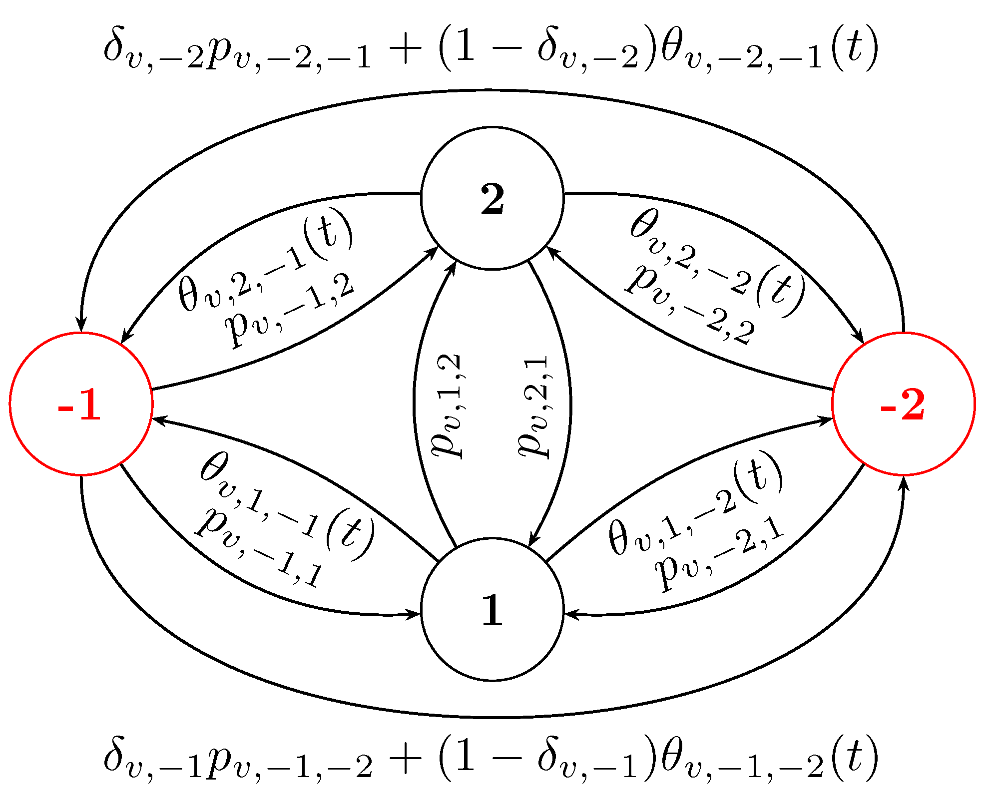
3.2. Neighbor-Dependent Transitions

The transitions that depend on the neighbors of a node include the following: (i) good-to-bad transition, or from a good state $i\in \mathcal{G}$ to a bad state $j\in \mathcal{B}$ with a time-dependent rate ${\theta }_{v,i,j}(t)$; (ii) bad-to-bad (Type 2) transition, namely from a bad state $j\in \mathcal{B}$ to another bad state $j^{\prime }\in \mathcal{B}$ with a rate ${\theta }_{v,j,j^{\prime }}(t)$, and the transition is indeed a neighbor-dependent transition with conditional probability $1-{\delta }_{v,j}$. That is, bad-to-bad (Type 2) transition occurs with rate $(1-{\delta }_{v,j}){\theta }_{v,j,j^{\prime }}(t)$.

Suppose that a node v in state $i\in \mathcal{G}$ (or in $j\in \mathcal{B}$) is infected by node u in state $l\in \mathcal{B}$ to state $j^{\prime }$ with rate ${\gamma }_{u,v}^{(i,l,j)}$ (or ${\gamma }_{u,v}^{(j,l,j^{\prime })}$). ${\theta }_{v,i,j}(t)$ (or ${\theta }_{v,j,j^{\prime }}(t)$) is the function of ${\gamma }_{u,v}^{(i,l,j)}$ (or ${\gamma }_{u,v}^{(j,l,j^{\prime })}$) and it reflects the aggregate effect of node v’s incoming neighbors in bad state $l\in \mathcal{B}$ on causing the state change to v, where each bad state l possibly serves as a “contributor” to the state transition of v. Denote by ${\mathsf{\Gamma }}_{i,l,j}={({\gamma }_{u,v}^{(i,l,j)})}_{k\times k}$. The specific form of ${\theta }_{v,i,j}(t)$ will be elaborated on later. Now we introduce the master state transition equations.

3.3. Master Equation

For $v\in V$, there are two class equations, one corresponding to good states and the other corresponding to bad states, leading to a system of $k(m+n)$ equations: for $v\in V$, $i\in \mathcal{G}$, and $j\in \mathcal{B}$:

$$\begin{array}{cc}\hfill {\displaystyle \frac{d}{dt}}{x}_{v,i}(t)=& {\displaystyle \sum _{j\in \mathcal{S},j\ne i}}{p}_{v,j,i}·x_{v,j}(t)-{\displaystyle \sum _{i^{\prime }\in \mathcal{G},i^{\prime }\ne i}}{p}_{v,i,i^{\prime }}·x_{v,i}(t)-{\displaystyle \sum _{j\in \mathcal{B}}}{\theta }_{v,i,j}(t)·x_{v,i}(t);\hfill \\ \hfill {\displaystyle \frac{d}{dt}}{x}_{v,j}(t)=& {\displaystyle \sum _{i\in \mathcal{G}}}{\theta }_{v,i,j}(t)·x_{v,i}(t)+{\displaystyle \sum _{j^{\prime }\in \mathcal{B}}}(1-{\delta }_{v,j^{\prime }}){\theta }_{v,j^{\prime },j}(t)·x_{v,j^{\prime }}(t)+{\displaystyle \sum _{j^{\prime }\in \mathcal{B}}}{\delta }_{v,j^{\prime }}{p}_{v,j^{\prime },j}·x_{v,j^{\prime }}(t)\hfill \\ \hfill -& {\displaystyle \sum _{i\in \mathcal{G}}}{p}_{v,j,i}·x_{v,j}(t)-{\displaystyle \sum _{j^{\prime }\in \mathcal{B},j^{\prime }\ne j}}{\delta }_{v,j}{p}_{v,j,j^{\prime }}·x_{v,j}(t)-{\displaystyle \sum _{j^{\prime }\in \mathcal{B},j^{\prime }\ne j}}(1-{\delta }_{v,j}){\theta }_{v,j,j^{\prime }}(t)x_{v,j}(t).\hfill \end{array}$$

(2)

The equations above may seem intricate. To provide a clearer understanding of the master equation, Figure 1 depicts a system featuring two good and two bad states, offering a visual aid to grasp the concept more easily. Suppose the good states are $\{1,2\}$ and the bad states are $\{-1,-2\}$. The diagram illustrates the transition rates of the probability of each state of any node to other states at time t. To facilitate distinction, we represent the bad states $-1$ and $-2$ with red nodes. For instance, the probability $x_{v,1}(t)$ of node v being in the good state 1 at time t transitions to state 2 at a rate of $p_{v,1,2}$. The transition rates to the bad states −1 and −2 are ${\theta }_{v,1,-1}(t)$ and ${\theta }_{v,1,-2}(t)$, respectively. Here, $p_{v,1,2}$ is the neighbor-independent transition of v, while ${\theta }_{v,1,-1}(t)$ and ${\theta }_{v,1,-2}(t)$ are the neighbor-dependent transitions. We refer to such a diagram as a state transition diagram.

3.4. Instantiating ${\theta }_{v,i,j}(t)$ to Accommodate Existing Models

In the literature, the forms of neighbor-dependent transition rate ${\theta }_{v,i,j}(t)$ for $i\in \mathcal{S}$, $j\in \mathcal{B}$ generally fall into two categories, we refer to them as:

• ∑-model [20,28], where ${\theta }_{v,i,j}(t)={\displaystyle \sum _{l\in \mathcal{B}}}{\displaystyle \sum _{u\in V}}{a}_{u,v}{\gamma }_{u,v}^{(i,l,j)}·x_{u,l}(t);$
• and ∏-model [4], where ${\theta }_{v,i,j}(t)={\displaystyle \sum _{l\in \mathcal{B}}}(1-{\displaystyle \prod _{u\in V}}(1-a_{u,v}{\gamma }_{u,v}^{(i,l,j)}·x_{u,l}(t))).$

When analyzing the properties of these models, such as the epidemic threshold, it is primarily the linear part of ${\theta }_{v,i,j}(t)$ that plays a role. It is easy to see that the linear parts of the ∑-model and the ∏-model are the same. This implies that when analyzing properties that are related only to the linear term of ${\theta }_{v,i,j}(t)$, the conclusions hold for both models. Therefore, we hope to find a way to define ${\theta }_{v,i,j}(t)$ that can accommodate both ∑-model and ∏-model, so that the conclusions derived within our model are universal.

Define

$${\theta }_{v,i,j}(t)={\displaystyle \sum _{l\in \mathcal{B}}}{\displaystyle \sum _{u\in V}}{a}_{u,v}{\gamma }_{u,v}^{(i,l,j)}·x_{u,l}(t)+R_{i,j}^v({\{x_{u,l}(t)\}}_{u\in V,l\in \mathcal{B}}),$$

(3)

where $R_{i,j}^v({\{x_{u,l}(t)\}}_{u\in V,l\in \mathcal{B}})$ is a function of $x_{u,l}(t)$ for $u\in V$ and $l\in \mathcal{B}$. When there is no ambiguity, we use $R_{i,j}^v$ to represent $R_{i,j}^v({\{x_{u,l}(t)\}}_{u\in V,l\in \mathcal{B}})$. To facilitate analysis, we require that ${\displaystyle \frac{\partial {\theta }_{v,i,j}(t)}{\partial x_{u,l}}}\ge 0$ and $R_{i,j}^v$ satisfies the following mathematical properties:

• $R_{i,j}^v$ is a continuously differentiable function with respect to $x_{u,l}(t)$.
• $R_{i,j}^v\le 0$ always hold and

  $$R_{i,j}^v=O\left({\displaystyle \sum _{l_1,l_2\in \mathcal{B}}}{\displaystyle \sum _{u_1,u_2\in V}}{a}_{u_1,v}{a}_{u_2,v}{x}_{u_1,l_1}{x}_{u_2,l_2}\right),$$

  (4)

  when $x_{u_1,l_1},x_{u_2,l_2}\to 0$, where $O(·)$ denotes the symbol for infinitesimals of the same order.

It is easy to show that the above ∑-model and ∏-model are special cases of our model: in ∑-model, $R_{i,j}^v=0$, and in ∏-model,

$$R_{i,j}^v=-{\displaystyle \sum _{l\in \mathcal{B}}}{\displaystyle \sum _{u_1,u_2\in V}}{\gamma }_{u_1,v}^{(i,l,j)}{\gamma }_{u_2,v}^{(i,l,j)}{a}_{u_1,v}{a}_{u_2,v}{x}_{u_1,l}{x}_{u_2,l}+O(x_{u,l}^3)$$

as all $x_{u,l}\to 0$. Therefore, the theoretical analysis of our model is also applicable to the analysis of the above two models.

4. Analysis

4.1. Sufficient Conditions for Global Stability

Note that ${\displaystyle \sum _{i\in \mathcal{S}}}{x}_{v,i}(0)=1$ and when $x_{v,i}(t)=0$, ${\displaystyle \frac{d{x}_{v,i}(t)}{dt}}\ge 0$, which means $x_{v,i}(t)\ge 0$. Define manifold $\mathcal{M}:$ {$w=(w_1,\dots ,w_{k(n+m)})\in {\mathbb{R}}_{\ge 0}^{k(n+m)}$$\mid {\displaystyle \sum _{i=1}^{(n+m)}}{w}_{k(i-1)+v}=1$ for $v=1,\dots ,k$}, which is smooth.

Lemma 4.

System (2) acts on the finite-dimension smooth manifold $\mathcal{M}$ defined above and leads to flow $\varphi (t,x):{\mathbb{R}}_{\ge 0}\times \mathcal{M}\to \mathcal{M}$ where $\varphi (0,w)=w$ and $w\in \mathcal{M}$.

The proof of Lemma 4 is referred to Appendix C. Lemma 4 shows that the solutions of System (2) always lie on the manifold $\mathcal{M}$.

Define a submanifold of $\mathcal{M}$ as $\mathcal{N}:\{w=(w_1,\dots ,w_{k(n+m)})\in \mathcal{M}$$\mid w_{\ell }=0$ for $\ell =kn+1,\dots ,k(n+m)$}. On $\mathcal{N}$, the probability of a node v in bad states, ${\displaystyle \sum _{j\in \mathcal{B}}}{x}_{v,j}(t)=0$, denotes the “ideal” scenario where all the bad states have vanished. For $v\in V$, define

$$G{G}_v=\left(\begin{array}{cccc}-{\displaystyle \sum _{j\in \mathcal{G},j\ne n}}{p}_{v,n,j}& p_{v,n-1,n}& \dots & p_{v,1,n}\\ p_{v,n,n-1}& -{\displaystyle \sum _{j\in \mathcal{G},j\ne n-1}}{p}_{v,n-1,j}& \dots & p_{v,1,n-1}\\ ⋮& ⋮& \ddots & ⋮\\ p_{v,n,1}& p_{v,n-1,1}& \dots & -{\displaystyle \sum _{j\in \mathcal{G},j\ne 1}}{p}_{v,1,j}\end{array}\right).$$

It is easy to see that 0 is an eigenvalue of $G{G}_v$, with the left eigenvector ${\mathbf{1}}_n^T$, which denotes the n-dimensional row vector with all components equal to 1, where $n=\#\mathcal{G}$. We make the following assumption based on $G{G}_v$:

Assumption 1.

For each $v\in V$, the eigenspace corresponding to the eigenvalue 0 of $G{G}_v$ is one-dimensional.

Assumption 1 is realistic and reasonable. For example, most contagion dynamics models in cybersecurity, such as the preventive and reactive cyber defense model [24,29], the multi-virus competing model [18], and the multivirus model [16], etc, have only one good state, in which $G{G}_v=[0]$, satisfying Assumption 1. The SEIR [15] model is a typical example of a model with multiple desirable states. It has desirable states denoted by “S” and “E”, with

$$G{G}_v=\left(\begin{array}{cc}-p_{2,1}& 0\\ p_{2,1}& 0\end{array}\right),$$

where $p_{2,1}$ is the transition rate at which nodes move from state “S” to state “E”. The eigenvalues of $G{G}_v$ is $-p_{2,1}$ and 0. Therefore, the SEIR model also satisfies Assumption 1.

Lemma 5 below shows that $\mathcal{N}$ is an invariant submanifold (of $\mathcal{M}$) and can have a unique asymptotically stable fixed point. Proof of Lemma 5 is deferred to in Appendix B.

Lemma 5.

Submanifold $\mathcal{N}$ is invariant under the flow of System (2), $\varphi (t,x):{\mathbb{R}}_{\ge 0}\times \mathcal{M}\to \mathcal{M}$. Moreover, if Assumption 1 is satisfied, $\mathcal{N}$ has a unique fixed-point $x^{*}$ under the map ${\varphi |}_{\mathcal{N}}$, where ${\varphi |}_{\mathcal{N}}$ means the flow ϕ only acts on the invariant submanifold $\mathcal{N}$.

Any infection situation in cyberspace can be represented by a point on the manifold $\mathcal{M}$. We call the point “manageable” if the point can be driven into $\mathcal{N}$ under the action of System (2), that is, into the “safe” situation free of viruses. To simplify notations, we denote $x_i^{*}=\mathrm{diag}\{x_{1,i}^{*},x_{2,i}^{*},\dots ,x_{k,i}^{*}\}$, where $x_{v,i}^{*}$ for $v\in V$ are the entries of the fixed-point $x^{*}$, $P_{i,j}=\mathrm{diag}\{p_{1,i,j},p_{1,i,j},\dots ,p_{k,i,j}\}$, and ${\delta }_i=\mathrm{diag}\{{\delta }_{1,i},{\delta }_{2,i},\dots ,{\delta }_{k,i}\}$. Define matrix $B_0$ as:

$$\begin{array}{cc}\hfill B_0& =\left(\begin{array}{cc}{\displaystyle \sum _{i\in \mathcal{G}}}{(A\odot {\mathsf{\Gamma }}_{i,-1,-1})}^T+{\displaystyle \sum _{j\in \mathcal{B},j\ne -1}}(I_k-{\delta }_j){(A\odot {\mathsf{\Gamma }}_{j,-1,-1})}^T-{\displaystyle \sum _{i\in \mathcal{G}}}{P}_{-1,i}-{\displaystyle \sum _{\begin{array}{c}j\in \mathcal{B}\\ j\ne -1\end{array}}}{\delta }_{-1}\odot P_{-1,j},& \dots \\ {\displaystyle \sum _{i\in \mathcal{G}}}{(A\odot {\mathsf{\Gamma }}_{i,-1,-2})}^T+{\displaystyle \sum _{\begin{array}{c}j\in \mathcal{B}\\ j\ne -1\end{array}}}(I_k-{\delta }_j){(A\odot {\mathsf{\Gamma }}_{j,-1,-2})}^T+{\delta }_{-1}\odot P_{-1,-2},& \dots \\ ⋮& \dots \\ {\displaystyle \sum _{i\in \mathcal{G}}}{(A\odot {\mathsf{\Gamma }}_{i,-1,-m})}^T+{\displaystyle \sum _{\begin{array}{c}j\in \mathcal{B}\\ j\ne -1\end{array}}}(I_k-{\delta }_j){(A\odot {\mathsf{\Gamma }}_{j,-1,-m})}^T+{\delta }_{-1}\odot P_{-1,-m},& \dots \end{array}\right.\hfill \\ \hfill & \left.\begin{array}{cc}\dots & {\displaystyle \sum _{i\in \mathcal{G}}}{(A\odot {\mathsf{\Gamma }}_{i,-m,-1})}^T+{\displaystyle \sum _{\begin{array}{c}j\in \mathcal{B}\\ j\ne -1\end{array}}}(I_k-{\delta }_j){(A\odot {\mathsf{\Gamma }}_{j,-m,-1})}^T+{\delta }_{-m}\odot P_{-m,-1}\\ \dots & {\displaystyle \sum _{i\in \mathcal{G}}}{(A\odot {\mathsf{\Gamma }}_{i,-m,-2})}^T+{\displaystyle \sum _{\begin{array}{c}j\in \mathcal{B}\\ j\ne -2\end{array}}}(I_k-{\delta }_j){(A\odot {\mathsf{\Gamma }}_{j,-m,-2})}^T+{\delta }_{-m}\odot P_{-m,-2}\\ ⋮\\ \dots & {\displaystyle \sum _{i\in \mathcal{G}}}{(A\odot {\mathsf{\Gamma }}_{i,-m,-m})}^T+{\displaystyle \sum _{\begin{array}{c}j\in \mathcal{B}\\ j\ne -m\end{array}}}(I_k-{\delta }_j){(A\odot {\mathsf{\Gamma }}_{j,-m,-m})}^T-{\displaystyle \sum _{i\in \mathcal{G}}}{P}_{-m,i}-{\displaystyle \sum _{\begin{array}{c}j\in \mathcal{B}\\ j\ne -m\end{array}}}{\delta }_{-m}\odot P_{-m,j}\end{array}\right).\hfill \end{array}$$

(5)

Theorem 1 below gives a sufficient condition under which System (2) goes into $\mathcal{N}$ and then converges to $\mathcal{N}$’s unique fixed-point $x^{*}$, meaning that all bad states vanish (i.e., making the dynamics “manageable” [30]). Its proof is deferred to in Appendix D.

Theorem 1

(Globally asymptotic stability). ${\lambda }_{B_0,1}$ is always real. Moreover, if Assumption 1 is satisfied and ${\lambda }_{B_0,1}<0$, then $\mathcal{N}$’s fixed-point $x^{*}$ is globally asymptotically stable with an exponential convergence speed.

As all $x_{v,i}\ge 0$, if for all $v\in V$, ${\displaystyle \sum _{j\in \mathcal{B}}}{x}_{v,j}(t)\to 0$ is equivalent to $x_{v,j}(t)\to 0$ for all $j\in \mathcal{B}$. Corollary 1 provides the sufficient condition under which ${\displaystyle \sum _{j\in \mathcal{B}}}{x}_{v,j}(t)\to 0$, and then each $x_{v,j}(t)\to 0$. It only requires the computation of the largest eigenvalue of a $k\times k$ matrix $m{\mathsf{\Theta }}_1-n{\mathcal{P}}_1$, thereby reducing the computational complexity. Its proof is in Appendix D.2.

Denote ${\mathsf{\Theta }}_1={[{\displaystyle \underset{\begin{array}{c}i\in \mathcal{G}\\ l,j\in \mathcal{B}\end{array}}{max}}\{{\gamma }_{u,v}^{(i,l,j)}\}{a}_{u,v}]}_{u\in V,v\in V}$, ${\mathcal{P}}_1=\mathrm{diag}\{{\displaystyle \underset{\begin{array}{c}j\in \mathcal{B}\\ i\in \mathcal{G}\end{array}}{min}}\{p_{1,j,i}\},\dots ,{\displaystyle \underset{\begin{array}{c}j\in \mathcal{B}\\ i\in \mathcal{G}\end{array}}{min}}\{p_{k,j,i}\}\}$.

Corollary 1.

If Assumption 1 is satisfied and $Re({\lambda }_{m{\mathsf{\Theta }}_1-n{\mathcal{P}}_1,1})<0$, $x^{*}$ is globally asymptotic stable.

If the parameters are node- and arc- independent, namely $p_{v,i,j}=p_{i,j}$, ${\gamma }_{u,v}^{(i,l,j)}={\gamma }^{(i,l,j)}$, ${\delta }_{v,i}={\delta }_{1,i}$ for $i,j,l\in \mathcal{S}$, $u,v\in V$, Corollary 2 decouples ${\lambda }_{A,1}$ from the condition ${\lambda }_{B_0,1}$. This simplifies the computational complexity: the calculation of the eigenvalues of the $mk\times mk$ matrix B is transformed into the calculation of the eigenvalues of a $k\times k$ matrix and an $m\times m$ matrix. The proof of Corollary 2 is deferred to in Appendix D.3.

Let $\mathsf{\Theta }={[{\mathsf{\Theta }}_{l,j}]}_{l\in \mathcal{B},j\in \mathcal{B}}$ where ${\mathsf{\Theta }}_{l,j}={\displaystyle \sum _{i\in \mathcal{G}}}{\gamma }^{(i,l,j)}+{\displaystyle \sum _{j^{\prime }\in \mathcal{B}}}(1-{\delta }_{1,j^{\prime }}){\gamma }^{(j^{\prime },l,j)}$, $\mathcal{P}={[{\delta }_{1,j}{p}_{j,j^{\prime }}]}_{j\in \mathcal{B},j^{\prime }\in \mathcal{B}}$, and ${\mathcal{P}}^{\prime }=\mathrm{diag}\{({\displaystyle \sum _{i\in \mathcal{G}}}{p}_{i,j}+{\displaystyle \sum _{j^{\prime }\in \mathcal{B},j^{\prime }\ne j}}{\delta }_{1,j^{\prime }}{p}_{j^{\prime },j}{)}_{j\in \mathcal{B}}\}$.

Corollary 2

(of Theorem 1). If Assumption 1 is satisfied and $max\{Re(\xi ):\xi \in \lambda ({\lambda }_{A,1}\mathsf{\Theta }+$$\mathcal{P}-{\mathcal{P}}^{\prime })\}$$<0,$ the unique fixed-point $x^{*}$ on $\mathcal{N}$ is globally asymptotically stable at an exponential convergence speed (i.e., all bad states vanish exponentially regardless of the initial value).

4.2. Sufficient Conditions for the Local Asymptotic Stability of $x^{*}$

Numerical experiments in Section 5.2 can illustrate that this condition is far from being a necessary condition. This condition is applicable for rapidly eliminating the virus during a large-scale outbreak. In what follows, we show that under a mild condition, $\mathcal{N}$’s fixed point $x^{*}$ is locally asymptotically stable on $\mathcal{M}$. Denote by $D_{n,m}$ the Jacobian matrix of System (2) at $x^{*}$. Then, we can find $D_{n,m}=\left(\begin{array}{c}\begin{array}{cc}GG& GB\\ \mathbf{0}& B\end{array}\end{array}\right),$ where (i) $GG$ is the $kn\times kn$ matrix obtained by differentiating the $kn$ equations in System (2) corresponding to the n good states $i\in \mathcal{G}$ at $x^{*}$; (ii) $GB$ is the $kn\times km$ matrix obtained by differentiating the $kn$ equations in System (2) corresponding to the m bad states $i\in \mathcal{B}$ at $x^{*}$; (iii) $\mathbf{0}$ is the $km\times kn$ zero matrix because the derivative of the equations in System (2) corresponding to the m bad states at $x^{*}$ is always 0 (owing to the fact that there are no neighbor-independent transitions from the n good states to the m bad states); and (iv) B is the $km\times km$ matrix obtained by differentiating the $km$ equations in System (2) corresponding to the m bad states $i\in \mathcal{B}$ at $x^{*}$.

In $D_{n,m}$, the useful elements for analysis are $GG$ and B, $GG=$

$$\left(\begin{array}{c}\begin{array}{cccc}-{\displaystyle \sum _{i\in \mathcal{G},i\ne n}}{P}_{n,i}& P_{n-1,n}& \dots & P_{1,n}\\ P_{n,n-1}& -{\displaystyle \sum _{i\in \mathcal{G},n-1}}{P}_{n-1,i}& \dots & P_{1,n-1}\\ ⋮& ⋮& ⋮& ⋮\\ P_{n,1}& \dots & P_{2,1}& -{\displaystyle \sum _{i\in \mathcal{G},i\ne 1}}{P}_{1,i}\end{array}\end{array}\right),$$

(6)

and $B=$

$$\left(\begin{array}{ccc}{\displaystyle \sum _{i\in \mathcal{G}}}{x}_i^{*}{(A\odot {\mathsf{\Gamma }}_{i,-1,-1})}^T-{\displaystyle \sum _{i\in \mathcal{G}}}{P}_{-1,i}-{\displaystyle \sum _{\begin{array}{c}j\in \mathcal{B}\\ j\ne -1\end{array}}}{\delta }_{-1}\odot P_{-1,j}& \dots & {\displaystyle \sum _{i\in \mathcal{G}}}{x}_i^{*}{(A\odot {\mathsf{\Gamma }}_{i,-m,-1})}^T+{\delta }_{-m}\odot P_{-m,-1}\\ {\displaystyle \sum _{i\in \mathcal{G}}}{x}_i^{*}{(A\odot {\mathsf{\Gamma }}_{i,-1,-2})}^T+{\delta }_{-1}\odot P_{-1,-2},& \dots & {\displaystyle \sum _{i\in \mathcal{G}}}{x}_i^{*}{(A\odot {\mathsf{\Gamma }}_{i,-m,-2})}^T+{\delta }_{-m}\odot P_{-m,-2}\\ ⋮& \dots & ⋮\\ {\displaystyle \sum _{i\in \mathcal{G}}}{x}_i^{*}{(A\odot {\mathsf{\Gamma }}_{i,-1,-m})}^T+{\delta }_{-1}\odot P_{-1,-m}& \dots & {\displaystyle \sum _{i\in \mathcal{G}}}{x}_i^{*}{(A\odot {\mathsf{\Gamma }}_{i,-m,-m})}^T-{\displaystyle \sum _{i\in \mathcal{G}}}{P}_{-m,i}-{\displaystyle \sum _{\begin{array}{c}j\in \mathcal{B}\\ j\ne -m\end{array}}}{\delta }_{-m}\odot P_{-m,j}\end{array}\right),$$

(7)

where ⊙ is the element-wise matrix product.

When analyzing the local stability at $x^{*}$, we only need to pay attention to the bad states (rather than all states, which are required in [16,31,32]). Theorem 2 below says that if $Re({\lambda }_{B,1})<0$, then the $\mathcal{N}$’s fixed-point $x^{*}$ on is locally asymptotically stable on $\mathcal{M}$. (Note that $\mathcal{N}$ has a unique fixed point does not necessarily mean the fixed point of $\mathcal{M}$ is also unique.)

Theorem 2

(Sufficient condition for locally asymptotic stability). ${\lambda }_{B,1}$ is always real. If Assumption 1 is satisfied and ${\lambda }_{B,1}<0$, then the fixed-point $x^{*}$ on $\mathcal{N}$ is also locally asymptotically stable on $\mathcal{M}$.

The proof can be obtained by applying Lemma 5, Lemma 3 and Theorem 2.12 in [33].

Remark 1.

Lemma 5 indicates that when there are no bad states in the system, the state of each node will remain at $x^{*}$. Theorem 2 shows that when ${\lambda }_{B,1}<0$, if the system experiences a small number of bad states (a few viruses are introduced into cyberspace by attackers), the system has a certain degree of resistance and can spontaneously clear these bad states without triggering a large-scale outbreak of virus spread.

Lemma 6 below formally shows that the condition for globally asymptotic stability, ${\lambda }_{B_0,1}<0$, is more restrictive than that for locally asymptotic stability, ${\lambda }_{B,1}<0$. Corollary 3 of Theorem 2 considers the case of homogeneous parameters, which allows us to decouple ${\lambda }_{A,1}$ from B and reduces the computational complexity. The proof of Lemma 6 and the proof of Corollary 3 are deferred to in Appendix E.

Lemma 6

(${\lambda }_{B,1}$ vs. ${\lambda }_{B_0,1}$). It holds that ${\lambda }_{B_0,1}\ge {\lambda }_{B,1}$.

Consider $\tilde{\mathsf{\Theta }}={[{\sum }_{i\in \mathcal{G}}{x}_{1,i}^{*}{\gamma }^{(i,l,j)}]}_{l\in \mathcal{B},j\in \mathcal{B}}$, $\mathcal{P}={[{\delta }_{1,j}{p}_{j,j^{\prime }}]}_{j\in \mathcal{B},j^{\prime }\in \mathcal{B}}$, and ${\mathcal{P}}^{\prime }=\mathrm{diag}\{({\displaystyle \sum _{i\in \mathcal{G}}}{p}_{j,i}+{\displaystyle \sum _{\begin{array}{c}{j}^{\prime }\in \mathcal{B}\\ j^{\prime }\ne j\end{array}}}{\delta }_{1,j}{p}_{j,j^{\prime }}{)}_{j\in \mathcal{B}}\}$.

Corollary 3

(of Theorem 2). If Assumption 1 is satisfied and

$$max\left\{Re(\xi ):\xi \in \lambda \left({\lambda }_{A,1}\tilde{\mathsf{\Theta }}+\mathcal{P}-{\mathcal{P}}^{\prime }\right)\right\}<0,$$

$x^{*}$ is locally asymptotically stable.

4.3. Sufficient Conditions for the Persistence of Bad States

The stability of a fixed point where the probability of each node in bad states ${\displaystyle \sum _{j\in \mathcal{B}}}{x}_{v,j}=0$ was discussed earlier. When the local stability conditions ${\lambda }_{B,1}$ are not satisfied, due to the nonlinearity of the System (2), the system will exhibit complex dynamical behavior. Theorem 3 provides sufficient conditions for the persistence of bad states (${\displaystyle \sum _{j\in \mathcal{B}}}{x}_{v,j}$ maintaining above a certain proportion). The persistence of bad states refers to the prolonged existence of these states within a system without being eliminated by the system. For example, in the field of cybersecurity, the persistence of bad states holds significant importance. Within the MITRE ATT& CK framework [34], after successfully infiltrating a computer system, cyber adversaries need to maintain persistence within the system. This allows them to retain long-term access to the system despite reboots, credential changes, and other disruptions that might otherwise cut off their access, enabling them to carry out further malicious activities such as data theft, surveillance, resource misuse, or distribution of additional malware.

Theorem 3 indicates that there may exist a fixed points on $\mathcal{M}$ in addition to $x^{*}$. The proof of Theorem 3 can be seen in Appendix F.

As in Equation (3), for $i\in \mathcal{G}$, $j\in \mathcal{B}$, ${\theta }_{v,i,j}(t)$ is the function of $x_{u,l}(t)$ for $u\in V$ and $l\in \mathcal{B}$. For convenience of expression, write ${\theta }_{v,i,j}$ as ${\theta }_{v,i,j}({\{x_{u,l}\}}_{u\in V,l\in \mathcal{B}})$.

Theorem 3

(Persistence of bad states.). Suppose there is $0<b<1$, for each $v\in V$, ${\displaystyle \sum _{j\in \mathcal{B}}}{\theta }_{v,i,j}(b)(1-b)-{\displaystyle \sum _{i\in G}}{\displaystyle \underset{j\in \mathcal{B}}{max}}\{p_{v,j,i}\}b\ge 0$ holds, where ${\theta }_{v,i,j}(b)=min\{{\theta }_{v,i,j}({\{x_{u,l}\}}_{u\in V,l\in \mathcal{B}}):{\displaystyle \sum _{l\in \mathcal{B}}}{X}_{u,l}=b,u\in V\}$, then if ${\displaystyle \sum _{j\in \mathcal{B}}}{x}_{v,j}(0)>b$, ${\displaystyle \sum _{j\in \mathcal{B}}}{x}_{v,j}(t)\ge b$ for $t\ge 0$ and ${\displaystyle \sum _{j\in \mathcal{B}}}{x}_{v,j}(t)$ has at least one fixed point in $(b,1]$.

For convenience, denote the fixed point of ${\displaystyle \sum _{j\in \mathcal{B}}}{x}_{v,j}(t)$ in Theorem 3 by ${\tilde{x}}^{*}=({\tilde{x}}_1^{*},\dots ,{\tilde{x}}_k^{*})\in {\mathbb{R}}^k$. Different from the fixed point $x^{*}$ where ${\displaystyle \sum _{j\in \mathcal{B}}}{x}_{v,j}=0$, which can induce that $x_{v,j}=0$, we cannot obtain the specific value of $x_{v,j}(t)$ from ${\displaystyle \sum _{j\in \mathcal{B}}}{x}_{v,j}(t)={\tilde{x}}_v^{*}$.

Corollary 4 below demonstrates that when ${\theta }_{v,i,j}$ adopts the special case of the ∑-model, b can be decoupled from the conditions. The proof of Corollary 4 is deferred to in Appendix F.

Corollary 4

(of Theorem 3). For ∑-model, assuming that ${\gamma }_{u,v}^{(i,l,j)}>0$ for $(u,v)\in E$ and $i\in \mathcal{G}$, and that $m{\gamma }_{\min }^v{\displaystyle \sum _{u\in V}}{a}_{u,v}-n{p}_{v,\max }\ge 0$ holds for $v\in V$, where $n=\#\mathcal{G}$, $m=\#\mathcal{B}$, ${\gamma }_{\min }^v={\displaystyle \underset{u\in V,i\in \mathcal{G},j,l\in \mathcal{B}}{min}}{\gamma }_{u,v}^{(i,l,j)}$, and $p_{v,\max }={\displaystyle \underset{i\in \mathcal{G},j\in \mathcal{B}}{max}}{p}_{v,j,i}$. Then, there exists $b\in (0,1]$ such that if ${\displaystyle \sum _{j\in \mathcal{B}}}{x}_{v,j}(0)>b$, then ${\displaystyle \sum _{j\in \mathcal{B}}}{x}_{v,j}(t)$ has at least one fixed point in $(b,1]$.

Remark 2.

Studying the persistence of bad states can help understand the adversaries’ behaviors and patterns, enhance the effectiveness of defense strategies in the field of cybersecurity, and support the resilience analysis of complex systems [35].

4.4. Defense Guidance: The Operations That Reduce ${\lambda }_{B_0,1}$ and ${\lambda }_{B,1}$

The magnitude of ${\lambda }_{B_0,1}$ and ${\lambda }_{B,1}$ is related to the model parameters, which govern the ultimate evolution of the dynamics. We have devised three operations on the following transition diagram:

• Operation 1: Increasing the bad-to-good transition rate $p_{v,i,j}$ where $v\in V$ and $i\in \mathcal{B}$ and $j\in \mathcal{G}$, that is, to enhance the recovery speed after being infected by a bad state.
• Operation 2: Decreasing the good-to-bad transition rate ${\gamma }_{u,v}^{i,l,j}$ where $(u,v)\in E$ and $i\in \mathcal{G}$ and $j,l\in \mathcal{B}$, which means reducing the spread rate of the bad states.
• Operation 3: Adding a new special bad state; this new bad state will not infect nodes in a good state, but will infect nodes in other bad states. It can be understood as an active defense strategy in the field of cybersecurity, where a virus patch spreads throughout the network to eliminate the virus [36].

If ${\lambda }_{B_0,1}<0$ or ${\lambda }_{B,1}<0$, System (2) is relatively safe. We verify the effectiveness of these three operations by examining their impact on ${\lambda }_{B_0,1}$ and ${\lambda }_{B,1}$. Assume that the perturbations of $B_0$ and B caused by the three operations are $\Delta B_0\epsilon$ and $\Delta B\epsilon$, respectively, where $\epsilon$ represents the magnitude of the operations and $\Delta B_0$ and $\Delta B$ represent the change in matrix $B_0$ and B caused by a unit operation. We call $\epsilon$ as the magnitude of perturbation and $\Delta B_0$ and $\Delta B$ the perturbation pattern. The effect of the three operations is deferred to in Appendix G.

Theorem 4 summarizes the three operations’ effects, with proof deferred to in Appendix G.

Theorem 4

(Practical guidance). There exists ${\epsilon }_0>0$ such that when $\epsilon <{\epsilon }_0$, the operations will monotonically decrease ${\lambda }_{B,1}$ and ${\lambda }_{B_0,1}$ with magnitude ε under each of the three operations.

4.5. On the Generality of Our Model and Theoretical Results

Below, we elucidate the connections between our model and theoretical results and the related work. To intuitively demonstrate the generality of our model, we compared the characteristics of each model and listed the comparison results in

Table 2. Comparison with other models.

	Multi-Virus Competing Model [16]	Multivirus Model [18]	GEMF [20]	${\mathit{S}}^{*}{\mathit{I}}^2{\mathit{V}}^{*}$ Model [19]	Our Model
multiple good states	×	×	✓	✓	✓
multiple bad states	✓	✓	✓	×	✓
Heterogeneous parameters	×	×	×	×	✓
Directed network	✓	✓	✓	×	✓
Generalized infection form	×	×	×	×	✓

. The term “Generalized infection form” indicates whether the neighbor-independent transition rate ${\theta }_{v,i,j}(t)$ possesses generality, that is, whether it can represent different forms of infection. The checkmark indicates that the model has the corresponding property, while the cross indicates that the model does not have the corresponding property.

Given that different papers have employed distinct notations, we uniformly adopt the notation system of this paper to restate the related work. We first consider the continuous-time model. First, Prakash’s generalized epidemic mean-field model (GEMF) is based on a multilayer complex network [20]. In the GEMF, each node has m states, and there is no distinction between good and bad states; these can be represented by m bad states. i.e, $\mathcal{B}=\{-1,-2,\dots ,-m\}$, and for $v\in V$ and $j\in \mathcal{B}$,

$$\begin{array}{cc}& {\displaystyle \frac{d{x}_{v,j}(t)}{dt}}=-{\displaystyle \sum _{\begin{array}{c}{j}^{\prime }\in \mathcal{B}\\ j^{\prime }\ne j\end{array}}}(p_{j,j^{\prime }}+{\theta }_{v,j,j^{\prime }}(t))x_{v,j}(t)+{\displaystyle \sum _{\begin{array}{c}{j}^{\prime }\in \mathcal{B}\\ j^{\prime }\ne j\end{array}}}(p_{j^{\prime },j}+{\theta }_{v,j^{\prime },j}(t))x_{v,j^{\prime }}(t),\hfill \end{array}$$

and ${\theta }_{v,j,j^{\prime }}(t)={\displaystyle \sum _{u\in V}}{\displaystyle \sum _{\begin{array}{c}l\in \mathcal{B}\\ l\ne j\end{array}}}{a}_{u,v}^l{\gamma }^{(j,l,j^{\prime })}{x}_{u,l}(t),$ where $a_{u,v}^l$ is the entry of network $G^l=(V,E^l)$ for the spread of state l. In our model, let $G=(V,E^{-1}\cup \dots \cup E^{-m})$, ${\gamma }_{u,v}^{(j,l,j^{\prime })}=0$ if $a_{u,v}^l=0$, ${\gamma }_{u,v}^{(j,l,j^{\prime })}=2{\gamma }^{(j,l,j^{\prime })}$ if $a_{u,v}^l=1$, $p_{v,j,j^{\prime }}=2p_{j,j^{\prime }}$, ${\delta }_{v,j}={\displaystyle \frac{1}{2}}$, and $R_{j,j^{\prime }}^v=0$ in Equation (3) then our model completely becomes the GEMF. This demonstrates that our model has the capacity to accommodate multilayer complex networks. Ref. [20] essentially provides derivations of the GEMF (generalized epidemic mean-field) model and its generalization capabilities, but lacks corresponding theoretical results. Therefore, it is not possible to compare the results obtained within our model with those from the GEMF model.

Xu’s continuous-time multivirus model has one good state and $m-1$ bad state, it can be written as for $v\in V$, $j\in \mathcal{B}$,

$$\begin{array}{cc}\hfill {\displaystyle \frac{d{x}_{v,j}(t)}{dt}}=& {\displaystyle \sum _{\begin{array}{c}{j}^{\prime }\in \mathcal{B}\\ (j^{\prime },j)\in \mathbf{R}\end{array}}}{p}_{j^{\prime },j}{x}_{v,j^{\prime }}(t)+{\displaystyle \sum _{j^{\prime }\in \mathcal{S}}}{\theta }_{v,j^{\prime },j}(t)x_{v,j^{\prime }}(t)-{\displaystyle \sum _{\begin{array}{c}{j}^{\prime }\in \mathcal{B}\\ (j,j^{\prime })\in \mathbf{R}\end{array}}}{p}_{j,j^{\prime }}{x}_{v,j}(t)-{\displaystyle \sum _{j^{\prime }\in \mathcal{B}}}{\theta }_{v,j,j^{\prime }}(t)x_{v,j}(t),\hfill \end{array}$$

and for $i\in \mathcal{S}$, ${\theta }_{v,i,j}(t)={\displaystyle \sum _{\begin{array}{c}l\in \mathcal{B}\\ (i,l,j)\in \mathbf{I}\end{array}}}(1-{\displaystyle \prod _{u\in V}}(1-{\gamma }^{(i,l,j)}{a}_{u,v}{x}_{u,l}(t))),$ where $(j^{\prime },j)\in \mathbf{R}$ represents state $j^{\prime }$ can recover to state j, and $(i,j,l)\in \mathbf{I}$ represents state i can be infected by state l to become state j. In our model, for $j^{\prime }\in \mathcal{B}$, if $(j^{\prime },j)\in \mathbf{R}$ for some $j\in \mathcal{S}$, set ${\delta }_{v,j^{\prime }}=1$ and $p_{v,j^{\prime },j}=p_{j^{\prime },j}$, if for some $l,j\in \mathcal{B}$, $(i,l,j)\in \mathbf{I}$, set ${\delta }_{v,i}=1$ and ${\gamma }_{u,v}^{(i,l,j)}={\gamma }^{(j^{\prime },l,j)}$, and if $(i,l,j)\notin \mathbf{I}$, ${\gamma }_{u,v}^{(i,l,j)}=0$, and set ${\theta }_{v,i,j}(t)$ as the ∏-model, i.e.,

$${\theta }_{v,i,j}(t)={\displaystyle \sum _{l\in \mathcal{B}}}(1-{\displaystyle \prod _{u\in V}}(1-{\gamma }^{(i,l,j)}{a}_{u,v}{x}_{u,l}(t))).$$

(8)

By expanding the product notation, ${\theta }_{v,i,j}(t)$ can be written as ${\displaystyle \sum _{l\in \mathcal{B}}}{\displaystyle \sum _{u\in V}}{a}_{u,v}{\gamma }^{(i,l,j)}{x}_{u,l}(t)-{\displaystyle \sum _{l\in \mathcal{B}}}{\displaystyle \sum _{u_1,u_2\in V}}{({\gamma }^{(i,l,j)})}^2{a}_{u_1,v}{a}_{u_2,v}{x}_{u_1,l}{x}_{u_2,l}+O(x_{u_1,l}{x}_{u_2,l}{x}_{u_3,l})$ which satisfies the definition of Equation (3). Therefore, the multivirus model can be represented within our model, and the main theoretical results in [18], Theorem 4 and Theorem 6, are special cases of Corollary 2 and Corollary 3 in this paper when there is only one good state. This demonstrates that our model can be employed to investigate the spread and competition of multiple viruses over complex networks.

For discrete-time models, we can provide the analogs of their theoretical results in the context of continuous-time models. Prakash’s $S^{*}{I}^2{V}^{*}$ model [19] can be expressed as a model with n good states and two bad states, and the master equation is

$$\begin{array}{cc}\hfill x_{v,i}(t+1)=& (1-{\tilde{\theta }}_{v,i,-1}(t)-{\displaystyle \sum _{\begin{array}{c}j\in \mathcal{G}\\ j\ne i\end{array}}}{\tilde{p}}_{i,j})x_{v,i}(t)+{\displaystyle \sum _{\begin{array}{c}j\in \mathcal{S}\\ j\ne i\end{array}}}{\tilde{p}}_{j,i}{x}_{v,j}(t)\mathrm{for}i\in \mathcal{G},\hfill \\ \hfill x_{v,-1}(t+1)=& (1-{\displaystyle \sum _{\begin{array}{c}j\in \mathcal{S}\\ j\ne -1\end{array}}}{\tilde{p}}_{-1,j})x_{v,-1}(t)+{\displaystyle \sum _{i\in \mathcal{G}}}{\tilde{\theta }}_{v,i,-1}{x}_{v,i}(t)+{\tilde{p}}_{-2,-1}{x}_{v,-2}(t),\hfill \\ & x_{v,-2}(t+1)=(1-{\displaystyle \sum _{\begin{array}{c}j\in \mathcal{S}\\ j\ne -2\end{array}}}{\tilde{p}}_{-2,j})x_{v,-2}(t)+{\tilde{p}}_{-1,-2}{x}_{v,-1}(t),\hfill \end{array}$$

where ${\tilde{\theta }}_{v,i,-1}(t)=1-{\displaystyle \prod _{u\in V}}(1-a_{u,v}({\tilde{\gamma }}_{-1}{x}_{u,-1}(t)+{\tilde{\gamma }}_{-2}{x}_{u,-2}(t)),$ and $\widetilde{·}$ denotes the parameter of the discrete-time model. The main result of [19] is the G2 Theorem, in which the epidemic threshold is

$${\lambda }_{A,1}\left({\displaystyle \frac{{\tilde{\gamma }}_{-1}({\displaystyle \sum _{i\in \mathcal{S}}}{\tilde{p}}_{-1,i})+{\tilde{\gamma }}_{-2}{\tilde{p}}_{-1,-2}}{({\displaystyle \sum _{i\in \mathcal{S}}}{\tilde{p}}_{-1,i})({\displaystyle \sum _{i\in \mathcal{S}}}{\tilde{p}}_{-2,i})-{\tilde{p}}_{-1,-2}{\tilde{p}}_{-2,-1}}}\right)<1.$$

For analogy with the aforementioned equation, in our model, set the network undirected, all the parameters homogeneous, ${\delta }_{v,-1},{\delta }_{v,-2}=1$, ${\gamma }_{u,v}^{(i,-1,-2)},{\gamma }_{u,v}^{(i,-2,-2)}=0$, ${\gamma }^{(i,-1,-1)}={\gamma }_{-1}$, ${\gamma }^{i,-2,-1}={\gamma }_{-2}$ if $i\in \mathbf{S}$, the set of states that can be infected, and if $i\in \mathcal{G}$ but $i\notin \mathbf{S}$, ${\gamma }^{(i,-1,-1)}={\gamma }^{(i,-2,-1)}=0$, then we have

$$\begin{array}{cc}\hfill {\displaystyle \frac{d{x}_{v,i}(t)}{dt}}=& -({\theta }_{v,i,-1}(t)+{\displaystyle \sum _{\begin{array}{c}j\in \mathcal{G}\\ j\ne i\end{array}}}{p}_{i,j})x_{v,i}(t)+{\displaystyle \sum _{\begin{array}{c}j\in \mathcal{S}\\ j\ne i\end{array}}}{p}_{j,i}{x}_{v,j}(t)\mathrm{for}i\in \mathcal{G},\hfill \\ \hfill {\displaystyle \frac{d{x}_{v,-1}(t)}{dt}}=& -{\displaystyle \sum _{\begin{array}{c}j\in \mathcal{S}\\ j\ne -1\end{array}}}{p}_{-1,j}{x}_{v,-1}(t)+{\displaystyle \sum _{i\in \mathcal{G}}}{\theta }_{v,i,-1}{x}_{v,i}(t)+p_{-2,-1}{x}_{v,-2}(t),\hfill \\ \hfill {\displaystyle \frac{d{x}_{v-2}(t)}{dt}}=& -{\displaystyle \sum _{\begin{array}{c}j\in \mathcal{S}\\ j\ne -2\end{array}}}{p}_{-2,j}{x}_{v,-2}(t)+p_{-1,-2}{x}_{v,-1}(t),\hfill \end{array}$$

(9)

where if $i\in \mathbf{S}$, ${\theta }_{v,i,-1}(t)=1-{\displaystyle \prod _{u\in V}}(1-a_{u,v}({\gamma }_{-1}{x}_{u,-1}(t)+{\gamma }_{-2}{x}_{u,-2}(t)),$ which can be rewritten as ${\displaystyle \sum _{u\in V}}{\displaystyle \sum _{l=-1}^{-2}}{a}_{u,v}{\gamma }_l{x}_{u,l}(t)-{\displaystyle \sum _{\begin{array}{c}{u}_1{u}_2\in V\\ u_1\ne u_2\end{array}}}{\displaystyle \sum _{l_1,l_2\in \mathcal{B}}}{a}_{u_1,v}{a}_{u_2,v}{\gamma }_{l_1}{\gamma }_{l_2}{x}_{u_1,l_1}(t)x_{u_2,l_2}(t)+O(x_{u_1,l_1}(t)x_{u_2,l_2}(t)x_{u_3,l_3}(t))$ which is consistent with Equation (3). And in this case, we have

Corollary 5

(of Theorem 2). If the assumption A 1 holds, $\mathcal{N}$ has a unique fixed point $x^{*}$. And if

$${\lambda }_{A,1}\left({\displaystyle \frac{{\displaystyle \sum _{i\in \mathbf{S}}}{x}_{1,i}^{*}{\gamma }_{-1}({\displaystyle \sum _{i\in \mathcal{S}}}{p}_{-1,i})+{\displaystyle \sum _{i\in \mathbf{S}}}{x}_{1,i}^{*}{\gamma }_{-2}{p}_{-1,-2}}{({\displaystyle \sum _{i\in \mathcal{S}}}{p}_{-1,i})({\displaystyle \sum _{i\in \mathcal{S}}}{p}_{-2,i})-p_{-1,-2}{p}_{-2,-1}}}\right)<1,$$

$x^{*}$ is locally asymptotically stable.

Proof. 

The proof of the unique fixed point of $\mathcal{N}$ is a direct application of Lemma 5. Moreover, due to the homogeneous of the parameter nodes, the probability of different nodes being in the same state is the same. That is, for $u,v\in V$ and $j\in \mathcal{S}$, $x_{u,j}^{*}=x_{v,j}^{*}$. Set the 2-dimensional matrix

$$B^{\prime }=\left(\begin{array}{cc}{\lambda }_{A,1}{\displaystyle \sum _{i\in \mathbf{S}}}{x}_{1,i}^{*}{\gamma }_{-1}-{\displaystyle \sum _{i\in \mathcal{S}}}{p}_{-1,i}& {\lambda }_{A,1}{\displaystyle \sum _{i\in \mathbf{S}}}{x}_{1,i}^{*}{\gamma }_{-2}+p_{-2,-1}\\ p_{-1,-2}& -{\displaystyle \sum _{i\in \mathcal{S}}}{p}_{-2,i}-p_{-2,-1}\end{array}\right),$$

According to Corollary 3, the sufficient condition for the local asymptotic stability of $x^{*}$ is ${\lambda }_{B^{\prime },1}<0$. For simolicity, write $B^{\prime }$ as ${[B_{ij}]}_{2\times 2}$ and the eigenvalues $\lambda$ of $B^{\prime }$ satisfy ${\lambda }^2-(B_{11}+B_{22})\lambda +B_{11}{B}_{22}-B_{21}{B}_{12}=0$. To make ${\lambda }_{B^{\prime },1}<0$, it should be $B_{11}{B}_{22}-B_{21}{B}_{12}<0$ and $B_{11}+B_{22}>0$. By rearranging, we obtain

$${\lambda }_{A,1}<{\displaystyle \frac{{\displaystyle \sum _{i\in \mathcal{S}}}{p}_{-1,i}+{\displaystyle \sum _{i\in \mathcal{S}}}{p}_{-2,i}}{{\displaystyle \sum _{i\in \mathbf{S}}}{x}_{1,i}^{*}{\gamma }_{-1}}}$$

(10)

and

$${\lambda }_{A,1}<{\displaystyle \frac{({\displaystyle \sum _{i\in \mathcal{S}}}{p}_{-1,i})({\displaystyle \sum _{i\in \mathcal{S}}}{p}_{-2,i})-p_{-1,-2}{p}_{-2,-1}}{{\displaystyle \sum _{i\in \mathbf{S}}}{x}_{1,i}^{*}{\gamma }_{-1}({\displaystyle \sum _{i\in \mathcal{S}}}{p}_{-1,i})+{\displaystyle \sum _{i\in \mathbf{S}}}{x}_{1,i}^{*}{\gamma }_{-2}{p}_{-1,-2}}},$$

(11)

Equation (11) can imply Equation (10). By rearranging Equation (11), we arrive at the conclusion. □

Corollary 5 is formally similar to G2 Theorem [19]. It provides the epidemic threshold condition for the continuous-time model.

Par$\acute{e}$’s discrete-time competing virus model [16] is obtained by discretizing the following continuous-time model with one good state and m bad state: for $v\in V$, $j\in \mathcal{B}$

$${\displaystyle \frac{d{x}_{v,j}(t)}{dt}}={\theta }_{v,1,j}(t)x_{v,1}(t)x_{v,l}(t)-p_{v,j,1}{x}_{v,j}(t),$$

(12)

where ${\theta }_{v,1,j}(t)={\displaystyle \sum _{u\in V}}{a}_{u,v}{\gamma }_{u,v}^{(1,j,j)}{x}_{u,j}(t)$. In our model, by setting ${\gamma }_{u,v}^{(1,l,j)}=0$ if $l\ne j$, ${\gamma }^{(j^{\prime },l,j)}=0$ if $j^{\prime }\ne 1$, $p_{j^{\prime },j}=0$ if $j^{\prime },j\in \mathcal{B}$, and $R_{1,j}^v=0$ in Equation (3), the above equation can be obtained. The fixed point of $\mathcal{N}$ is $x^{*}$ where $x_{v,1}^{*}=1$ and $x_{v,j}^{*}=0$ for $j\in \mathcal{B}$. The discrete-time model is obtained by replacing ${\displaystyle \frac{d{x}_{v,j}(t)}{dt}}$ with ${\displaystyle \frac{x_{v,j}(t+h)-x_{v,j}(t)}{h}}$ in the System (12):

$$x_{v,j}(t+h)=x_{v,j}(t)+{\theta }_{v,1,j}(t)x_{v,l}(t)h-p_{v,j,1}{x}_{v,j}(t)h.$$

(13)

Let the Jacobian matrix of the system’s right-hand side with respect to the bad states be B. Theorem 2 states that in System (12) a sufficient condition for $x^{*}$ to be locally asymptotically stable is ${\lambda }_{B,1}<0$. The Theorem 1 in [16] shows that in System (13) when $\rho (I+Bh)<1$, $x^{*}$ is locally asymptotically stable. It is easy to see when $h<{\displaystyle \frac{1}{\rho (B)}}$, ${\lambda }_{B,1}<0$ implies $\rho (I+Bh)<1$.

5. Numerical Simulation

Now, we use simulation to confirm and augment our main theoretical results, namely Theorems 1, 2, and 4. Specifically, we use simulation to verify the globally and locally asymptotic fixed-point stability $x^{*}$ when ${\lambda }_{B_0,1}<0$ and ${\lambda }_{B,1}<0$, respectively. We also verify the effects of the three operations in reducing ${\lambda }_{B_0,1}$ and ${\lambda }_{B,1}$ when $\epsilon \to 0$ (as described in Theorem 4) and explore whether the same result holds when $\epsilon$ is significantly large (i.e., going beyond Theorem 4).

5.1. Simulation Setup

5.1.1. Instantiating the Network G

We instantiate G as three real-life directed networks, which were obtained from http://snap.stanford.edu/data/ (accessed on 15 June 2024).

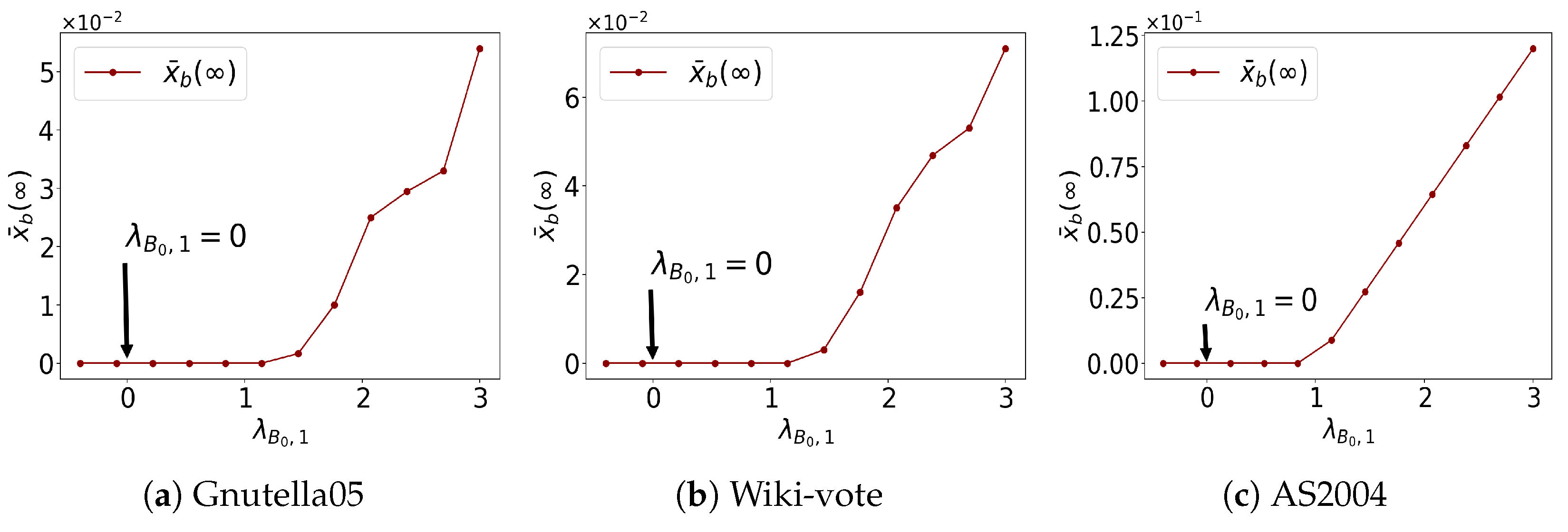
• Gnutella05 peer-to-peer network: This is a directed graph, representing a peer-to-peer (P2P) network. It has 8846 nodes, 31,839 arcs, and its adjacency matrix has the largest eigenvalue of ${\lambda }_{A,1}=4.36$. It is not strongly connected.
• Wiki-vote network: The directed network contains all the Wikipedia voting data from the inception of Wikipedia till January 2008. It has 7115 nodes, 103,689 arcs, and its adjacency matrix has the largest eigenvalue of ${\lambda }_{A,1}=45.14$. It is not strongly connected.
• AS-CAIDA (Cooperative Association for Internet Data Analysis) 2004 network: It is a directed network derived from a set of RouteViews BGP table snapshots. It has 16,301 nodes, 65,910 arcs, and its adjacency matrix has the largest eigenvalue of ${\lambda }_{A,1}=62.56$. It is strongly connected.

5.1.2. Setting Model Parameters

We consider a system with three good states and three states, namely $\mathcal{G}=\{1,2,3\}$ and $\mathcal{B}=\{-1,-2,-3\}$. As the theoretical analysis and the three operations are independent of the good-to-good transitions, we set $p_{v,i,i^{\prime }}=0.1$, for $v\in V$ and $i,i^{\prime }\in \mathcal{G}$ for simplicity, and the setting satisfies the condition for Lemma 5, that is, $\mathcal{N}$ has a unique fixed point $x^{*}$. The condition probability that type 1 bad-to-bad transition happens ${\delta }_{v,i}$ is set as ${\displaystyle \frac{1}{2}}$ as there is no real data to indicate what the value is.

Due to excessive parameters, for the sake of convenience in representation and to appropriately simplify the calculations, we set the following: (1) for each node v, the bad-to-good transition rate $p_{v,j,i}$ for $j\in \mathcal{B}$ and $i\in \mathcal{G}$ is sampled from $U([0,2{\overline{p}}_{bg}])$, the uniform distribution on $[0,2{\overline{p}}_{bg}]$; (2) the type 1 bad-to-bad transition rate $p_{v,j,j^{\prime }}$, $j,j^{\prime }\in \mathcal{B}$ are sampled from $U([0,2{\overline{p}}_{bb}])$; (3) the type 2 bad-to-bad infection rate ${\gamma }_{u,v}^{(j^{\prime },l,j)}$ are sampled from $U([0,2{\overline{\gamma }}_{bb}])$; and (4) the type 2 good-to-bad infection rate ${\gamma }_{u,v}^{(i,l,j)}$ are sampled from $U([0,2{\overline{\gamma }}_{gb}])$, where ${\overline{p}}_{bg}$, ${\overline{p}}_{bb}$, ${\overline{\gamma }}_{bb}$, and ${\overline{\gamma }}_{gb}$ are parameters to be determined. This setting makes the parameters of our model heterogeneous while facilitating control.

5.1.3. Simulation Method

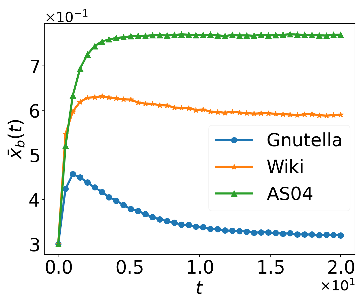
We employ the method from [37] to bridge the gap between the probabilistic states in System (2) (the probabilities of nodes being in various states at a given moment) and the discrete states in reality (a node can only be in one state at a given moment). After setting the initial values and parameters, we solve System (2) using the Euler method with a step size of 0.01. At time t, for node $v\in V$, obtain the probabilities of it being in each state: $(x_{v,3}(t),x_{v,2}(t),x_{v,1}(t),x_{v,-1}(t),x_{v,-2}(t),x_{v,-3}(t))$. At time t, the simulated state of node v, ${\xi }_v(t)$, is sampled from a random variable with values $(3,2,1,-1,-2,-3)$ and probabilities corresponding to the aforementioned probability sequence.

For the sake of numerical simulation, we set ${\theta }_{v,i,j}(t)$ to be the ∑-model, that is, we set $R_{i,j}^v=0$ in Equation (3) which is the same as [3].

For the initial infection state, we randomly select nodes according to the initial infection rate $p_0$. If a node v is selected, it is assigned a bad state $j\in \mathcal{B}$ randomly, that is, $x_{v,j}(0)=1$; if node v is not selected, it is assigned a good state $i\in \mathcal{G}$ randomly, that is, $x_{v,i}(0)=1$, which is the same as [20].

We let ${\overline{x}}_b(t)={\displaystyle \frac{1}{k}}{\displaystyle \sum _{v\in V}}{\mathbb{1}}_{{\xi }_v\in \mathcal{B}}$ to be the fraction of nodes in the network that are in bad states at time t, and let ${\overline{x}}_b(\infty )={\displaystyle \underset{t\in \infty }{lim}}{\overline{x}}_b(t)$ to be the fraction of nodes in the network that are in bad states at steady state. In the numerical simulation, ${\overline{x}}_b(\infty )$ is taken as the average value of ${\overline{x}}_b(t)$ over the time interval from $t=280$ to $t=300$.

5.2. Confirming $x^{*}$’s Global Asymptotic Stability (Theorem 1)

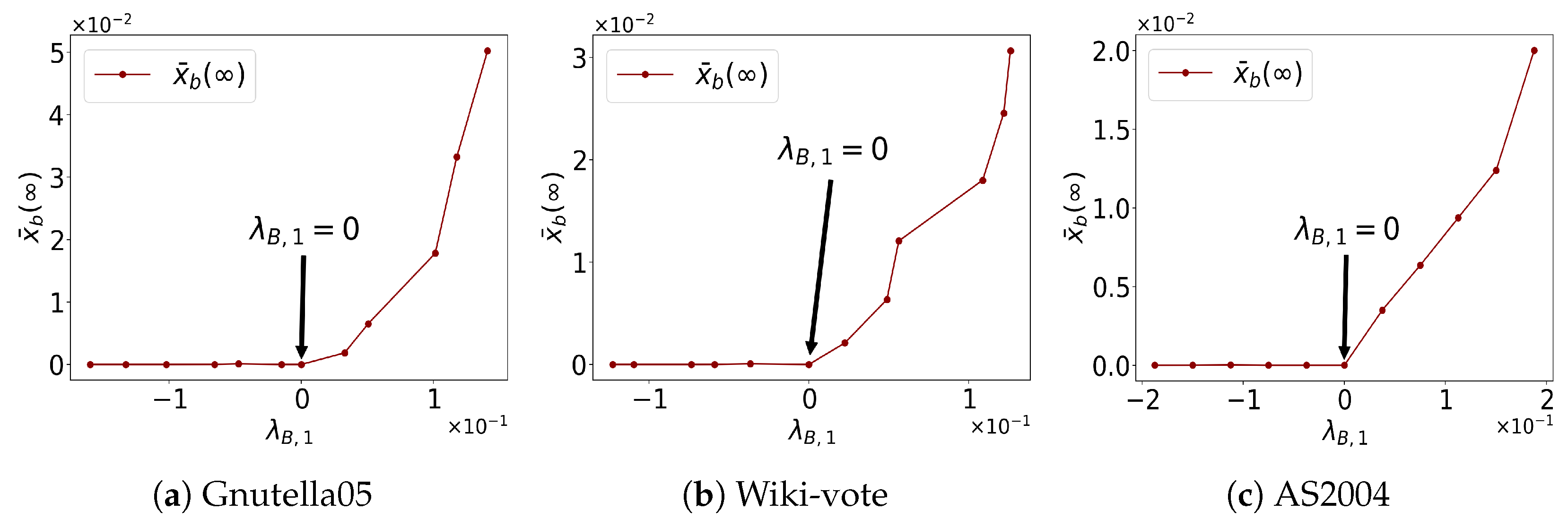
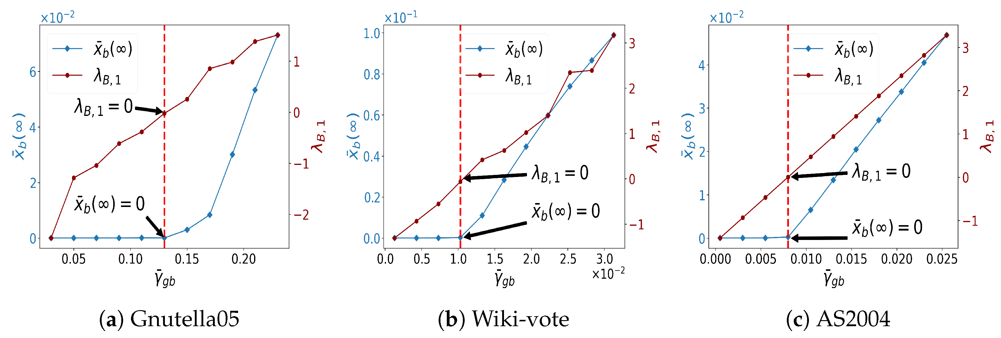
To verify the $x^{*}$’s (Theorem 1) global asymptotic stability, we set $p_0=0.85$. Figure 2 illustrates the impact of the variation in ${\lambda }_{B_0,1}$ in the three networks on the proportion of nodes in the bad states when the system reaches a steady state (denoted as ${\overline{x}}_b(\infty )$), as carried out in the experiment in [19].

It can be observed that even if the initial infection situation is very severe, with $85\%$ of the nodes being initially infected, when ${\lambda }_{B_0,1}<0$, ${\overline{x}}_b(\infty )=0$. This indicates that the bad state is eradicated as the system evolves, which confirms Theorem 1. At the same time, when ${\lambda }_{B_0,1}>0$, the bad state will also be eradicated. This suggests that ${\lambda }_{B_0,1}<0$ is a sufficient condition for the global asymptotic stability of $x^{*}$, but not a necessary condition.

We have placed the source code for the experimental section in a GitHub repository. The experiments were conducted using Python version 3.8.3. Here is the link to the repository: https://github.com/Yonion2/transdiagram/ (accessed on 12 June 2025).

5.3. Confirming $x^{*}$’s Locally Asymptotic Stability (Theorem 2)

The local asymptotic stability of $x^{*}$ is a generalization of the epidemic threshold condition. We set the initial infection rate $p_0=0.0375$, the same as [18]. Figure 3 illustrates the impact of the variation in ${\lambda }_{B,1}$ in the three networks on the proportion of nodes in the bad states when the system reaches a steady state (denoted as ${\overline{x}}_b(\infty )$).

It can be observed that ${\lambda }_{B,1}=0$ acts as a threshold: when ${\lambda }_{B,1}<0$, all bad states disappear, and when ${\lambda }_{B,1}>0$, bad states are preserved in the system.

5.4. Sensitivity Analysis Regarding ${\overline{\gamma }}_{gb}$ and ${\overline{p}}_{bg}$

To investigate the impact of parameter variations on ${\lambda }_{B,1}$ and ${\overline{x}}_b(\infty )$, and to better reflect that ${\lambda }_{B,1}=0$ is a critical threshold condition, we seek parameter combinations that place ${\lambda }_{B,1}$ near zero. We then perturb ${\overline{p}}_{bg}$ and ${\overline{\gamma }}_{gb}$ separately, and analyze the sensitivity of ${\lambda }_{B,1}$ and ${\overline{x}}_b(\infty )$ to ${\overline{p}}_{bg}$ and ${\overline{\gamma }}_{gb}$. To eliminate the randomness in the experiments and focus on the impact of parameters on ${\lambda }_{B,1}$ and ${\overline{x}}_b(\infty )$.

Consider the following initial parameters: On Gnutella05 network, set $({\overline{\gamma }}_{gb},{\overline{\gamma }}_{bb},{\overline{p}}_{bb},{\overline{p}}_{bg})=(0.13,0.1,0.1,0.7)$; on Wiki-vote network $({\overline{\gamma }}_{gb},{\overline{\gamma }}_{bb},{\overline{p}}_{bb},{\overline{p}}_{bg})=(0.011,0.1,0.1,0.5)$; and on and AS2004 network $({\overline{\gamma }}_{gb},{\overline{\gamma }}_{bb},{\overline{p}}_{bb},{\overline{p}}_{bg})=(0.01,0.1,0.1,0.5)$. Under the aforementioned parameter combinations, ${\lambda }_{B,1}$ is close to 0.

First we focus on the impact of the perturbation of ${\overline{p}}_{bg}$ on ${\lambda }_{B,1}$ and ${\overline{x}}_b(\infty )$. Keeping the other parameters constant, we let ${\overline{p}}_{bg}$ take 11 evenly spaced values in the interval $[0,1]$. Figure 4 illustrates the variation in ${\lambda }_{B,1}$ and ${\overline{x}}_b(\infty )$ with ${\overline{p}}_{bg}$ for each network. Because ${\lambda }_{B,1}$ and ${\overline{x}}_b(\infty )$ are of different orders of magnitude, we use the left blue y-axis to represent the values of ${\overline{x}}_b(\infty )$ and the right dark red y-axis to represent the values of ${\lambda }_{B,1}$. The values of ${\overline{x}}_b(\infty )$ are indicated by a blue curve, while the values of ${\lambda }_{B,1}$ are indicated by a dark red curve. The initial position of ${\overline{p}}_{bg}$ is marked with a red dashed line, and the positions where ${\lambda }_{B,1}=0$ and ${\overline{x}}_b(\infty )=0$ are indicated by black arrows.

Then, we focus on the impact of the variation in ${\gamma }_{gb}$ on ${\lambda }_{B,1}$ and ${\overline{x}}_b(\infty )$. For the initial parameters, we fix ${\overline{p}}_{bb}$, ${\overline{p}}_{bg}$, and ${\overline{\gamma }}_{bb}$, and perturb ${\overline{\gamma }}_{gb}$. Figure 5 illustrates ${\lambda }_{B,1}$ and ${\overline{x}}_b(\infty )$ under different values of ${\overline{\gamma }}_{gb}$, with the content of the plot being similar to that described earlier.

As can be seen from Figure 4 and Figure 5, regardless of whether ${\overline{p}}_{bg}$ or ${\overline{\gamma }}_{gb}$ is perturbed, when ${\lambda }_{B,1}<0$, ${\overline{x}}_b(\infty )=0$; and when ${\lambda }_{B,1}>0$, ${\overline{x}}_b(\infty )>0$. This further validates the criticality of the condition ${\lambda }_{B,1}=0$, as stated in Theorem 2. Moreover, increasing ${\overline{p}}_{bg}$ monotonically decreases ${\lambda }_{B,1}$, while increasing ${\overline{\gamma }}_{gb}$ monotonically increases ${\lambda }_{B,1}$. This confirms the effects of Operation 1 and Operation 2.

5.5. Confirming Persistence of Bad States (Theorems 3)

Since we set ${\theta }_{v,i,j}(t)$ as the ∑-model in the numerical experiments, verifying Theorem 3 is transformed into verifying Corollary 4. For the sake of computational convenience, for $i\in \mathcal{G}$ and $l,j\in \mathcal{B}$, we set $p_{v,j,i}=0.1$, ${\gamma }_{u,v}^{(i,l,j)}=0.2$, and $b=0.3$. This set of parameters can be verified to satisfy the conditions in the corollary. Then we set $p_0=b=0.3$, ${\overline{\gamma }}_{bb}=0.1={\overline{p}}_{bb}=0.1$. Figure 6 illustrates the trend of the proportion of nodes in the bad state ${\overline{x}}_b(t)$ over time for the three networks under the aforementioned parameters. It can be observed that our model exhibits distinct dynamical behaviors across the three networks. However, the proportion of nodes in the bad state always remains above $0.3$, which validates Theorem 3.

Remark 3.

When ${\lambda }_{B,1}>0$, the model exhibits complex dynamical behavior. The proportion of nodes in the bad state may monotonically tend to a fixed point, as demonstrated on the AS04 network, or it may first increase and then decrease, as observed in the Gnutella05 network. We can only provide a sufficient condition for the existence of a non-zero fixed point for the bad state. The necessary conditions for its existence and the specific values still need further investigation.

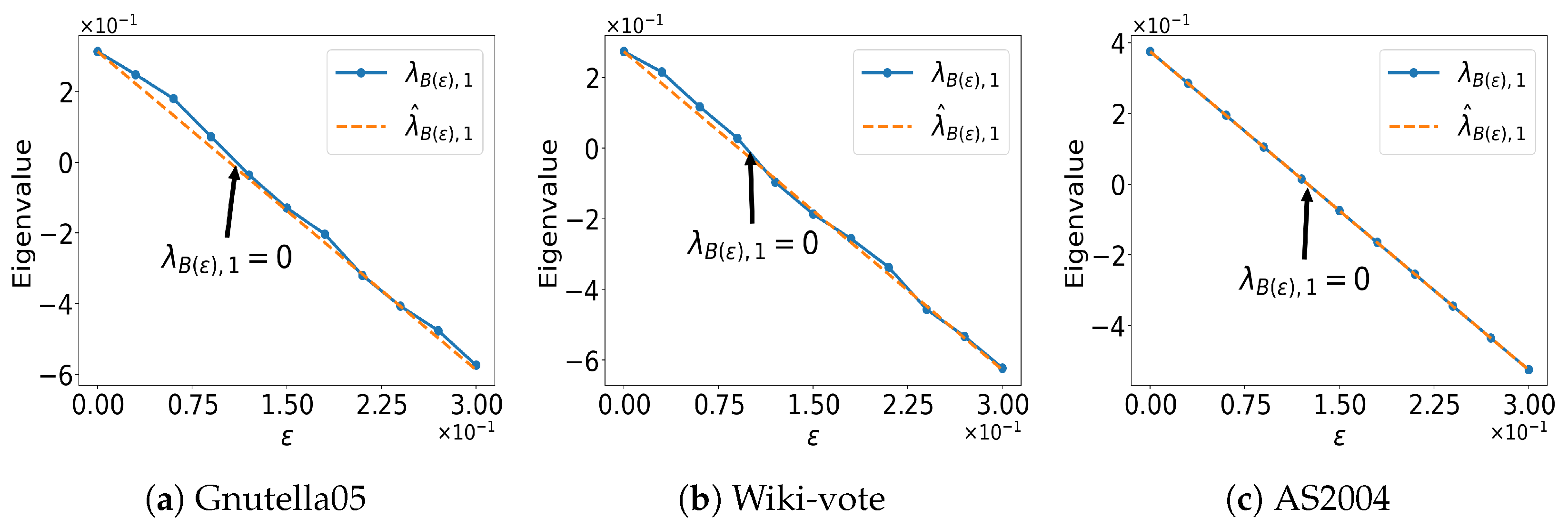
5.6. Confirming Practical Guidance (Theorems 4)

It can be observed from the experiment above that even if it is not possible to achieve ${\lambda }_{B_0,1}<0$ or ${\lambda }_{B,1}<0$, reducing their values still helps in controlling the evolution of the virus. In this subsection, we will use experiments to verify that the three operations we proposed can indeed reduce ${\lambda }_{B_0,1}$ and ${\lambda }_{B,1}$: Operation 1 increase ${\overline{p}}_{bg}$, Operation 2 decrease ${\overline{\gamma }}_{gb}$, and Operation 3 add a new state that cannot infect nodes in good states.

Because the three operations have similar effects on ${\lambda }_{B_0,1}$ and ${\lambda }_{B,1}$, we only investigate their impact on ${\lambda }_{B,1}$. For the sake of convenience in control, we assume the model parameters to be homogeneous, i.e., for $i\in \mathcal{G}$ and $j,j^{\prime },l\in \mathcal{B}$, ${\gamma }_{u,v}^{(i,l,j)}={\overline{\gamma }}_{gb}$, ${\gamma }_{u,v}^{(j^{\prime },l,j)}={\overline{\gamma }}_{bb}$,$p_{v,j,i}={\overline{p}}_{bg}$, and $p_{v,j,j^{\prime }}={\overline{p}}_{bb}$.

As shown in the proof of Theorem 4, the effect of an operation with perturbation strength $\epsilon$ on ${\lambda }_{B,1}$ can be estimated by a linear function of $\epsilon$. Let $B(\epsilon )$ denote the matrix B perturbed by an operation of strength $\epsilon$, ${\lambda }_{B(\epsilon ),1}$ is its largest eigenvalue, and ${\widehat{\lambda }}_{B(\epsilon ),1}$ is our estimate of it. We would like to verify the accuracy of this estimate.

5.6.1. Confirming Operation 1

We set ${\overline{p}}_{bg}=0$ and Operation 1 with strength $\epsilon$ makes ${\overline{p}}_{bg}=\epsilon$. On Gnutella05 network, set $({\overline{\gamma }}_{gb},{\overline{\gamma }}_{bb},{\overline{p}}_{bb})=(0.02,0.1,0.1)$ and on Wiki-vote network and AS2004 network, $({\overline{\gamma }}_{gb},{\overline{\gamma }}_{bb},{\overline{p}}_{bb})=(0.002,0.1,0.1)$.

Figure 7 illustrates the changes in ${\lambda }_{B(\epsilon ),1}$ and our estimate ${\widehat{\lambda }}_{B(\epsilon ),1}$ as $\epsilon$ increases. It can be observed that Operation 1 indeed reduces ${\lambda }_{B,1}$, and the magnitude of the reduction is consistent with our estimate.

Remark 4.

Operation 1 increases the rate at which nodes recover from bad states. For instance, in the field of epidemiology, it is akin to providing a specific medication during an H1N1 influenza outbreak. In the realm of cybersecurity, it involves adopting a reactive defense strategy against computer viruses: targeting the Persistence tactic within the MITRE ATT&CK framework, monitoring execution commands and parameters that could configure system settings, as well as unusual kernel driver installation activities that might be used to set up system configurations. This reduces the likelihood of viruses persisting long-term within computers, allowing them to return to a normal state.

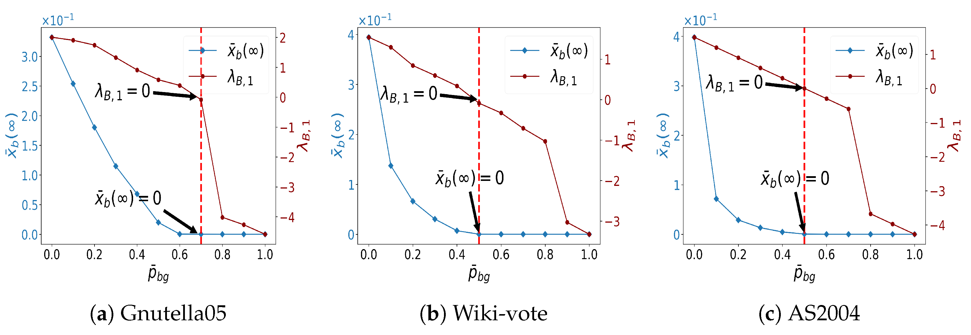
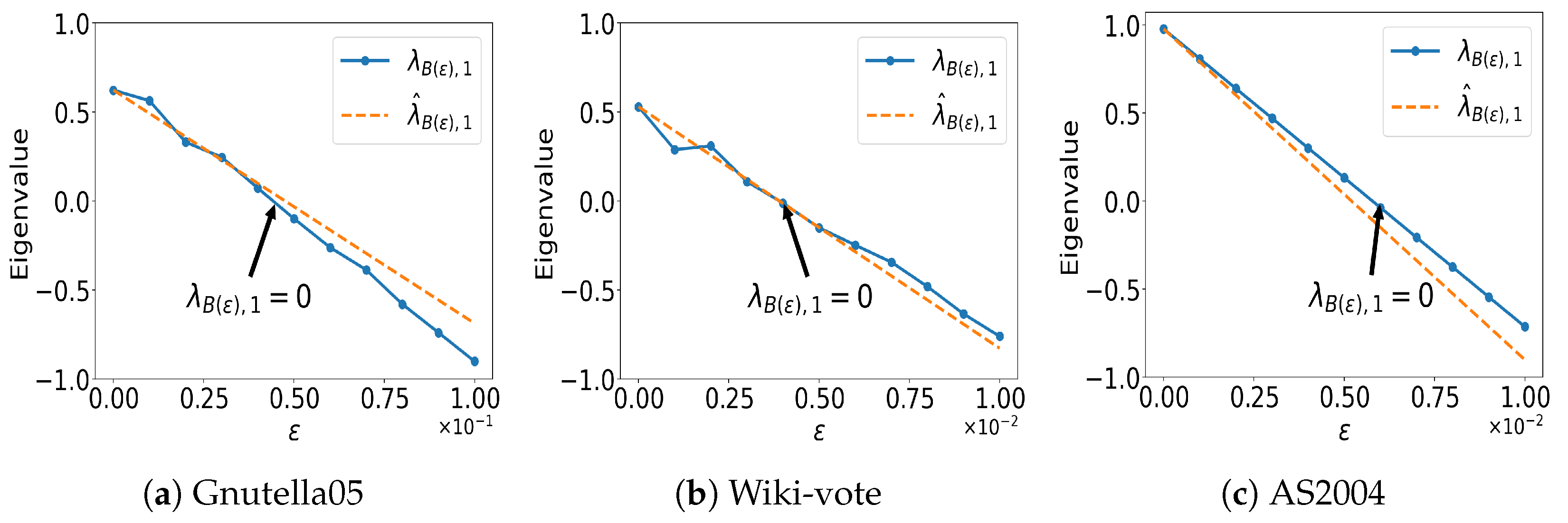
5.6.2. Confirming Operation 2

Operation 2 with strength $\epsilon$ decrease ${\overline{\gamma }}_{gb}$ by $\epsilon$. On Gnutella05 network, set $({\overline{p}}_{bg},{\overline{\gamma }}_{gb},{\overline{\gamma }}_{bb},{\overline{p}}_{bb})=(0.3,0.1,0.1,0.1)$ and on Wiki-vote network and AS2004 network, $({\overline{p}}_{bg},{\overline{\gamma }}_{gb},{\overline{\gamma }}_{bb},{\overline{p}}_{bb})=(0.3,0.01,0.1,0.1)$. Figure 8 plots the change in ${\lambda }_{B(\epsilon ),1}$ and ${\widehat{\lambda }}_{B(\epsilon ),1}$ as $\epsilon$ increases. Operation 2 indeed reduces ${\lambda }_{B,1}$, and our estimate is quite accurate when $\epsilon$ is small.

Remark 5.

Operation 2 reduces the virus’s ability to infect. For instance, in the field of epidemiology, vaccinating the entire population enhances the community’s resistance to the virus. In the field of cybersecurity, employing a preventive defense strategy involves targeting the “Initial Access” and “Lateral Movement” tactics within the MITRE ATT&CK framework. This includes using firewalls and proxies to inspect URLs for potential known malicious domains or parameters, monitoring newly created files written to disk, watching for unexpected network share access, and observing unusual processes that create system files over internal network connections.

5.6.3. Confirming Operation 3

Operation 3 introduces a new state, -4, that does not infect good-state nodes and it will not be infected by other bad states, i.e., ${\gamma }_{u,v}^{(i,\text{-}4,j)}=p_{v,\text{-}4,j}={\gamma }_{u,v}^{(\text{-}4,l,j)}=0$, and the strength $\epsilon$ representing $p_{v,j,\text{-}4}=p_{v,\text{-}4,i}={\gamma }^{j^{\prime },\text{-}4,j}=\epsilon$, for $i\in \mathcal{G}$ and $j,j^{\prime },l\in \mathcal{B}$. On the Gnutella05 network, $({\overline{p}}_{bg},{\overline{\gamma }}_{gb},{\overline{\gamma }}_{bb},{\overline{p}}_{bb})=(0.1,0.1,0.1,0.04)$ and on the Wiki-vote network and AS2004 network, $({\overline{p}}_{bg},{\overline{\gamma }}_{gb},{\overline{\gamma }}_{bb},{\overline{p}}_{bb})=(0.1,0.1,0.1,0.004)$.

Figure 9 plots the change in ${\lambda }_{B(\epsilon ),1}$ and ${\widehat{\lambda }}_{B(\epsilon ),1}$ as $\epsilon$ increases. It is evident that ${\lambda }_{B,1}$ indeed decreases with the increase in $\epsilon$, and our estimate accurately predicts the downward trend.

Remark 6.

Operation 3 corresponds to the active defense strategy in cybersecurity. For example, the “replicative patching” strategy mentioned in the literature [36], allowing antivirus software and patches to spread through the network like a virus, automatically seeking out infected nodes and completing the repair.

6. Conclusions and Discussion

6.1. Our Contibutions

In this paper, we have presented a generalized multistate complex network contagion dynamics model with respect to arbitrary networks and showed that our model and results can supersede four models and their results in the literature by accommodating them as special cases, including both cybersecurity dynamics models and other models. Researchers can, under this unified theoretical framework, more efficiently explore the complex interactions between different network structures, propagation mechanisms, and individual behaviors, thereby providing more universal theoretical support for solving practical issues such as information diffusion, public opinion guidance, and the spread of computer viruses.

We characterized the newly proposed dynamics, including the following: a sufficient condition under which the dynamics are globally asymptotically stable; a sufficient condition under which the dynamics are locally asymptotically stable; and a sufficient condition for the persistence of the bad states. We further proposed three operations on the transition diagram to make the following dynamics manageable: (i) increasing the bad-to-good transition rate $p_{v,i,j}$; (ii) decreasing the good-to-bad transition rate ${\gamma }_{u,v}^{i,l,j}$; (iii) adding a white bad state, which grabs nodes in the bad states but does not attack nodes in good states. These three operations can be regarded as three defensive strategies in the field of cybersecurity: reactive defense, preventive defense, and active defense (deploying the replicative patches [36]).

6.2. Limitations and Future Work

Our research has certain limitations: Firstly, our model is a theoretical framework primarily designed to explore the impact of network structure on dynamic behaviors. Applying it to practical situations presents several challenges, such as significantly increased computational complexity when the network has a large number of nodes. Additionally, obtaining model parameters in real-world applications is quite difficult, as infection rates for diseases or computer viruses are hard to measure directly, and there may be numerous errors in the underlying network structure information. Secondly, the lack of real-world data to validate the model’s effectiveness is a concern. Currently, datasets related to contagion dynamics generally lack information on network structures, so the verification of conclusions drawn from complex network contagion models often relies on synthetic data, which results in a weaker connection between the model and real-world scenarios.

Our future work will focus on two main aspects:

• Construction of real (simulated) datasets for complex network contagion dynamics: We aim to collect real datasets that contain both dynamic information and underlying network structure, or to construct similar datasets through simulation experiments, such as using virtual machines to simulate the process of computer virus attacks on computer clusters to obtain relevant data. By building these datasets, we can closely integrate the theory of complex network epidemic dynamics with real scenarios, making the corresponding theories more convincing.
• Seeking more efficient modeling methods: To study the impact of network structure on dynamics, the current approach is to explicitly incorporate network structure into the model, which is a common method used in academia. However, this modeling approach results in high model dimensions and significantly increased computational complexity, making it difficult to predict future dynamic behaviors and other practical scenarios. Therefore, it is necessary to find a modeling method that can reflect the influence of network structure while also being solvable quickly.

References

1. Epstein, J.M.; Parker, J.; Cummings, D.; Hammond, R.A. Coupled contagion dynamics of fear and disease: Mathematical and computational explorations. PLoS ONE 2008, 3, e3955. [Google Scholar] [CrossRef] [PubMed]
2. Wang, Y.; Chakrabarti, D.; Wang, C.; Faloutsos, C. Epidemic spreading in real networks: An eigenvalue viewpoint. In Proceedings of the 22nd International Symposium on Reliable Distributed Systems, Florence, Italy, 6–8 October 2003; pp. 25–34. [Google Scholar] [CrossRef]
3. Lin, Z.; Lu, W.; Xu, S. Unified Preventive and Reactive Cyber Defense Dynamics Is Still Globally Convergent. IEEE/ACM ToN 2019, 27, 1098–1111. [Google Scholar] [CrossRef]
4. Han, Y.; Lu, W.; Xu, S. Preventive and Reactive Cyber Defense Dynamics with Ergodic Time-dependent Parameters Is Globally Attractive. IEEE TNSE 2021, 8, 2517–2532. [Google Scholar] [CrossRef]
5. Zheng, R.; Lu, W.; Xu, S. Active Cyber Defense Dynamics Exhibiting Rich Phenomena. In Proceedings of the 2015 Symposium and Bootcamp on the Science of Security, Urbana, IL, USA, 21–22 April 2015. [Google Scholar]
6. Xu, S.; Lu, W.; Li, H. A Stochastic Model of Active Cyber Defense Dynamics. Internet Math. 2015, 11, 23–61. [Google Scholar] [CrossRef]
7. Anderson, R.M.; May, R.M. Infectious Diseases of Humans: Dynamics and Control; Oxford University Press: Oxford, UK, 1991. [Google Scholar]
8. Zhang, J.; Moura, J.M. Diffusion in social networks as SIS epidemics: Beyond full mixing and complete graphs. IEEE J. Sel. Top. Signal Process. 2014, 8, 537–551. [Google Scholar] [CrossRef]
9. She, B.; Liu, J.; Sundaram, S.; Paré, P.E. On a networked SIS epidemic model with cooperative and antagonistic opinion dynamics. IEEE Trans. Control. Netw. Syst. 2022, 9, 1154–1165. [Google Scholar] [CrossRef]
10. Huang, J.; Ma, X.; Wu, H.; Awuxi, H.; Zhang, X.; Chen, Y.; Alitengsaier, N.; Li, Q. Retrospective study on the epidemiological characteristics of multi-pathogen infections of hospitalized severe acute respiratory tract infection and influenza-like illness in Xinjiang from January to May 2024. BMC Infect. Dis. 2025, 25, 252. [Google Scholar] [CrossRef]
11. Akhtar, Z.B. Securing operating systems (OS): A comprehensive approach to security with best practices and techniques. Int. J. Adv. Network, Monit. Control. 2024, 9, 100–111. [Google Scholar] [CrossRef]
12. Bontchev, V. Possible macro virus attacks and how to prevent them. Comput. Secur. 1996, 15, 595–626. [Google Scholar] [CrossRef]
13. Pawar, M.V.; Anuradha, J. Network security and types of attacks in network. Procedia Comput. Sci. 2015, 48, 503–506. [Google Scholar] [CrossRef]
14. Cremer, F.; Sheehan, B.; Fortmann, M.; Kia, A.N.; Mullins, M.; Murphy, F.; Materne, S. Cyber risk and cybersecurity: A systematic review of data availability. Geneva Pap. Risk Insur. Issues Pract. 2022, 47, 698. [Google Scholar] [CrossRef]
15. Li, M.Y.; Muldowney, J.S. Global stability for the SEIR model in epidemiology. Math. Biosci. 1995, 125, 155–164. [Google Scholar] [CrossRef] [PubMed]
16. Paré, P.E.; Vrabac, D.; Sandberg, H.; Johansson, K.H. Analysis, Online Estimation, and Validation of a Competing Virus Model. In Proceedings of the 2020 American Control Conference (ACC), Denver, CO, USA, 1–3 July 2020; pp. 2556–2561. [Google Scholar] [CrossRef]
17. Basnarkov, L. SEAIR Epidemic spreading model of COVID-19. Chaos Solitons Fractals 2021, 142, 110394. [Google Scholar] [CrossRef] [PubMed]
18. Xu, S.; Lu, W.; Zhan, Z. A Stochastic Model of Multivirus Dynamics. IEEE Trans. Dependable Secur. Comput. 2012, 9, 30–45. [Google Scholar] [CrossRef]
19. Prakash, B.A.; Chakrabarti, D.; Faloutsos, M.; Valler, N.; Faloutsos, C. Threshold Conditions for Arbitrary Cascade Models on Arbitrary Networks. In Proceedings of the 2011 IEEE 11th International Conference on Data Mining, Vancouver, BC, Canada, 11–14 December 2011; pp. 537–546. [Google Scholar] [CrossRef]
20. Sahneh, F.D.; Scoglio, C.; Van Mieghem, P. Generalized epidemic mean-field model for spreading processes over multilayer complex networks. IEEE/ACM Trans. Netw. 2013, 21, 1609–1620. [Google Scholar] [CrossRef]
21. Brandon, J. Introduction to applied nonlinear dynamical systems and chaos, by S Wiggins. Pp 672. DM98.00. 1990. ISBN 3-540-9703-7 (Springer). Math. Gaz. 1991, 75, 255. [Google Scholar] [CrossRef]
22. Green, S.L. Ordinary Differential Equations. By Jack K. Hale. Pp. xvi, 332. 1969. (Wiley-Interscience). Math. Gaz. 1971, 55, 485–486. [Google Scholar] [CrossRef]
23. Gray, A.; Greenhalgh, D.; Hu, L.; Mao, X.; Pan, J. A stochastic differential equation SIS epidemic model. SIAM J. Appl. Math. 2011, 71, 876–902. [Google Scholar] [CrossRef]
24. Zheng, R.; Lu, W.; Xu, S. Preventive and Reactive Cyber Defense Dynamics Is Globally Stable. IEEE TNSE 2018, 5, 156–170. [Google Scholar] [CrossRef]
25. Persoons, R.; Van Mieghem, P. Finding patient zero in susceptible-infectious-susceptible epidemic processes. Phys. Rev. E 2024, 110, 044308. [Google Scholar] [CrossRef]
26. Chakrabarti, D.; Wang, Y.; Wang, C.; Leskovec, J.; Faloutsos, C. Epidemic thresholds in real networks. ACM Trans. Inf. Syst. Secur. 2008, 10, 1–26. [Google Scholar] [CrossRef]
27. Van Mieghem, P.; Omic, J.; Kooij, R. Virus Spread in Networks. IEEE/ACM Trans. Netw. 2009, 17, 1–14. [Google Scholar] [CrossRef]
28. Mieghem, P.V. The N-intertwined SIS epidemic network model. Computing 2011, 93, 147–169. [Google Scholar] [CrossRef]
29. Xu, S.; Lu, W.; Xu, L. Push- and pull-based epidemic spreading in networks: Thresholds and deeper insights. ACM TAAS 2012, 7, 1–26. [Google Scholar] [CrossRef]
30. Xu, S. The Cybersecurity Dynamics Way of Thinking and Landscape (invited paper). In Proceedings of the ACM Workshop on Moving Target Defense, Los Angeles, CA, USA, 7 November 2022. [Google Scholar]
31. Paré, P.E.; Liu, J.; Beck, C.L.; Nedić, A.; Başar, T. Multi-competitive viruses over time-varying networks with mutations and human awareness. Automatica 2021, 123, 109330. [Google Scholar] [CrossRef]
32. Chakrabarti, D.; Leskovec, J.; Faloutsos, C.; Madden, S.; Guestrin, C.; Faloutsos, M. Information Survival Threshold in Sensor and P2P Networks. In Proceedings of the IEEE INFOCOM 2007—26th IEEE International Conference on Computer Communications, Anchorage, AK, USA, 6–12 May 2007; pp. 1316–1324. [Google Scholar] [CrossRef]
33. Ashwin, P.; Buescu, J.; Stewart, I.N. From attractor to chaotic saddle: A tale of transverse instability. Nonlinearity 1996, 9, 703–737. [Google Scholar] [CrossRef]
34. Strom, B.E.; Applebaum, A.; Miller, D.P.; Nickels, K.C.; Pennington, A.G.; Thomas, C.B. Mitre Att&CK: Design and Philosophy; Technical Report; The MITRE Corporation: McLean, VA, USA, 2018. [Google Scholar]
35. Carlton, M.; Levy, Y. Cybersecurity skills: Foundational theory and the cornerstone of advanced persistent threats (APTs) mitigation. Online J. Appl. Knowl. Manag. (OJAKM) 2017, 5, 16–28. [Google Scholar] [CrossRef]
36. Eshghi, S.; Khouzani, M.; Sarkar, S.; Venkatesh, S.S. Optimal patching in clustered epidemics of malware. IEEE Trans. Netw. 2015, 24, 283–298. [Google Scholar] [CrossRef]
37. Liu, Z.; Zheng, R.; Lu, W.; Xu, S. Using event-based method to estimate cybersecurity equilibrium. IEEE/CAA J. Autom. Sin. 2020, 8, 455–467. [Google Scholar] [CrossRef]
38. Horn, R.A.; Johnson, C.R. Matrix Analysis, 2nd ed.; Cambridge University Press: Cambridge, UK, 2012. [Google Scholar]
39. Milanese, A.; Sun, J.; Nishikawa, T. Approximating spectral impact of structural perturbations in large networks. Phys. Rev. E 2010, 81, 046112. [Google Scholar] [CrossRef]
40. Mitchell, A.R. J. H. Wilkinson, The Algebraic Eigenvalue Problem (Clarendon Press, Oxford, 1965), 662pp., 110s. Proc. Edinb. Math. Soc. 1967, 15, 328. [Google Scholar] [CrossRef]
41. Shilnikov, L.P.; Shilnikov, A.L.; Turaev, D.V.; Chua, L.O. Methods of Qualitative Theory in Nonlinear Dynamics: (Part II); World Scientific: Singapore, 2001. [Google Scholar]
42. Kellogg, R.B.; Li, T.Y.; Yorke, J. A Constructive Proof of the Brouwer Fixed-Point Theorem and Computational Results. SIAM J. Numer. Anal. 1976, 13, 473–483. [Google Scholar] [CrossRef]
Figure 1. The state transition diagram of a model with two good states and two bad states, where θ v , i , j ( t ) represents neighbor-dependent transitions.
Axioms 14 00487 g001
Figure 2. The change in x ¯ b ( ) with respect to λ B 0 , 1 .
Axioms 14 00487 g002
Figure 3. The change in x ¯ b ( ) with respect to λ B , 1 .
Axioms 14 00487 g003
Figure 4. The impact of perturbation in p ¯ b g on λ B , 1 and x ¯ b ( ) .
Axioms 14 00487 g004
Figure 5. The impact of perturbation in γ ¯ g b on λ B , 1 and x ¯ b ( ) .
Axioms 14 00487 g005
Figure 6. Persistence of bad states and the results are obtained by averaging over 50 Monte Carlo samples.
Axioms 14 00487 g006
Figure 7. The effect of Operation 1 on λ B , 1 .
Axioms 14 00487 g007
Figure 8. The effect of Operation 2 on λ B , 1 .
Axioms 14 00487 g008
Figure 9. The effect of Operation 3 on λ B , 1 .
Axioms 14 00487 g009