Article

Bayesian Quantile Regression for Partial Functional Linear Spatial Autoregressive Model

1
School of Economics, Hangzhou Dianzi University, Hangzhou 310018, China
2
School of Mathematics, Hangzhou Normal University, Hangzhou 311121, China
*
Author to whom correspondence should be addressed.
Axioms 2025, 14(6), 467; https://doi.org/10.3390/axioms14060467
Submission received: 6 April 2025 / Revised: 8 June 2025 / Accepted: 13 June 2025 / Published: 16 June 2025

Abstract

:
When performing Bayesian modeling on functional data, the assumption of normality is often made on the model error and thus the results may be sensitive to outliers and/or heavy tailed data. An important and good choice for solving such problems is quantile regression. Therefore, this paper introduces the quantile regression into the partial functional linear spatial autoregressive model (PFLSAM) based on the asymmetric Laplace distribution for the errors. Then, the idea of the functional principal component analysis, and the hybrid MCMC algorithm combining Gibbs sampling and the Metropolis–Hastings algorithm are developed to generate posterior samples from the full posterior distributions to obtain Bayesian estimation of unknown parameters and functional coefficients in the model. Finally, some simulation studies show that the proposed Bayesian estimation method is feasible and effective.

1. Introduction

With the rapid development of data collection and storage technology, people often obtain a kind of data that appears in the form of curves, surfaces or more complex structures. This type of data with obvious functional characteristics is called functional data, which widely exist in stock data, electrocardiogram data, weather data, spectral data, etc. Over the last two decades, functional data analysis is becoming an useful tool to deal with this type of data and has received increasing attention in fields such as econometrics, meteorology, biomedical research, chemometrics, as well as other applied fields. Therefore, there has been a large amount of work in function data analysis and various functional regression models have also been proposed one after another; see [1,2,3,4], among others. However, the collected data may contain both functional covariates and scalar covariates, so classical functional linear regression models are no longer sufficient for research needs. Subsequently, some methods and theories on the partial functional linear model (PFLM) have been introduced. For example, Shin [5] proposed new estimators of partial functional linear model and established its asymptotical normality. Cui et al. [6] investigated a partially functional linear regression model based on reproducing kernel Hilbert spaces. Xiao et al. [7] studied the partial functional linear model with autoregressive errors. Li et al. [8] applied partially functional linear regression models for analysis of genetic, imaging, and clinical data. It can be observed that the above studies focus on mean regression, which typically assume the normality of error and are very sensitive to heavy-tailed distributions or outliers. As a feasible alternative, quantile regression (QR), first proposed by Koenker and Bassett [9], not only can provide a more complete statistical analysis of the relationship between the conditional quantiles of explanatory variables and response variables than mean regression, but is also more robust, and has received widespread attention. When dealing with infinite dimensional data such as functional data, many scholars have already combined quantile regression with functional data analysis and conducted research on related theories and applications. For example, Yang et al. [10] studied functional quantile linear regression within the framework of reproducing kernel Hilbert spaces. Zhu et al. [11] proposed the extreme conditional quantiles estimation in partial functional linear regression models with heavy-tailed distributions and established the asymptotic normality of the estimator. Xia et al. [12] studied the goodness-of-fit test of the functional linear composite quantile regression model and obtained a test statistic with asymptotic standard normal distribution. Ling et al. [13] discussed the estimation procedure for semi-functional partial linear quantile regression model with randomly censored responses. It is worth noting that there is no spatial dependence between response variables in the functional quantile regression models mentioned above. To the best of our knowledge, there are few studies on quantile regression of spatial functional models in existing research [14].
In practice, the observed data often exhibit spatial dependence. Currently, a common method for handling spatial dependence is the spatial autoregressive model, and extensive research on spatial autoregressive models has also been conducted. Lee [15] investigated the asymptotic properties of estimating parameters in spatial autoregressive models using the quasi-maximum likelihood estimation method. Cheng and Chen [16] studied the cross-sectional maximum likelihood estimation of partially linear single-index spatial autoregressive model. Wang et al. [17] considered variable selection in the semiparametric spatial autoregressive model with exponential squared loss. Combining series approximation, two-stage least squares, and Lagrange multiplication, Li et al. [18] developed the statistical inference for partially linear spatial autoregressive models under constrained conditions. Tang et al. [19] proposed a new standard test and studied the GMM estimation method for linear spatial autoregressive models. In recent years, many researchers have considered both spatial dependence and functional variables, such as functional spatial autoregressive models [20], functional semiparametric spatial autoregressive models [21], and varying coefficient partial functional linear spatial autoregressive models [22]. The vast majority of existing literature on spatial autoregressive models prefers mean regression. Because of the greater information contained in quantile regression, higher reliability of estimation results, and wider applicability, some studies on using quantile regression for spatial autoregressive models have emerged. For example, Dai et al. [23] proposed the quantile regression for spatial panel model with individual fixed effects. Gu et al. [24] introduced the spatial quantile regression model to explore the relationships between driving factors and land surface temperature at different quantiles. Dai et al. [25] implemented quantile regression in partially linear spatial autoregressive models with variable coefficients. However, the research on applying quantile regression to spatial autoregressive models is relatively limited.
With the advancement of computer technology and statistics, the Bayesian method has rapidly developed and been widely applied due to its unique computational advantages [26,27,28,29], and models based on quantile regression can also be established within the Bayesian framework. Yu and Moyeed [30] introduced the asymmetric Laplace distribution as a working likelihood function to perform the inference. Bayesian quantile regression (BQR) has since received increasing attention from both theoretical and empirical viewpoints with a wide range of applications. Yu [31] considered Bayesian quantile regression for hierarchical linear models. Wang and Tang [32] presented Bayesian quantile regression model with mixed discrete and non-ignorable missing covariates through reshaping QR model as a hierarchical structure model. Zhang et al. [33] studied the Bayesian quantile regression for semiparametric mixed-effects double regression models with asymmetric Laplace distribution errors. Based on the generalized asymmetric Laplace distribution, Yu and Yu [34] applied Bayesian quantile regression to nonlinear mixed effects models for longitudinal data. Chu et al. [35] studied Bayesian quantile regression for big data, variable selection and posterior prediction. Yang et al. [36] constructed the Bayesian quantile regression for bivariate vector autoregressive models and developed a Gibbs sampling algorithm that introduces latent variables. Nevertheless, little attention has been paid to functional models in the context of Bayesian quantile regression. Up to now, we also have found that there are almost no Bayesian quantile regression for spatial functional models. Hence, a Bayesian quantile regression is developed for partial functional linear spatial autoregressive model through employing a hybrid of Gibbs sampler and Metropolis–Hastings algorithm in this paper.
The outline of the paper is organized as follows. In Section 2, we introduce a partial functional linear spatial autoregressive model and give the likelihood function of the model based on the asymmetric Laplace distribution for the errors. In Section 3, we specify prior distributions of the model parameters, obtain their full conditional distributions, and develop the detailed sampling algorithms by combining the Gibbs sampler and the Metropolis–Hastings algorithm. In Section 4, we conduct some simulation studies to evaluate the performance of proposed method. Finally, Section 5 concludes this paper with a brief discussion.

2. Model and Likelihood

2.1. Model

In this paper, we consider the following partial functional linear spatial autoregressive model:
Y i = ρ j = 1 n w i j Y j + Z i T θ + 0 1 β ( t ) X i ( t ) d t + ε i ,
where Y i is a real-valued spatial dependence variable corresponding to the ith observation, and Z i is a p-dimensional vector of related explanatory variables, for i = 1 , , n .   w i j is the ( i , j ) th element of a given n × n non-stochastic spatial weighting matrix W, such that w i j = 0 for all i = j . Additionally, let X i ( t ) be zero mean random functions belonging to L 2 ( T ) , and be independent and identically distributed, i = 1 , , n . Generally, we suppose throughout that T = [ 0 , 1 ] . In addition, θ = ( θ 1 , θ 2 , , θ p ) T is a vector of p-dimensional unknown parameters, β ( t ) is a square integrable unknown slope function on [ 0 , 1 ] , and ε i is the random error term.
For convenience, we work with the matrix notation. Denote Y = ( Y 1 , Y 2 , , Y n ) T , Z = ( Z 1 , Z 2 , , Z n ) T , X ( t ) = ( X 1 ( t ) , X 2 ( t ) , , X n ( t ) ) T , ε = ( ε 1 , ε 2 , , ε n ) T . Then model (1) can be written as
Y = ρ W Y + Z θ + 0 1 β ( t ) X ( t ) d t + ε .
Let { ( Y i , Z i , X i ) , i = 1 , , n } be an independent and identically distributed sample which is generated from model (1). The covariance function and the empirical covariance function are defined as K ( s , t ) = Cov ( X ( t ) , X ( s ) ) and K ^ ( s , t ) = 1 n j = 1 n X i ( s ) X i ( t ) , respectively. The covariance function K defines a linear operator which maps a function f to K f given by ( K f ) ( u ) = K ( u , v ) f ( v ) d v . We assume that the linear operator with kernel K is positive definite. Let λ 1 > λ 2 > > 0 and λ ^ 1 λ ^ 2 0 be the ordered eigenvalue sequences of the linear operators with kernels K and K ^ , { ϕ j } and { ϕ ^ j } be the corresponding orthonormal eigenfunction sequences, respectively. It is clear that the sequences { ϕ j } and { ϕ ^ j } each are an orthonormal basis in L 2 ( [ 0 , 1 ] ) . Moreover, we can write the spectral decompositions of the covariance functions K and K ^ as K ( s , t ) = j = 1 λ j ϕ j ( s ) ϕ j ( t ) and K ^ ( s , t ) = j = 1 λ ^ j ϕ ^ j ( s ) ϕ ^ j ( t ) , respectively.
According to the Karhunen–Loève representation, we have
X ( t ) = i = 1 ξ i ϕ i ( t ) , β ( t ) = i = 1 γ i ϕ i ( t ) ,
where ξ i are uncorrelated random variables with mean 0 and variance E [ ξ i 2 ] = λ i , γ i = β , ϕ i , and · , · is the inner product. Substituting (3) into model (2), we can obtain
Y = ρ W Y + Z θ + j = 1 γ j ϕ j , X + ε .
Therefore, the regression model in (4) can be approximated by
Y ρ W Y + Z θ + j = 1 m γ j ϕ j , X + ε ,
where m n is the truncation level that trades off approximation error against variability and typically diverges with n. Replacing the ϕ j by ϕ ^ j for j = 1 , , m , model (5) can be rewritten as
Y ρ W Y + Z θ + U γ + ε ,
where U = { X , ϕ ^ j } j = 1 , , m , γ = ( γ 1 , , γ m ) T .
Alternatively, the general form of model (6) is
y i = ρ j = 1 n w i j y j + z i T θ + u i T γ + ε i .
At a given quantile level τ ϵ ( 0 , 1 ) , ε i is a random error term with τ th quantile equal to zero, such that 0 f τ ( ε i ) d ε i = τ , in which f τ ( · ) is the probability density function of the error. Then the estimated value of parameter θ τ , γ τ and ρ τ can be obtained by minimizing the following loss function
L ( θ , γ , ρ | y , z , x ) = j = 1 n φ τ ( y i ρ j = 1 n w i j y j z i T θ u i T γ ) ,
where φ τ ( · ) is the check function defined as φ τ ( u ) = u { τ I ( u < 0 ) } and I ( · ) represents the indicator function. Within the Bayesian quantile regression framework, it is generally assumed that ε i follows an asymmetric Laplace distribution (ALD) with probability density function
p τ ( ε i ) = τ ( 1 τ ) σ exp { φ τ ( ε i μ σ ) } ,
where σ is the scale parameter and μ is the location parameter.
Since the minimization in (8) and the maximization of the likelihood function with the ALD for the errors are equivalent, we can represent the ALD as a location–scale mixture and rewrite model (7) as
y i = ρ j = 1 n w i j y j + z i T θ + u i T γ + k 1 e i + v i k 2 σ e i , e i exp { 1 σ } , v i N ( 0 , 1 ) , i = 1 , , n ,
in which e i exp { 1 σ } denotes that e i follows an exponential distribution with the parameter σ , whose probability density function is p ( e i | σ ) = 1 σ exp ( e i σ ) I ( e i > 0 ) ; v i is the standard normal random variable, whose probability density function is p ( v i ) = 1 2 π exp { v i 2 2 } , e i and v i are mutually independent; k 1 = 1 2 τ τ ( 1 τ ) and k 2 = 2 τ ( 1 τ ) , respectively. The models defined in Equation (9) are referred to as the Bayesian quantile PFLSAM in the paper.
For simplicity, we use the matrix notation. Then model (9) can be written as
Y = ρ W Y + Z θ + U γ + k 1 e + E 1 2 v ,
where E = k 2 σ d i a g ( e ) , e = ( e 1 , e 2 , , e n ) T , and v = ( v 1 , v 2 , , v n ) T .

2.2. Likelihood

From the model in (10), we can obtain the likelihood function
L ( θ , γ , ρ , σ , e | Y , Z , X ) ( k 2 σ ) n 2 ( i = 1 n e i ) 1 2 | A | exp { 1 2 ( A Y Z θ U γ k 1 e ) T E 1 ( A Y Z θ U γ k 1 e ) } ,
where A = I n ρ W , and I n is a n × n identity matrix.

3. Bayesian Quantile Regression

3.1. Priors

To estimate the unknown parameters θ , γ , ρ and σ through Bayesian inference, it is essential to first define the prior distributions for the parameters of the models. We assume that the parameters θ and γ are independently distributed as normal distributions, that is θ N ( μ θ , Σ θ ) and γ N ( μ γ , Σ γ ) , respectively, where the hyperparameters μ θ , μ γ , Σ θ and Σ γ are prespecified. In addition, the priors of parameters ρ and σ are chosen as ρ U ( 1 , 1 ) and σ I G ( a σ , b σ ) , where a σ and b σ are hyperparameters to be given. The proposed procedures can also be adapted to other specific prior distributions.
Thus, the joint prior of all of the unknown quantities is given by
π ( θ , γ , ρ , σ ) = p ( θ ) p ( γ ) p ( ρ ) p ( σ ) .

3.2. Posterior Inference

Let Ψ = ( θ , γ , ρ , σ ) and we need to estimate the unknown parameters of Ψ . Based on the likelihood function (11) and priors (12), the joint posterior distribution p ( Ψ , e | Y , X , Z ) of the unknown parameters is given by
p ( Ψ , e | Y , X , Z ) L ( θ , γ , ρ , σ , e | Y , Z , X ) π ( θ , γ , ρ , σ ) i = 1 n p ( e i | σ ) .
To perform the Gibbs sampling algorithm, we need to derive the full conditional distributions of the unknown parameters. Considering the prior distributions, we can easily obtain the full conditional distribution of θ and γ as follows:
p ( θ | Y , Z , X , γ , ρ , σ , e ) N ( μ θ * , Σ θ * ) ,
where μ θ * = Σ θ * ( Z T E 1 ( A Y U γ k 1 e ) + Σ θ 1 μ θ ) and Σ θ * = ( Z T E 1 Z + Σ θ 1 ) 1 ; similarly,
p ( γ | Y , Z , X , θ , ρ , σ , e ) N ( μ γ * , Σ γ * ) ,
where μ γ * = Σ γ * ( U T E 1 ( A Y Z θ k 1 e ) + Σ γ 1 μ γ ) and Σ γ * = ( U T E 1 U + Σ γ 1 ) 1 .
Additionally, a similar calculation gives the full conditional distribution of σ as follows,
p ( σ | Y , Z , X , θ , γ , ρ , e ) I G ( a σ * , b σ * ) ,
where a σ * = 3 n 2 + a σ , b σ * = 1 2 ( A Y Z θ U γ k 1 e ) T E 0 1 ( A Y Z θ U γ k 1 e ) + b σ + i = 1 n e i , and E 0 = k 2 d i a g ( e T ) .
The full posterior of each e i ( i = 1 , 2 , , n ) is also tractable and its specific form is as follows,
p ( e i | Y , Z , X , θ , γ , ρ , σ ) e i 1 2 exp 1 2 ( a e i * e i + b e i * e i 1 ) ,
where a e i * = 2 k 2 + k 1 2 k 2 σ and b e i * = ( y i ρ j = 1 n w i j y j z i T θ u i T γ ) 2 k 2 σ . Obviously, the full posterior distribution of e i can be recognized as a generalized inverse Gaussian distribution with the form of e i | Y , Z , X , θ , γ , ρ , σ G I G ( 1 2 , a e i * , b e i * ) .
Furthermore, the full conditional distribution of ρ is given as follows,
p ( ρ | Y , Z , X , θ , γ , σ , e ) | A | exp 1 2 ( A Y Z θ U γ k 1 e ) T E 1 ( A Y Z θ U γ k 1 e ) .
Based on the above conclusions, the detailed sampling scheme can be summarized as the following steps:
Step 1
Select the initial values of Ψ ( 0 ) = ( θ ( 0 ) , γ ( 0 ) , ρ ( 0 ) , σ ( 0 ) ) . Set k = 1 ;
Step 2
A posterior sample is extracted from the posterior distribution of each parameter.
(i)
Draw σ ( k ) from p ( σ ( k ) | Y , Z , X , θ ( k 1 ) , γ ( k 1 ) , ρ ( k 1 ) , e ( k 1 ) ) , where p ( σ | Y , Z , X , θ , γ , ρ , e ) is given in (16);
(ii)
Draw θ ( k ) from p ( θ ( k ) | Y , Z , X , γ ( k 1 ) , ρ ( k 1 ) , σ ( k ) , e ( k 1 ) ) , where p ( θ | Y , Z , X , γ , ρ , σ , e ) is given in (14);
(iii)
Draw γ ( k ) from p ( γ ( k ) | Y , Z , X , θ ( k ) , ρ ( k 1 ) , σ ( k ) , e ( k 1 ) ) , where p ( γ | Y , Z , X , θ , ρ , σ , e ) is given in (15);
(iv)
Draw e i ( k ) from p ( e i ( k ) | Y , Z , X , θ ( k ) , γ ( k ) , ρ ( k 1 ) , σ ( k ) ) , where p ( e i | Y , Z , X , θ , γ , ρ , σ ) is given in (17), i = 1 , 2 , , n ;
(v)
Draw ρ ( k ) from p ( ρ ( k ) | Y , Z , X , θ ( k ) , γ ( k ) , σ ( k ) , e ( k ) ) , where p ( ρ | Y , Z , X , θ , γ , σ , e ) is given in (18);
Step 3
Set k = k + 1 and go to Step 2 until J, where J is the number of iteration times.
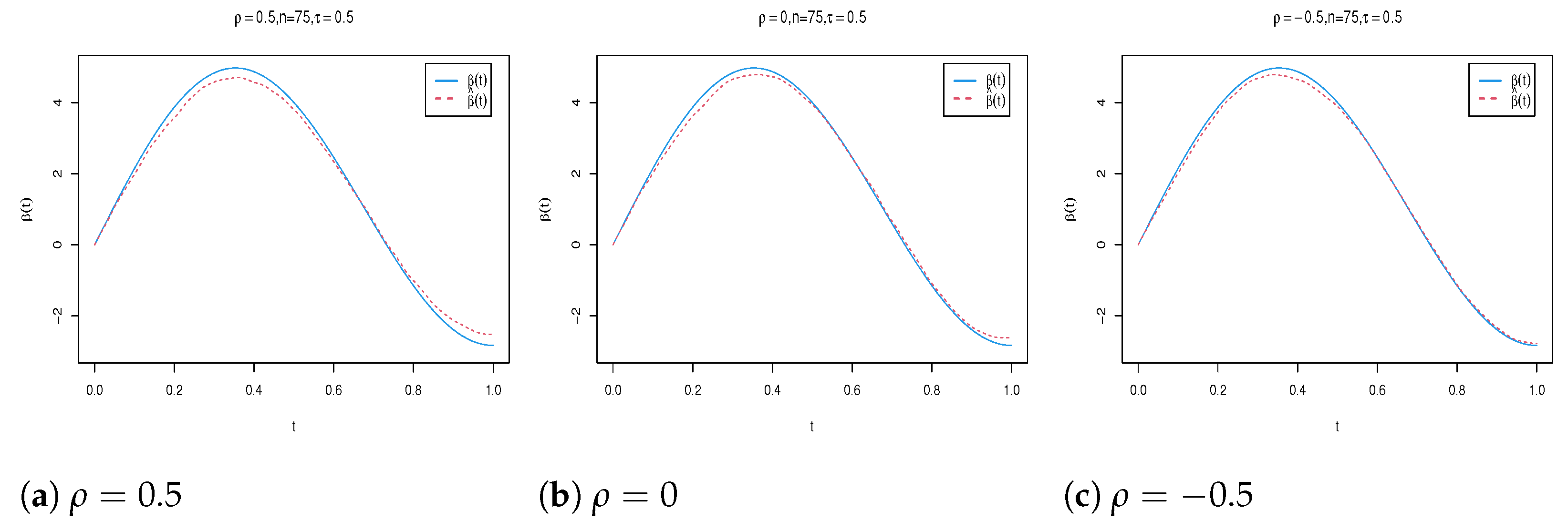
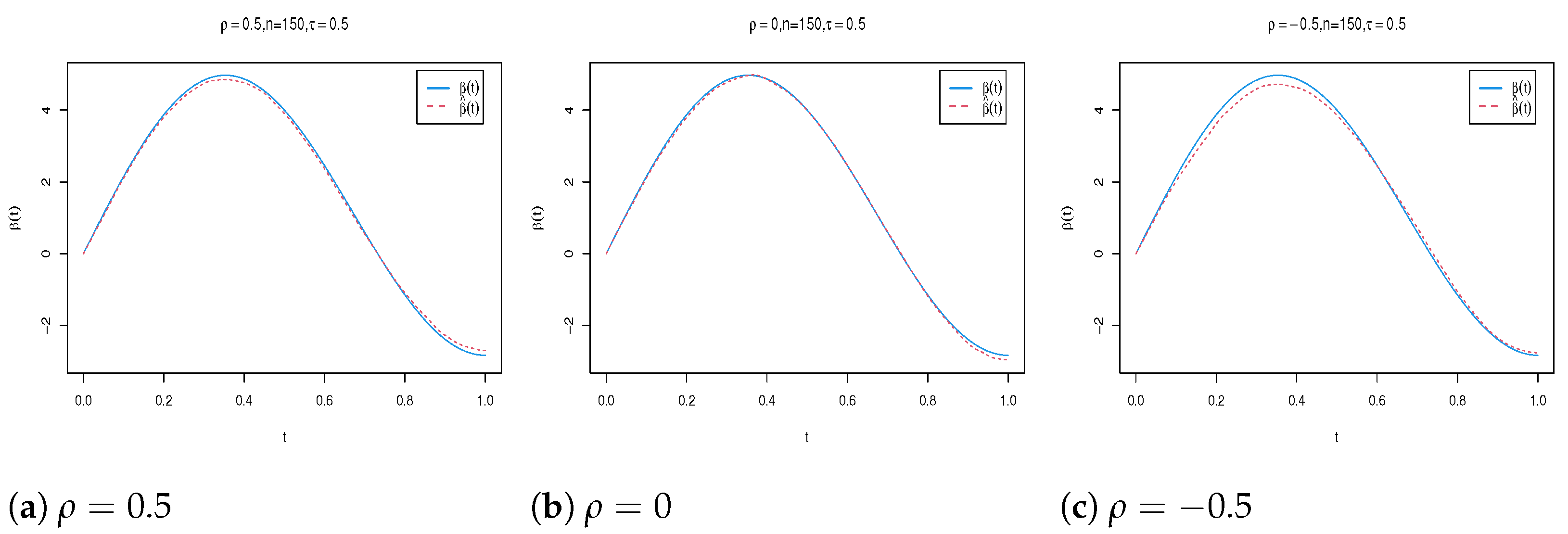
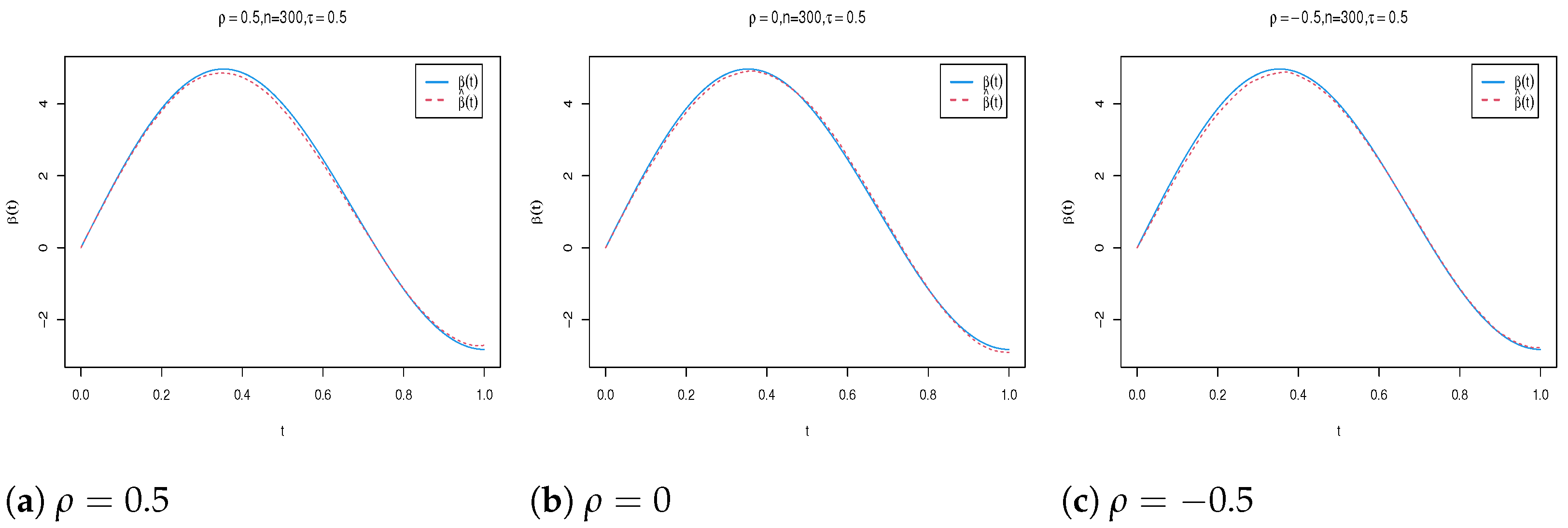
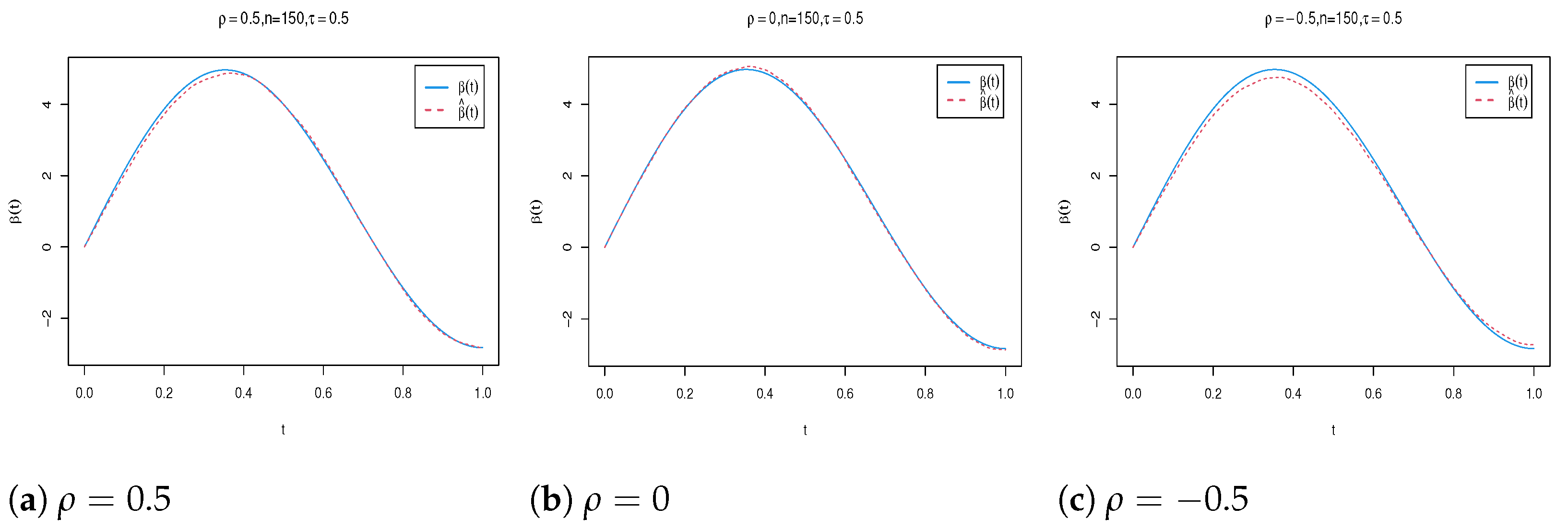
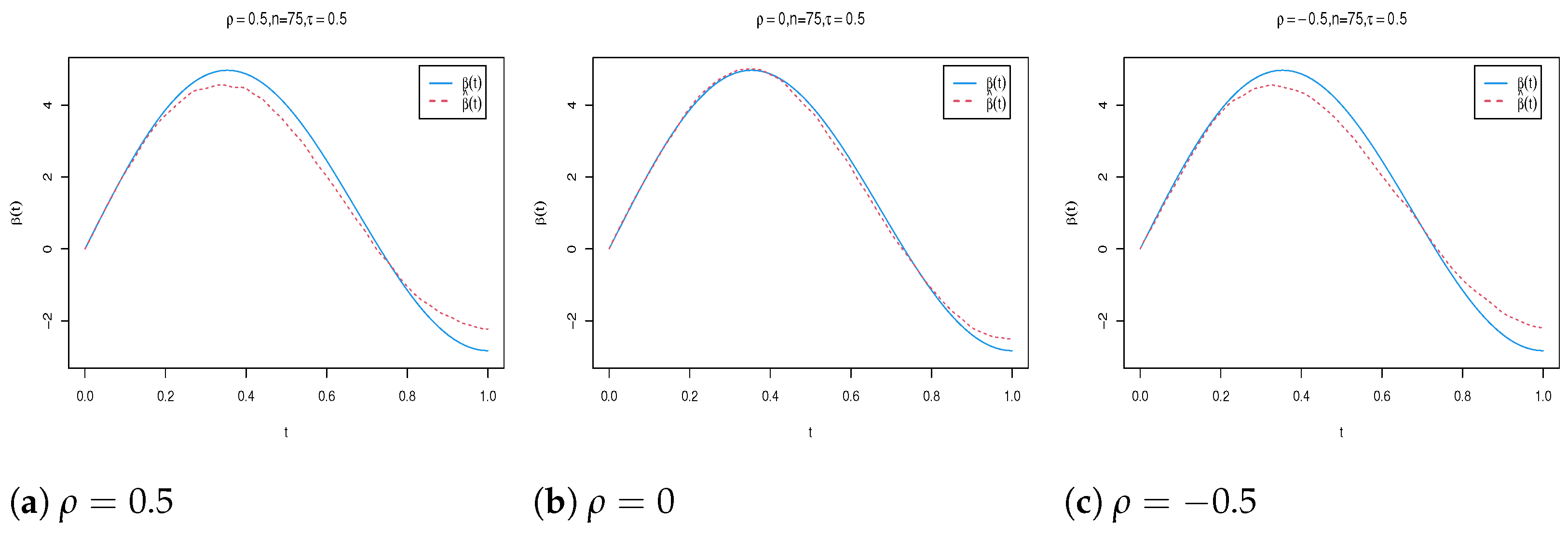
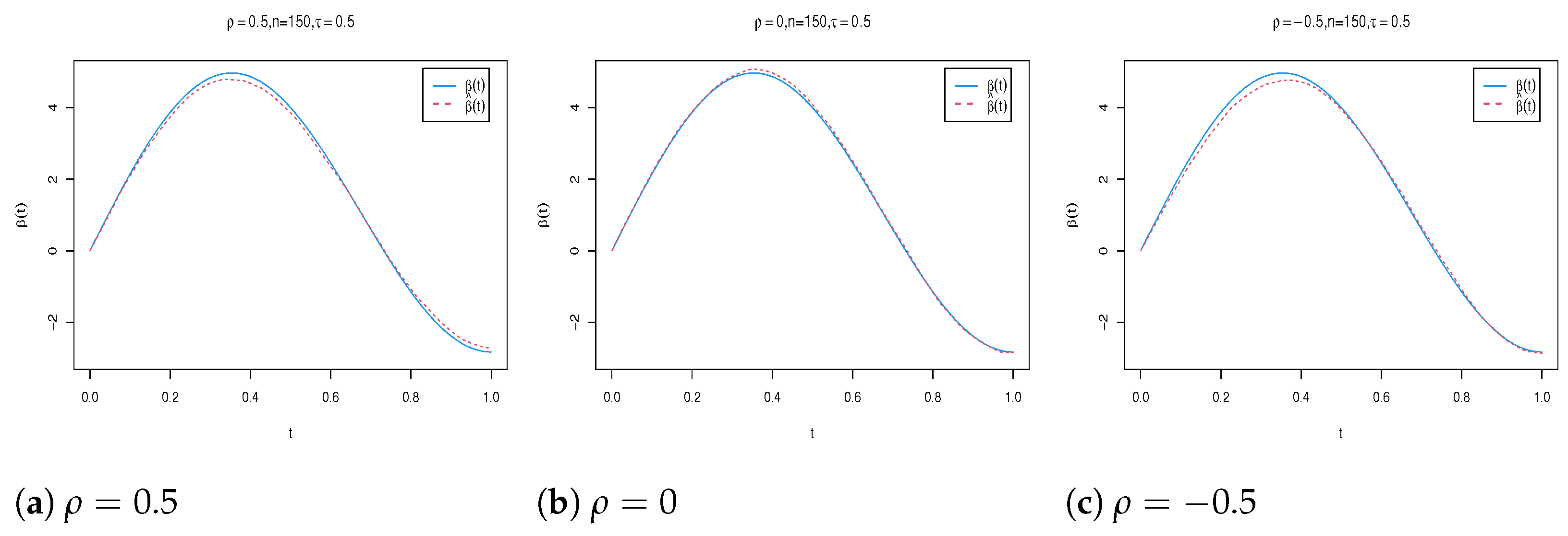
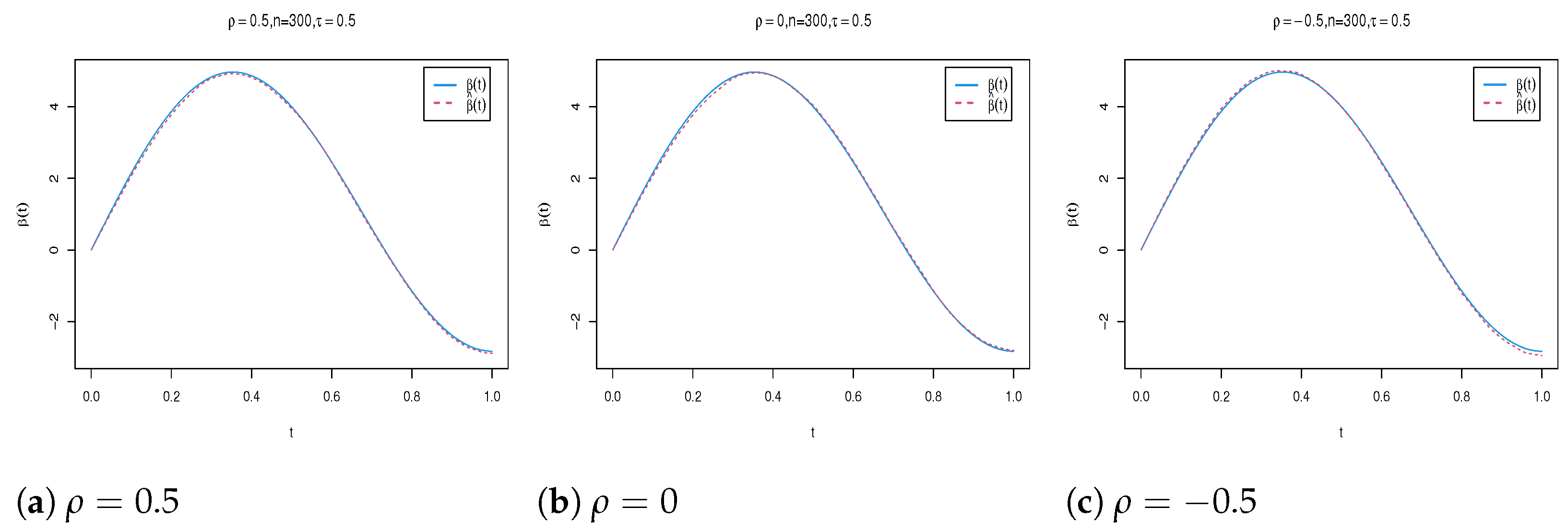
According to the above steps, an efficient MCMC-based sampling algorithm for generating posterior samples from the full conditional distributions of the unknown parameters is constructed. In particular, except the conditional distribution of ρ in (18), the sampling for other parameters are based on familiar distributions and can be easily performed. It is difficult to directly draw the posterior samples from (18) because it is nonstandard. Hence, the Metropolis–Hastings algorithm is used to solve the problem. To begin with, we select normal distribution N ( 0 , σ ρ 2 ) as the proposal distribution, where σ ρ 2 is chosen such that the average acceptance rate is approximately between 0.25 and 0.45. Specifically, the Metropolis–Hastings algorithm is implemented as follows: at the ( l + 1 ) th iteration with the current value ρ ( l ) , a new candidate ρ * is generated from N ( ρ ( l ) , σ ρ 2 ) and is accepted with probability
min 1 , p ( ρ * | Y , Z , X , θ ( l + 1 ) , γ ( l + 1 ) , σ ( l + 1 ) , e ( l + 1 ) ) p ( ρ ( l ) | Y , Z , X , θ ( l + 1 ) , γ ( l + 1 ) , σ ( l + 1 ) , e ( l + 1 ) ) .
Based on the proposed algorithm, we may conclude that the posterior samplers have converged to the joint posterior distribution in (13). Consequently, we can collect M MCMC samples Ψ ( k ) = ( θ ( k ) , γ ( k ) , ρ ( k ) , σ ( k ) ) , for k = 1 , , M , M < J . The Bayesian posterior means of the parameters ( θ ^ , γ ^ , ρ ^ , σ ^ ) are estimated, respectively, as follows
θ ^ = 1 M k = 1 M θ ( k ) , γ ^ = 1 M k = 1 M γ ( k ) , ρ ^ = 1 M k = 1 M ρ ( k ) , σ ^ = 1 M k = 1 M σ ( k ) .

4. Simulation Study

In this section, the performance of the proposed model and Bayesian estimation method will be illustrated through Monte Carlo simulation. All calculations are performed with R 4.3.3. We generate the datasets from the following model:
Y = ρ W Y + Z θ + 0 1 β ( t ) X ( t ) d t + ε ,
where θ = ( 1 , 1 , 2 , 1 ) T and Z follow the multivariate normal distribution N ( 0 , Σ Z ) with the ( i , j ) t h of Σ Z being 0 . 5 | i j | , for i , j = 1 , , 4 . In addition, let the spatial parameter ρ = 0.5 , 0 , 0.5 , which represents different spatial dependencies. Similar to Xie et al. [37], the weight matrix is set to be W = I R H q , H q = ( l q l q T I q ) / ( q 1 ) , where l q is an q-dimensional vector with all elements being 1, ⊗ means Kronecker product, n = R × q . Referring to Shin [5], the functional coefficient β ( t ) = 2 sin ( π t / 2 ) + 3 2 sin ( 3 π t / 2 ) and X ( t ) = j = 1 50 ξ j ϕ j ( t ) are taken, where the ξ j are independently normally distributed with mean 0 and variance λ j = ( ( j 0.5 ) π ) 2 and ϕ j ( t ) = 2 sin ( ( j 0.5 ) π t ) . Furthermore, the noninformative prior information type is considered for hyperparameter values of unknown parameters θ , γ , ρ , σ : μ θ = 0 4 , Σ θ = 10 I 4 , μ γ = 0 m , Σ γ = 10 I m , a σ = b σ = 0.01 , where 0 m is an m-dimensional vector with all elements being 0. Importantly, we determine the truncation level m such that the first m functional principal components scores λ j s can explain at least 90% of the total variability of the functional predictor X ( t ) .
To examine the effect of random error distribution on parameter estimation, we consider the following three distributions for the errors with τ quantile being zero:
  • Case I: ε i N ( μ , 1 ) , with μ such that τ th quantile of ε i is 0;
  • Case II: ε i t ( 3 ) + μ , with μ such that τ th quantile of ε i is 0;
  • Case III: ε i Cauchy ( μ , 1 ) , with μ such that τ th quantile of ε i is 0.
In each type, R is selected as 25, 50, 100 and q is set to 3, and thus, n = 75, 150, 300 at three different quantile levels τ = 0.25 , 0.5 , 0.75 . Based on the above settings and the generated dataset, the preceding proposed hybrid algorithm is used to evaluate the Bayesian estimates of unknown parameters based on 100 replications. Furthermore, we assess the convergence of the proposed hybrid algorithm by calculating the estimated potential scale reduction (EPSR) values [38] for a number of test runs on the base of three parallel chains of observations via three different starting values. In all test runs, the EPSR values are close to 1 and less than 1.2 after 3000 iterations. Therefore, after discarding the initial 3000 iterations in producing the Bayesian estimates for each replication, we can collect M = 2000 observations and present the posterior summary of the parameters in Table 1, Table 2 and Table 3. To evaluate the effect of nonparametric estimators, we also check the square root of average square errors ( R A S E ) defined as:
RASE = 1 N s = 1 N β ^ ( t s ) β ( t s ) 2 1 2 ,
where t s , s = 1 , , N and N = 200 are the grid points at which the function β ^ ( t ) is evaluated. The simulation results are reported in Table 4. Moreover, to visually see the accuracy of estimate of function β ( t ) , we plot the true value of function β ( t ) against its estimate under different cases. Due to space limitations, we only list some nonparametric estimation curve results with different spatial parameters in Figure 1, Figure 2, Figure 3, Figure 4, Figure 5, Figure 6, Figure 7, Figure 8 and Figure 9.
In Table 1, Table 2 and Table 3, “Bias" denotes the absolute difference between the true value and the mean of the Bayesian estimates of the parameters based on 100 replications and “SD" represents standard deviation of the Bayesian estimates. According to Table 1, Table 2, Table 3 and Table 4, we observe that (1) Bayesian estimates are reasonably accurate under all the considered settings because of their relatively small Bias values and SD values. It is also worth noting that Bayesian estimates are quite robust for different error distribution, and the performance under normal error distributions is slightly better than the performance under t and Cauchy error distributions. (2) Based on different spatial parameters and different quantile levels, the results of Bayesian estimation are similar. (3) As the sample size increases, the SD values of all the parameters decrease significantly at each quantile level. (4) For the functional component, the values of RASE decrease with increasing sample size. This indicates that the estimation of functional coefficient β ( t ) is improving. Additionally, Figure 1, Figure 2, Figure 3, Figure 4, Figure 5, Figure 6, Figure 7, Figure 8 and Figure 9 show that the shapes of the estimated nonparametric function closely approximate the corresponding true functional line under all the considered settings, which confirms the results reported in Table 4. In summary, all the above findings demonstrate that the proposed estimation procedure effectively recover the true information in partial functional linear spatial autoregressive model.

5. Conclusions and Discussion

In this paper, we propose a partial functional linear spatial autoregressive model that can effectively study the relationship between a scalar spatial response variable and explanatory variables, including a few scalar variables and a functional random variable. Based on functional principal components analysis, combined with the Gibbs sampler and Metropolis–Hastings algorithm, we develop the Bayesian quantile regression to analyze the model. Extensive simulation studies are conducted to demonstrate the efficiency of the proposed Bayesian approach. As expected, the results show that the developed Bayesian method is satisfactory with high efficiency and fast computation.
In addition, variable selection is an important research direction of functional data analysis, so determining how to consider the robust Bayesian variable selection of the partial functional linear spatial autoregressive model combined with quantile regression is a direction worthy of further study.

Author Contributions

Conceptualization, D.X. and S.K.; methodology, D.X., R.T., J.D. and S.K.; software, S.K. and D.X.; formal analysis, D.X. and S.K.; data curation, S.K. and J.D.; writing—original draft, D.X., S.K., J.D. and R.T.; writing—review and editing, D.X., S.K., J.D. and R.T; supervision, D.X., S.K., J.D. and R.T. All authors have read and agreed to the published version of the manuscript.

Funding

Xu’s work is supported by the Zhejiang Provincial Natural Science Foundation of China under Grant No. LY23A010013, and Dong’s work is supported by the Humanities and Social Sciences Research Project of Ministry of Education under Grant No. 21YJC910002.

Data Availability Statement

The data presented in this study are available on request from the corresponding author.

Conflicts of Interest

The authors declare no conflicts of interest.

References

  1. Yao, F.; Müller, H.; Wang, J. Functional linear regression analysis for longitudinal data. Ann. Stat. 2005, 33, 2873–2903. [Google Scholar] [CrossRef]
  2. Tang, Q.; Kong, L.; Ruppert, D.; Karunamuni, R.J. Partial functional partially linear single-index models. Stat. Sin. 2021, 31, 107–133. [Google Scholar] [CrossRef]
  3. Zhang, X.; Fang, K.; Zhang, Q. Multivariate functional generalized additive models. J. Stat. Comput. Simul. 2022, 92, 875–893. [Google Scholar] [CrossRef]
  4. Rao, A.R.; Reimherr, M. Modern non-linear function-on-function regression. Stat. Comput. 2023, 33, 130. [Google Scholar] [CrossRef]
  5. Shin, H. Partial functional linear regression. J. Stat. Plan. Inference 2009, 139, 3405–3418. [Google Scholar] [CrossRef]
  6. Cui, X.; Lin, H.; Lian, H. Partially functional linear regression in reproducing kernel Hilbert spaces. Comput. Stat. Data Anal. 2020, 150, 106978. [Google Scholar] [CrossRef]
  7. Xiao, P.; Wang, G. Partial functional linear regression with autoregressive errors. Commun. Stat.-Theory Methods 2022, 51, 4515–4536. [Google Scholar] [CrossRef]
  8. Li, T.; Yu, Y.; Marron, J.; Zhu, H. A partially functional linear regression framework for integrating genetic, imaging, and clinical data. Ann. Appl. Stat. 2024, 18, 704–728. [Google Scholar] [CrossRef]
  9. Koenker, R.; Bassett, G., Jr. Regression quantiles. Econom. J. Econom. Soc. 1978, 46, 33–50. [Google Scholar] [CrossRef]
  10. Yang, G.; Liu, X.; Lian, H. Optimal prediction for high-dimensional functional quantile regression in reproducing kernel Hilbert spaces. J. Complex. 2021, 66, 101568. [Google Scholar] [CrossRef]
  11. Zhu, H.; Li, Y.; Liu, B.; Yao, W.; Zhang, R. Extreme quantile estimation for partial functional linear regression models with heavy-tailed distributions. Can. J. Stat. 2022, 50, 267–286. [Google Scholar] [CrossRef] [PubMed]
  12. Xia, L.; Du, J.; Zhang, Z. A Nonparametric Model Checking Test for Functional Linear Composite Quantile Regression Models. J. Syst. Sci. Complex. 2024, 37, 1714–1737. [Google Scholar] [CrossRef]
  13. Ling, N.; Yang, J.; Yu, T.; Ding, H.; Jia, Z. Semi-Functional Partial Linear Quantile Regression Model with Randomly Censored Responses. Commun. Math. Stat. 2024. [Google Scholar] [CrossRef]
  14. Liu, G.; Bai, Y. Functional Quantile Spatial Autoregressive Model and Its Application. J. Syst. Sci. Math. Sci. 2023, 43, 3361–3376. [Google Scholar]
  15. Lee, L.F. Asymptotic distributions of quasi-maximum likelihood estimators for spatial autoregressive models. Econometrica 2004, 72, 1899–1925. [Google Scholar] [CrossRef]
  16. Cheng, S.; Chen, J. Estimation of partially linear single-index spatial autoregressive model. Stat. Pap. 2021, 62, 495–531. [Google Scholar] [CrossRef]
  17. Wang, X.; Shao, J.; Wu, J.; Zhao, Q. Robust variable selection with exponential squared loss for partially linear spatial autoregressive models. Ann. Inst. Stat. Math. 2023, 75, 949–977. [Google Scholar] [CrossRef]
  18. Li, T.; Cheng, Y. Statistical Inference of Partially Linear Spatial Autoregressive Model Under Constraint Conditions. J. Syst. Sci. Complex. 2023, 36, 2624–2660. [Google Scholar] [CrossRef]
  19. Tang, Y.; Du, J.; Zhang, Z. A parametric specification test for linear spatial autoregressive models. Spat. Stat. 2023, 57, 100767. [Google Scholar] [CrossRef]
  20. Xu, D.; Tian, R.; Lu, Y. Bayesian Adaptive Lasso for the Partial Functional Linear Spatial Autoregressive Model. J. Math. 2022, 2022, 1616068. [Google Scholar] [CrossRef]
  21. Liu, G.; Bai, Y. Statistical inference in functional semiparametric spatial autoregressive model. AIMS Math. 2021, 6, 10890–10906. [Google Scholar] [CrossRef]
  22. Hu, Y.; Wang, Y.; Zhang, L.; Xue, L. Statistical inference of varying-coefficient partial functional spatial autoregressive model. Commun. Stat.-Theory Methods 2023, 52, 4960–4980. [Google Scholar] [CrossRef]
  23. Dai, X.; Jin, L. Minimum distance quantile regression for spatial autoregressive panel data models with fixed effects. PLoS ONE 2021, 16, e0261144. [Google Scholar] [CrossRef] [PubMed]
  24. Gu, Y.; You, X.Y. A spatial quantile regression model for driving mechanism of urban heat island by considering the spatial dependence and heterogeneity: An example of Beijing, China. Sustain. Cities Soc. 2022, 79, 103692. [Google Scholar] [CrossRef]
  25. Dai, X.; Li, S.; Jin, L.; Tian, M. Quantile regression for partially linear varying coefficient spatial autoregressive models. Commun. Stat.-Simul. Comput. 2024, 53, 4396–4411. [Google Scholar] [CrossRef]
  26. Han, M. E-Bayesian estimation of the reliability derived from Binomial distribution. Appl. Math. Model. 2011, 35, 2419–2424. [Google Scholar] [CrossRef]
  27. Giordano, M.; Ray, K. Nonparametric Bayesian inference for reversible multidimensional diffusions. Ann. Stat. 2022, 50, 2872–2898. [Google Scholar] [CrossRef]
  28. Chen, Z.; Chen, J. Bayesian analysis of partially linear, single-index, spatial autoregressive models. Comput. Stat. 2022, 37, 327–353. [Google Scholar] [CrossRef]
  29. Yu, C.H.; Prado, R.; Ombao, H.; Rowe, D. Bayesian spatiotemporal modeling on complex-valued fMRI signals via kernel convolutions. Biometrics 2023, 79, 616–628. [Google Scholar] [CrossRef]
  30. Yu, K.; Moyeed, R.A. Bayesian quantile regression. Stat. Probab. Lett. 2001, 54, 437–447. [Google Scholar] [CrossRef]
  31. Yu, Y. Bayesian quantile regression for hierarchical linear models. J. Stat. Comput. Simul. 2015, 85, 3451–3467. [Google Scholar] [CrossRef]
  32. Wang, Z.Q.; Tang, N.S. Bayesian Quantile Regression with Mixed Discrete and Nonignorable Missing Covariates. Bayesian Anal. 2020, 15, 579–604. [Google Scholar] [CrossRef]
  33. Zhang, D.; Wu, L.; Ye, K.; Wang, M. Bayesian quantile semiparametric mixed-effects double regression models. Stat. Theory Relat. Fields 2021, 5, 303–315. [Google Scholar] [CrossRef]
  34. Yu, H.; Yu, L. Flexible Bayesian quantile regression for nonlinear mixed effects models based on the generalized asymmetric Laplace distribution. J. Stat. Comput. Simul. 2023, 93, 2725–2750. [Google Scholar] [CrossRef]
  35. Chu, Y.; Yin, Z.; Yu, K. Bayesian scale mixtures of normals linear regression and Bayesian quantile regression with big data and variable selection. J. Comput. Appl. Math. 2023, 428, 115192. [Google Scholar] [CrossRef]
  36. Yang, K.; Zhao, L.; Hu, Q.; Wang, W. Bayesian quantile regression analysis for bivariate vector autoregressive models with an application to financial time series. Comput. Econ. 2024, 64, 1939–1963. [Google Scholar] [CrossRef]
  37. Xie, T.; Cao, R.; Du, J. Variable selection for spatial autoregressive models with a diverging number of parameters. Stat. Pap. 2020, 61, 1125–1145. [Google Scholar] [CrossRef]
  38. Gelman, A. Inference and monitoring convergence. In Markov Chain Monte Carlo in Practice; CRC Press: Boca Raton, FL, USA, 1996; pp. 131–144. [Google Scholar]
Figure 1. The estimated functional coefficient versus true value of β ( t ) with different ρ s when n = 75 , τ = 0.5 under Case I.
Axioms 14 00467 g001
Figure 2. The estimated functional coefficient versus true value of β ( t ) with different ρ s when n = 150 , τ = 0.5 under Case I.
Axioms 14 00467 g002
Figure 3. The estimated functional coefficient versus true value of β ( t ) with different ρ s when n = 300 , τ = 0.5 under Case I.
Axioms 14 00467 g003
Figure 4. The estimated functional coefficient versus true value of β ( t ) with different ρ s when n = 75 , τ = 0.5 under Case II.
Axioms 14 00467 g004
Figure 5. The estimated functional coefficient versus true value of β ( t ) with different ρ s when n = 150 , τ = 0.5 under Case II.
Axioms 14 00467 g005
Figure 6. The estimated functional coefficient versus true value of β ( t ) with different ρ s when n = 300 , τ = 0.5 under Case II.
Axioms 14 00467 g006
Figure 7. The estimated functional coefficient versus true value of β ( t ) with different ρ s when n = 75 , τ = 0.5 under Case III.
Axioms 14 00467 g007
Figure 8. The estimated functional coefficient versus true value of β ( t ) with different ρ s when n = 150 , τ = 0.5 under Case III.
Axioms 14 00467 g008
Figure 9. The estimated functional coefficient versus true value of β ( t ) with different ρ s when n = 300 , τ = 0.5 under Case III.
Axioms 14 00467 g009
Table 1. Bayesian estimates of unknown parameters under Case I.
ρ nPara. τ = 0.25 τ = 0.5 τ = 0.75
Bias SD Bias SD Bias SD
0.575 θ 1 −0.0310.196 −0.0250.155 −0.0170.192
θ 2 0.0380.216 0.0330.186 0.0060.188
θ 3 −0.0590.241 −0.0560.213 −0.0480.236
θ 4 0.0310.223 0.0100.184 0.0400.194
ρ 0.0530.074 0.0590.086 0.0470.074
150 θ 1 −0.0360.125 −0.0190.128 −0.0360.123
θ 2 0.0490.146 −0.0090.131 0.0420.153
θ 3 −0.0660.171 −0.0610.143 −0.0640.154
θ 4 0.0470.128 0.0390.131 0.0270.125
ρ 0.0570.067 0.0570.067 0.0550.067
300 θ 1 −0.0320.089 −0.0240.089 −0.0400.100
θ 2 0.0330.115 0.0130.092 0.0240.099
θ 3 −0.0610.117 −0.0410.106 −0.0430.108
θ 4 0.0360.094 0.0200.076 0.0180.085
ρ 0.0610.066 0.0580.064 0.0620.066
075 θ 1 −0.0090.182 0.0120.184 −0.0540.186
θ 2 0.0160.241 0.0100.184 0.0570.194
θ 3 −0.0050.218 0.0110.204 −0.0240.205
θ 4 −0.0010.181 0.0000.156 0.0210.198
ρ −0.0210.083 −0.0070.104 −0.0070.104
150 θ 1 0.0280.131 −0.0180.111 0.0280.135
θ 2 0.0180.151 0.0060.122 0.0150.154
θ 3 −0.0310.139 0.0050.119 −0.0050.141
θ 4 0.0090.134 0.0010.124 −0.0120.123
ρ 0.0170.061 −0.0030.065 0.0000.062
300 θ 1 −0.0070.096 −0.0020.079 0.0140.093
θ 2 0.0120.099 0.0030.093 −0.0070.091
θ 3 0.0010.106 0.0070.104 −0.0040.080
θ 4 −0.0140.088 −0.0140.094 0.0030.085
ρ 0.0280.047 −0.0050.046 0.0330.052
−0.575 θ 1 −0.0480.202 −0.0310.179 −0.0500.211
θ 2 0.0340.220 0.0650.184 0.0230.206
θ 3 −0.0610.209 −0.0800.215 −0.0190.216
θ 4 0.0360.209 0.0160.183 −0.0040.181
ρ −0.1100.155 −0.1040.156 −0.1000.148
150 θ 1 −0.0270.131 −0.0200.114 −0.0380.147
θ 2 0.0120.151 0.0200.142 0.0250.145
θ 3 −0.0290.153 −0.0370.148 −0.0500.149
θ 4 0.0180.115 0.0380.140 0.0290.133
ρ −0.0850.119 −0.1070.131 −0.0980.120
300 θ 1 −0.0130.087 −0.0150.089 −0.0210.090
θ 2 0.0210.104 0.0360.110 0.0140.101
θ 3 −0.0280.121 −0.0610.114 −0.0230.108
θ 4 0.0150.106 0.0220.088 0.0160.089
ρ −0.0680.083 −0.1070.119 −0.0660.080
Table 2. Bayesian estimates of unknown parameters under Case II.
ρ nPara. τ = 0.25 τ = 0.5 τ = 0.75
Bias SD Bias SD Bias SD
0.575 θ 1 −0.0360.229 −0.0310.205 −0.0470.242
θ 2 0.0400.233 0.0410.202 0.0510.304
θ 3 −0.0920.296 −0.0510.210 −0.0310.260
θ 4 0.0500.238 0.0290.196 0.0090.250
ρ 0.0680.091 0.0700.089 0.0660.088
150 θ 1 −0.0280.158 −0.0480.134 −0.0380.162
θ 2 0.0460.200 0.0240.143 0.0280.177
θ 3 −0.0950.228 −0.0530.154 −0.0590.176
θ 4 0.0390.169 0.0290.147 0.0550.166
ρ 0.0790.086 0.0700.085 0.0760.084
300 θ 1 −0.0280.118 −0.0240.088 −0.0260.100
θ 2 0.0230.115 0.0180.097 0.0140.120
θ 3 −0.0560.134 −0.0550.111 −0.0700.143
θ 4 0.0210.112 0.0310.097 0.0510.128
ρ 0.0800.084 0.0790.084 0.0760.081
075 θ 1 0.0100.247 −0.0360.203 −0.0410.204
θ 2 −0.0180.302 0.0340.270 0.0460.252
θ 3 0.0010.245 −0.0220.211 0.0260.293
θ 4 0.0260.211 −0.0040.242 −0.0260.253
ρ −0.0060.103 −0.0160.115 −0.0120.108
150 θ 1 −0.0010.156 −0.0040.145 −0.0020.161
θ 2 −0.0070.194 0.0000.151 −0.0150.191
θ 3 0.0060.166 −0.0080.149 0.0070.175
θ 4 −0.0080.169 −0.0030.134 −0.0080.148
ρ 0.0000.062 0.0010.063 0.0090.063
300 θ 1 −0.0040.105 −0.0200.095 0.0010.106
θ 2 −0.0120.120 0.0110.107 −0.0130.120
θ 3 −0.0130.121 0.0100.106 −0.0060.141
θ 4 0.0080.097 0.0000.088 0.0050.114
ρ 0.0260.056 −0.0060.053 0.0220.059
−0.575 θ 1 −0.0410.240 −0.0390.175 −0.0200.247
θ 2 0.0580.272 0.0230.204 0.0750.260
θ 3 −0.1030.324 −0.0500.254 −0.1270.313
θ 4 0.0380.252 0.0440.202 0.0750.258
ρ −0.1600.205 −0.1500.185 −0.1440.201
150 θ 1 −0.0310.147 −0.0420.146 −0.0290.186
θ 2 0.0430.177 0.0430.179 0.0570.193
θ 3 −0.0550.194 −0.0810.177 −0.0930.214
θ 4 0.0260.181 0.0390.148 0.0460.175
ρ −0.1300.162 −0.1490.174 −0.1310.156
300 θ 1 −0.0450.124 −0.0370.105 −0.0240.128
θ 2 0.0440.151 0.0280.109 0.0470.121
θ 3 −0.0610.153 −0.0590.127 −0.0590.131
θ 4 0.0260.112 0.0400.103 0.0140.109
ρ −0.1340.148 −0.1590.171 −0.1090.127
Table 3. Bayesian estimates of unknown parameters under Case III.
ρ nPara. τ = 0.25 τ = 0.5 τ = 0.75
Bias SD Bias SD Bias SD
0.575 θ 1 −0.0180.364 −0.0780.340 −0.0540.321
θ 2 −0.0290.448 0.0260.339 0.0510.487
θ 3 −0.0540.466 −0.0240.356 −0.0720.457
θ 4 0.0480.377 0.0220.300 0.0650.474
ρ 0.0870.098 0.0790.094 0.0840.101
150 θ 1 −0.0180.237 −0.0570.186 −0.0380.301
θ 2 −0.0050.268 0.0300.203 −0.0030.298
θ 3 −0.0320.319 −0.0410.197 −0.0350.288
θ 4 0.0260.255 0.0130.167 0.0010.210
ρ 0.0620.077 0.0660.076 0.0870.096
300 θ 1 −0.0410.184 −0.0060.121 −0.0400.181
θ 2 0.0090.189 0.0060.111 0.0140.180
θ 3 −0.0490.184 −0.0320.124 −0.0260.197
θ 4 0.0390.180 0.0290.107 0.0140.168
ρ 0.0560.065 0.0350.048 0.0520.066
075 θ 1 −0.0200.382 0.0300.295 0.0100.326
θ 2 −0.0410.457 −0.0470.286 0.0370.386
θ 3 0.0070.541 0.0660.331 −0.0080.395
θ 4 −0.0370.409 −0.0340.253 0.0320.340
ρ −0.0280.190 −0.0050.140 0.0230.120
150 θ 1 0.0250.245 −0.0260.160 0.0260.294
θ 2 −0.0250.304 0.0260.202 −0.0200.340
θ 3 −0.0430.296 −0.0310.190 −0.0390.332
θ 4 0.0220.242 0.0060.156 0.0120.248
ρ −0.0020.101 −0.0060.098 0.0300.109
300 θ 1 −0.0260.212 −0.0080.120 −0.0120.174
θ 2 −0.0060.209 −0.0150.135 0.0290.201
θ 3 0.0410.193 0.0290.137 −0.0100.204
θ 4 0.0080.172 −0.0190.112 −0.0230.188
ρ 0.0070.096 0.0000.066 0.0110.060
−0.575 θ 1 −0.0340.515 −0.0480.304 −0.0780.472
θ 2 0.0020.548 0.0450.336 0.1300.479
θ 3 −0.0510.549 −0.0680.359 −0.0790.465
θ 4 0.0800.471 0.0030.312 −0.0270.397
ρ −0.1620.212 −0.1390.191 −0.1390.180
150 θ 1 −0.0010.286 −0.0240.168 −0.0440.276
θ 2 0.0270.358 0.0560.188 0.0750.333
θ 3 −0.0520.301 −0.0700.217 −0.0220.352
θ 4 0.0000.264 0.0200.181 0.0040.313
ρ −0.1290.166 −0.1080.143 −0.1370.178
300 θ 1 −0.0150.206 −0.0050.111 −0.0130.192
θ 2 0.0390.209 0.0160.125 −0.0030.231
θ 3 −0.0750.203 −0.0440.136 −0.0600.228
θ 4 0.0770.179 0.0270.129 0.0410.196
ρ −0.1210.143 −0.0830.098 −0.1250.146
Table 4. The values of RASE for the nonparametric components under different cases.
ρ n τ Case ICase IICase III
0.575 0.25 1.0551.2341.751
0.5 0.9441.0361.490
0.75 0.9341.1011.686
150 0.25 0.6770.8771.262
0.5 0.6380.6930.849
0.75 0.6880.7701.189
300 0.25 0.4380.5470.785
0.5 0.4190.5080.561
0.75 0.4870.5140.790
075 0.25 1.0431.2631.897
0.5 0.8841.0181.310
0.75 1.0211.0801.944
150 0.25 0.7020.7711.156
0.5 0.6190.6571.007
0.75 0.6210.7961.233
300 0.25 0.5050.5430.806
0.5 0.4550.4840.568
0.75 0.4810.5690.815
−0.575 0.25 1.0991.1641.816
0.5 0.8720.9971.397
0.75 1.0661.1561.817
150 0.25 0.6850.8501.275
0.5 0.6390.7090.842
0.75 0.7480.7651.359
300 0.25 0.4510.5880.848
0.5 0.4770.5140.542
0.75 0.4840.5330.933
Disclaimer/Publisher’s Note: The statements, opinions and data contained in all publications are solely those of the individual author(s) and contributor(s) and not of MDPI and/or the editor(s). MDPI and/or the editor(s) disclaim responsibility for any injury to people or property resulting from any ideas, methods, instructions or products referred to in the content.

