From Different Systems to a Single Common Model: A Review of Dynamical Systems Leading to Lorenz Equations

Abstract

This paper presents an analytical exploration of how diverse dynamical systems, arising from different scientific domains, can be reformulated (under specific approximations and assumptions) into a common set of equations formally equivalent to the Lorenz system originally derived to model atmospheric convection. Unlike previous studies that focus on analyzing or applying the Lorenz equations, our objective is to show how these equations emerge from distinct models, emphasizing the underlying structural and dynamical similarities. The mathematical steps involved in these reformulations are included. The systems examined include Lorenz’s original atmospheric convection model, the chaotic water wheel, the Maxwell–Bloch equations for lasers, mechanical gyrostat, solar dynamo model, mesoscale reaction dynamics, an interest rate economic model, and a socioeconomic control system. This work includes a discussion of the unifying features that lead to similar qualitative behaviors across seemingly unrelated systems. By highlighting the Lorenz system as a paradigmatic limit of a broad class of nonlinear models, we underscore its relevance as a unifying framework in the study of complex dynamics.

1. Introduction

In 1963, meteorologist Edward Lorenz published an article entitled “Deterministic Nonperiodic Flow” [1], introducing the now well-known Lorenz equations. This system of three differential equations was originally formulated as a simplified representation of the Rayleigh–Bénard problem [2], aiming to model convection processes in the atmosphere. Since then, the Lorenz system has become one of the most extensively studied low-dimensional chaotic systems worldwide [3,4,5]. In particular, it exhibits periodic and chaotic behavior with highly distinctive characteristics, paving the way for the development of chaos theory in dynamical systems.

Today, the Lorenz system serves as a paradigmatic model for analyzing nonlinear systems across various domains, including chaos theory, the geometric properties of dynamical systems, nonlinear time series analysis, synchronization, and the stabilization of coupled systems [6,7,8].

One research direction of the Lorenz equations focuses on their application in describing various phenomena using this model. Over time, the Lorenz system has been extended and adapted, leading to different formulations that can be categorized based on the type of partial differential equations involved [9]. Among these applications, notable examples include the butterfly effect, where the Lorenz equations have been used to provide an explanation for the underlying dynamics [10].

However, in an insightful study, Sprott [11] presented several systems exhibiting inherently complex behavior. In that work, the author raised the question of whether such systems share common dynamical properties.

A key aspect of these findings is their broad applicability across diverse research fields (including mechanics, electronics, biology, and economics), where various phenomena can be described using the Lorenz equations or equivalent models. Although the parameters and dynamics of these models are constrained by specific mathematical formulations, their underlying principles remain widely relevant.

An intriguing question arises regarding the fundamental properties that enable these systems to exhibit similar dynamic behavior. This paper explores some of these systems as a means of understanding and explaining such phenomena. Additionally, an effort has been made to present the discussion in an accessible manner for students with limited prior knowledge of the subject.

Both the Lorenz equations and their solutions have been extensively studied in numerous works [12,13,14,15]. Unlike these studies, the primary objective of this article is to demonstrate how the Lorenz equations can be derived from certain dynamical systems, highlighting the approximations and assumptions involved in each case. Additionally, we provide insights into the remarkably similar dynamic behavior observed across seemingly unrelated systems.

In other words, this work focuses on reformulating equations from various dynamical systems to show that, under specific conditions, they can coincide with the Lorenz equations. However, we do not adopt the reverse approach of reviewing direct applications of the Lorenz equations to describe specific phenomena.

This paper is structured as follows: Section 2 examines Lorenz’s original problem of atmospheric convection cells. In Section 3, the classical system of the chaotic water wheel is introduced. Section 4 explores a system governed by the Maxwell–Bloch equations for lasers. In Section 5, a mechanical system represented by the gyrostat is analyzed, followed by a solar dynamo model in Section 6. Section 7 discusses mesoscale dynamics in chemical reactions. An economic model for interest rates is presented in Section 8, while Section 9 examines a socioeconomic control system. Finally, the analysis and conclusions are provided in Section 10.

2. Rayleigh–Bénard Convection

In 1963, meteorologist Edward Lorenz developed a system of three coupled ordinary differential equations to describe fluid motion under the influence of a thermal gradient [16]. While computing numerical solutions, he observed an unexpected phenomenon: the system exhibited extreme sensitivity to initial conditions. Even the slightest variations in initial values led to drastically different solutions, rendering the system inherently unpredictable.

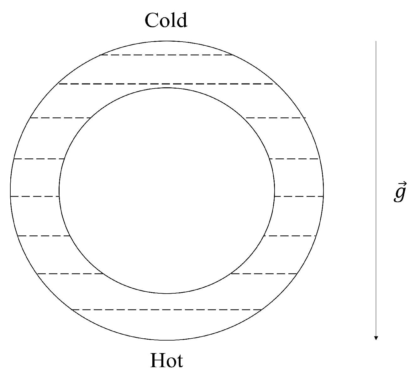
Convection plays a crucial role in atmospheric dynamics. Inspired by fluid dynamics, Lorenz sought to derive a set of equations describing the behavior of a heated gas or liquid within a confined cell (see Figure 1). This phenomenon, which can be experimentally reproduced, is widely known as Rayleigh–Bénard convection.

The Rayleigh–Bénard convection phenomenon can be modeled based on previous studies [17,18,19,20]. As a simplification, we consider a two-dimensional case, where the plates extend infinitely in the horizontal direction, x, while the temperature gradient is applied in the vertical direction, y. In Figure 1, the loop is defined in the $x-y$ plane, with the cylinders oriented parallel to the z axis. The state of the system is characterized by the velocity v, temperature T, and pressure p.

The Lorenz equations describing the convection phenomenon are derived following the approach in [19], which, in turn, is based on the original derivation in [21]. The governing hydrodynamic equations for convection, based on the Navier–Stokes formulation, are given by Equation (1):

$$\begin{array}{ccc}\hfill {\displaystyle \frac{\partial \overrightarrow{v}}{\partial t}}+\overrightarrow{v}·\nabla \overrightarrow{v}& =& -{\displaystyle \frac{1}{\rho }}\nabla p-\alpha \overrightarrow{g}\Delta T+u{\nabla }^2\overrightarrow{v}\hfill \\ \hfill {\displaystyle \frac{\partial T}{\partial t}}+\overrightarrow{v}·\nabla T& =& \kappa {\nabla }^{2}T\hfill \\ \hfill \nabla ·\overrightarrow{v}& =& 0.\hfill \end{array}$$

(1)

The first equation represents momentum conservation (the Navier–Stokes equation), the second describes temperature evolution, and the third corresponds to mass conservation. Here, $\rho$ denotes fluid density, $\kappa$ represents the fluid-specific diffusivity, $\alpha$ is the coefficient of expansion of the fluid, and u indicates the kinematic viscosity. The temperature difference, $\Delta T=T_B-T_A$, acts as a control parameter that can be adjusted. Additionally, the symbol “·” denotes the scalar product, while $\nabla =\left({\displaystyle \frac{\partial }{\partial x}},{\displaystyle \frac{\partial }{\partial y}},{\displaystyle \frac{\partial }{\partial z}}\right)$ represents the nabla differential operator. Moreover, ${\nabla }^2=\left({\displaystyle \frac{{\partial }^2}{\partial x^2}},{\displaystyle \frac{{\partial }^2}{\partial y^2}},{\displaystyle \frac{{\partial }^2}{\partial z^2}}\right)$ corresponds to the Laplacian operator.

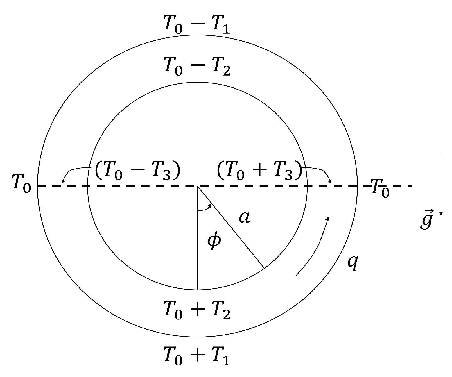
It would now be considered a vertical torus filled with fluid, which is heated at the bottom and cooled at the top in a manner that preserves symmetry between the left and right sides. The torus can be observed in Figure 2. Since the fluid becomes lighter at the bottom and denser at the top, it is expected to have a convective motion around the torus. For the subsequent analysis, various quantities relevant to this setup are presented in Figure 3, where the position along the loop is indicated by the angle $\varphi$.

The external temperature $T_E$ varies linearly with height and is defined by Equation (2):

$$T_E=T_0+T_{1}cos\left(\varphi \right)$$

(2)

Inside the convection cylinder, in a cross-section, the average speed $q=q(\varphi ,t)$ and temperature $T=T(\varphi ,t)$ depend only on $\varphi$ and t. For an incompressible fluid, the Equation (3) must be satisfied:

$${\displaystyle \frac{\partial q}{\partial \varphi }}=0.$$

(3)

This implies that motion within the system is equivalent to that of a rotating solid. Additionally, if Equation (3) is satisfied (the continuity equation), it indicates that q is only function of t. In other words, $q(\varphi ,t)\to q\left(t\right)$.

In addition, the temperature variation round the loop follows the expression given in Equation (4):

$$T-T_0=T_{2}cos\left(\varphi \right)+T_{3}sin\left(\varphi \right)$$

(4)

The Navier–Stokes equation in this case is expressed as Equation (5) [19].

$${\displaystyle \frac{\partial q}{\partial t}}=-{\displaystyle \frac{1}{\rho a}}{\displaystyle \frac{\partial p}{\partial \varphi }}+g\alpha (T-T_0)sin\left(\varphi \right)-\Gamma q$$

(5)

where $\Gamma$ represents a generalized friction coefficient related to viscosity and is proportional to velocity.

By substituting $T-T_0$ from Equation (4) into the Equation (5) and integrating with respect to $\varphi$ over a full cycle (i.e., from 0 to $2\pi$), the resultant integral is displayed in Equation (6).

$$2\pi {\displaystyle \frac{dq}{dt}}=g\alpha {\int }_0^{2\pi }\left(T_{2}cos\left(\varphi \right)sin\left(\varphi \right)+T_3{sin}^2\left(\varphi \right)\right)d\varphi -2\pi \Gamma q$$

(6)

The Equation (6) can be simplified to Equation (7), demonstrating that horizontal motion is driven solely by temperature differences.

$${\displaystyle \frac{dq}{dt}}=-\Gamma q+{\displaystyle \frac{g\alpha T_3}{2}}$$

(7)

For the temperature equation, we assume $T=T(\varphi ,t)$. By averaging over the cross-section of the ring, the temperature is determined by Equation (8) [19].

$${\displaystyle \frac{\partial T}{\partial t}}+{\displaystyle \frac{q}{a}}{\displaystyle \frac{\partial T}{\partial \varphi }}=K(T_E-T)$$

(8)

where K represents the heat transfer coefficient, and $T_E$ is the external temperature, which varies linearly with height; it is also assumed to produce negligible conduction along the ring.

Substituting $T_E$ from Equation (2) and T from Equation (4) into Equation (8) yields Equation (9):

$${\displaystyle \frac{d{T}_2}{dt}}cos\varphi +{\displaystyle \frac{q{T}_3}{a}}cos\varphi +{\displaystyle \frac{d{T}_3}{dt}}sin\varphi -{\displaystyle \frac{q{T}_2}{a}}sin\varphi =K(T_1-T_2)cos\varphi -K{T}_{3}sin\varphi .$$

(9)

By examining the sine and cosine terms, Equation (9) holds for all values of $\varphi$ if Equations (10) and (11) are satisfied:

$${\displaystyle \frac{d{T}_3}{dt}}-{\displaystyle \frac{q{T}_2}{a}}=-K{T}_3,$$

(10)

$${\displaystyle \frac{d{T}_2}{dt}}+{\displaystyle \frac{q{T}_3}{a}}=K(T_1-T_2).$$

(11)

We introduce the variable $T_4=T_1-T_2$, which represents the deviation of the fluid temperature from the external temperature at the top or bottom of the loop. Substituting $T_2=T_1-T_4$ into Equations (10) and (11) leads to the reformulated system given by Equations (12) and (13):

$${\displaystyle \frac{d{T}_3}{dt}}=-K{T}_3+{\displaystyle \frac{q{T}_1}{a}}-{\displaystyle \frac{q{T}_4}{a}},$$

(12)

$${\displaystyle \frac{d{T}_4}{dt}}=-K{T}_4+{\displaystyle \frac{q{T}_3}{a}}.$$

(13)

Next, the following change of variables of Equation (14) and the introduction of a dimensionless time parameter, $t^{\prime }=tK$, are applied to Equations (7), (12), and (13):

$$X={\displaystyle \frac{q}{aK}},Y={\displaystyle \frac{g\alpha T_3}{2a\Gamma K}},Z={\displaystyle \frac{g\alpha T_4}{2a\Gamma K}},\sigma ={\displaystyle \frac{\Gamma }{K}},r={\displaystyle \frac{g\alpha T_1}{2a\Gamma K}}$$

(14)

As a result, the system is transformed into Equations (15), (16), and (17), respectively.

$${\displaystyle \frac{dX}{dt}}=-\sigma X+\sigma Y$$

(15)

$${\displaystyle \frac{dY}{dt}}=-Y+rX-XZ$$

(16)

$${\displaystyle \frac{dZ}{dt}}=-Z+XY.$$

(17)

where

• X: The amplitude of the convective motion.
• Y: The temperature difference between upstream and downstream currents.
• Z: The deviation from the conductive equilibrium of the system.

Here, $\sigma$ is the Prandtl number, a dimensionless quantity characterizing the fluid’s viscosity, and r is the Reynolds number, which describes fluid flow behavior.

These equations, known as the Lorenz equations, provide first-order equations resembling to the hydrodynamic equations governing convection in a Rayleigh–Bénard system, as described in Equation (1).

3. Chaotic Water Wheel

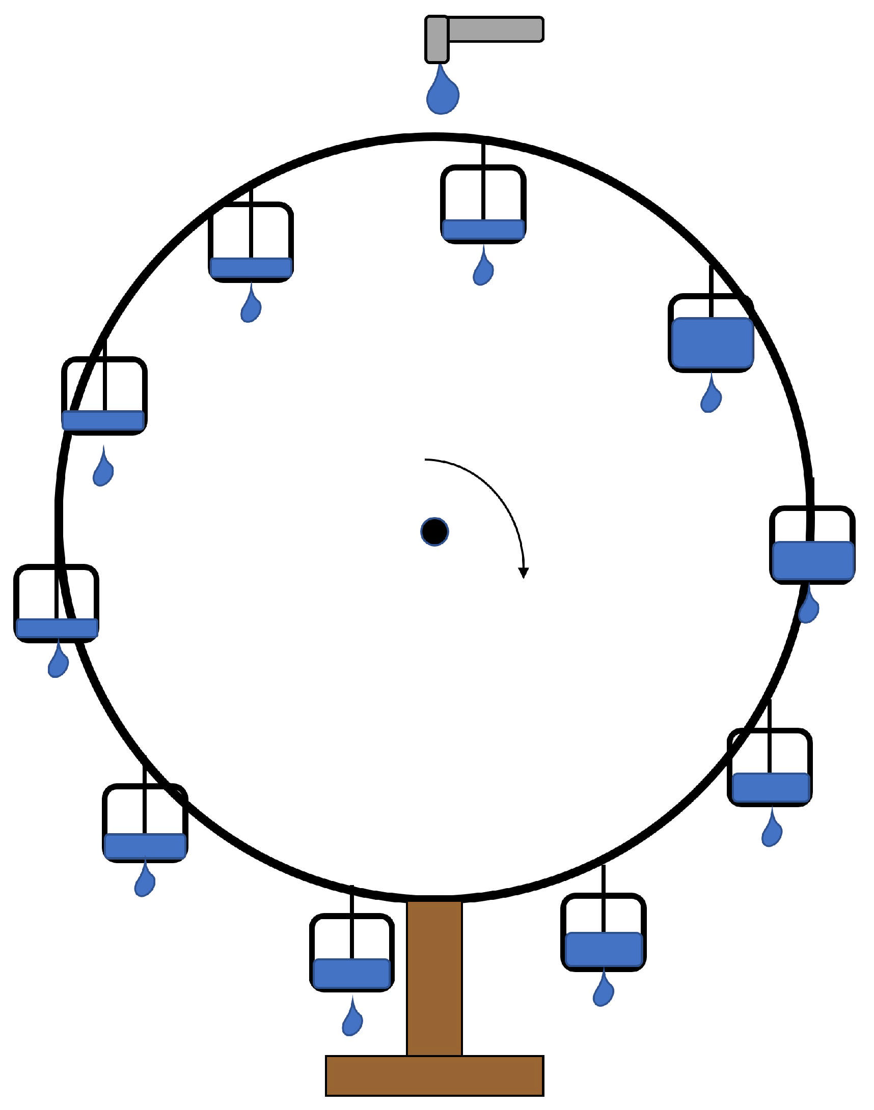
The chaotic water wheel is a mechanical system whose dynamics are governed by a set of equations equivalent to the Lorenz model. Originally conceived by W. Malkus and L. Howard in the 1970s [16,22,23,24], this system consists of a rotating wheel with small, fixed containers attached along its perimeter. These containers are perforated at the bottom, allowing water to drain as the wheel moves. The wheel rotates freely around an axis at a variable angle relative to the horizontal plane.

Water is continuously supplied from above, filling the containers as they move along the wheel’s perimeter. If the inflow rate is low, the containers do not accumulate enough water to overcome frictional forces, and the wheel remains at rest. However, if the inflow rate increases sufficiently to fill the containers, the accumulated weight initiates rotation. Due to the system’s symmetry, the wheel may rotate in either direction, depending on its initial conditions (see Figure 4).

As the inflow continues to increase, the system exhibits a transition from steady rotation to chaotic behavior. Initially, the wheel rotates in a single direction for multiple turns. However, as some containers become completely filled, the wheel may lose the necessary inertia to carry them to the top. Consequently, it slows down, and in some cases, it may even reverse direction. This leads to erratic and unpredictable oscillations in the wheel’s rotation.

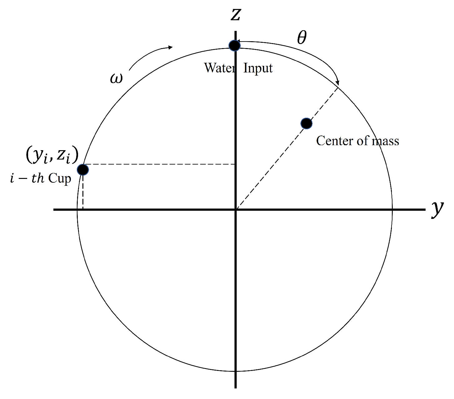
To analyze the system’s dynamics [25,26,27], the following variables are defined:

• $\theta$: The angular position of the wheel, measured from the initial position, where $\theta =0$ corresponds to the top of the wheel.
• $\omega \left(t\right)$: The angular velocity of the wheel.
• $m(\theta ,t)$: The mass distribution of water along the wheel’s perimeter, representing the mass between angles ${\theta }_1$ and ${\theta }_2$.

$$M\left(t\right)={\int }_{{\theta }_1}^{{\theta }_2}m(\theta ,t)d\theta .$$

Additionally, the following variables are introduced:

• $Q\left(\theta \right)$: The inflow rate, representing the amount of water entering the system at position $\theta$.
• r: The wheel’s radius.
• K: The drainage rate of the containers.
• v: The rotational viscosity coefficient.
• l: The moment of inertia of the wheel (see Figure 5).

Using the mass continuity principle, Equation (18) is obtained, whose explicit derivation can be found in [25]. This equation results in a partial differential equation that describes the evolution of $m(\theta ,t)$.

$${\displaystyle \frac{\partial m}{\partial t}}=Q-Km-\omega {\displaystyle \frac{\partial m}{\partial \theta .}}$$

(18)

The remaining unknown variable in the system is $\omega \left(t\right)$, which is the angular velocity of the wheel. The wheel’s rotation is governed by Newton’s second law, $F=ma$, which, in this case, is expressed in terms of applied torques and the rate of change of angular momentum. Since the moment of inertia of the wheel, l, depends on time t due to the changing distribution of water, the equation of motion can be written as Equation (19).

$$l\dot{\omega }=\mathrm{damping}\mathrm{torque}+\mathrm{gravitational}\mathrm{torque}.$$

(19)

where the damping torque is defined in Equation (20), and the gravitational torque is discussed below:

$$\mathrm{damping}\mathrm{torque}=-v\omega .$$

(20)

The system experiences two sources of damping: One arises from the natural resistance at the wheel’s axle, while the other is induced by the inflow of water, which influences the wheel’s spin. The effective gravitational constant is given by $g=g_{n}sin\left(\alpha \right)$, where (g_n = 9.81 m/s²) is the standard gravitational acceleration, and $\alpha$ represents the angle between the wheel’s axis and the horizontal plane.

To determine the gravitational contribution, we integrate over all mass elements distributed along the wheel’s perimeter, yielding Equation (21):

$$\mathrm{gravitational}\mathrm{torque}=gr{\int }_0^{2\pi }m(\theta ,t)sin\left(\theta \right)d\theta$$

(21)

By incorporating both the damping and gravitational torques from Equations (20) and (21), we obtain the equation of motion as Equation (22):

$$l\dot{\omega }=-v\omega +gr{\int }_0^{2\pi }m(\theta ,t)sin\left(\theta \right)d\theta ,$$

(22)

which represents a balance of torques acting on the system.

Since $m(\theta ,t)$ is periodic in $\theta$, it can be expressed as a Fourier series, as shown in Equation (23):

$$m(\theta ,t)=\sum _{n=0}^{\infty }\left[a_n\left(t\right)sin\left(n\theta \right)+b_n\left(t\right)cos\left(n\theta \right)\right].$$

(23)

Substituting Equation (23) into Equation (22), we obtain Equation (24):

$$l\dot{\omega }=-v\omega +gr{\int }_0^{2\pi }\sum _{n=0}^{\infty }\left[a_n\left(t\right)sin\left(n\theta \right)+b_n\left(t\right)cos\left(n\theta \right)\right]sin\left(\theta \right)d\theta$$

(24)

By orthogonality, Equation (25) holds

$$\sum _{n=0}^{\infty }\left[a_n\left(t\right)sin\left(n\theta \right)+b_n\left(t\right)cos\left(n\theta \right)\right]sin\left(\theta \right)=a_1{sin}^2\left(\theta \right)$$

(25)

Substituting Equation (25) into Equation (24) and integrating, we arrive at Equation (26):

$$l\dot{\omega }=-v\omega +gr{\int }_0^{2\pi }{a}_1{sin}^2\left(\theta \right)d\theta =-v\omega +gr{a}_1\pi$$

(26)

However, the inflow Q can also be expressed as a Fourier series in Equation (27), where the absence of sine terms is due to the symmetric addition of water at the top of the wheel:

$$Q\left(\theta \right)=\sum _{n=0}^{\infty }{q}_{n}cosn\theta .$$

(27)

Substituting both series for m from Equation (23) and for Q from Equation (27) into Equation (18), we obtain the resulting Equation (28):

$$\begin{array}{cc}\hfill {\displaystyle \frac{\partial }{\partial t}}\left[\sum _{n=0}^{\infty }\left(a_n\left(t\right)sinn\theta +b_n\left(t\right)cosn\theta \right)\right]& =-\omega {\displaystyle \frac{\partial }{\partial \theta }}\left[\sum _{n=0}^{\infty }\left(a_n\left(t\right)sinn\theta +b_n\left(t\right)cosn\theta \right)\right]\hfill \\ \hfill & +\sum _{n=0}^{\infty }{q}_{n}cosn\theta \hfill \\ \hfill & -K\left[\sum _{n=0}^{\infty }\left(a_n\left(t\right)sinn\theta +b_n\left(t\right)cosn\theta \right)\right].\hfill \end{array}$$

(28)

By the orthogonality of the basis functions, the coefficients of each harmonic in Equation (28) can be equated separately. In particular, the coefficient of $sin\left(n\theta \right)$ for $n=0,1,\dots$ on the left-hand side is ${\dot{a}}_n$, while on the right-hand side, it is given by $n\omega b_n-K{a}_n$, leading to Equation (29):

$${\dot{a}}_n=n\omega b_n-K{a}_n.$$

(29)

Similarly, equating the coefficients of $cos\left(n\theta \right)$ results in Equation (30):

$${\dot{b}}_n=-n\omega a_n-K{b}_n+q_n.$$

(30)

Notably, only $a_1$ appears in the differential equation for $\dot{\omega }$. However, the equations governing $\dot{a_1}$ and $\dot{b_1}$ can be computed using Equations (29) and (30) for $n=1$. In conclusion, $\dot{a_1}$, $\dot{b_1}$, and Equation (24) form a closed system. These three variables are independent of all other coefficients $\dot{a_n}$ and $\dot{b_n}$ for $n\ne 1$. Consequently, the system’s evolution is described by the following set of equations described in Equation (31).

$$\begin{array}{ccc}\hfill \dot{\omega }& =& -{\displaystyle \frac{v}{l}}\omega +{\displaystyle \frac{gr\pi }{l}}{a}_1,\hfill \\ \hfill \dot{b_1}& =& -k{b}_1+a_1-\omega a_1\hfill \\ \hfill \dot{a_1}& =& -K{a}_1+\omega b_1,\hfill \end{array}$$

(31)

The coefficients $a_1$ and $b_1$ correspond to the magnitudes of the coordinates $(y_i,z_i)$, respectively.

4. Maxwell–Bloch Equations

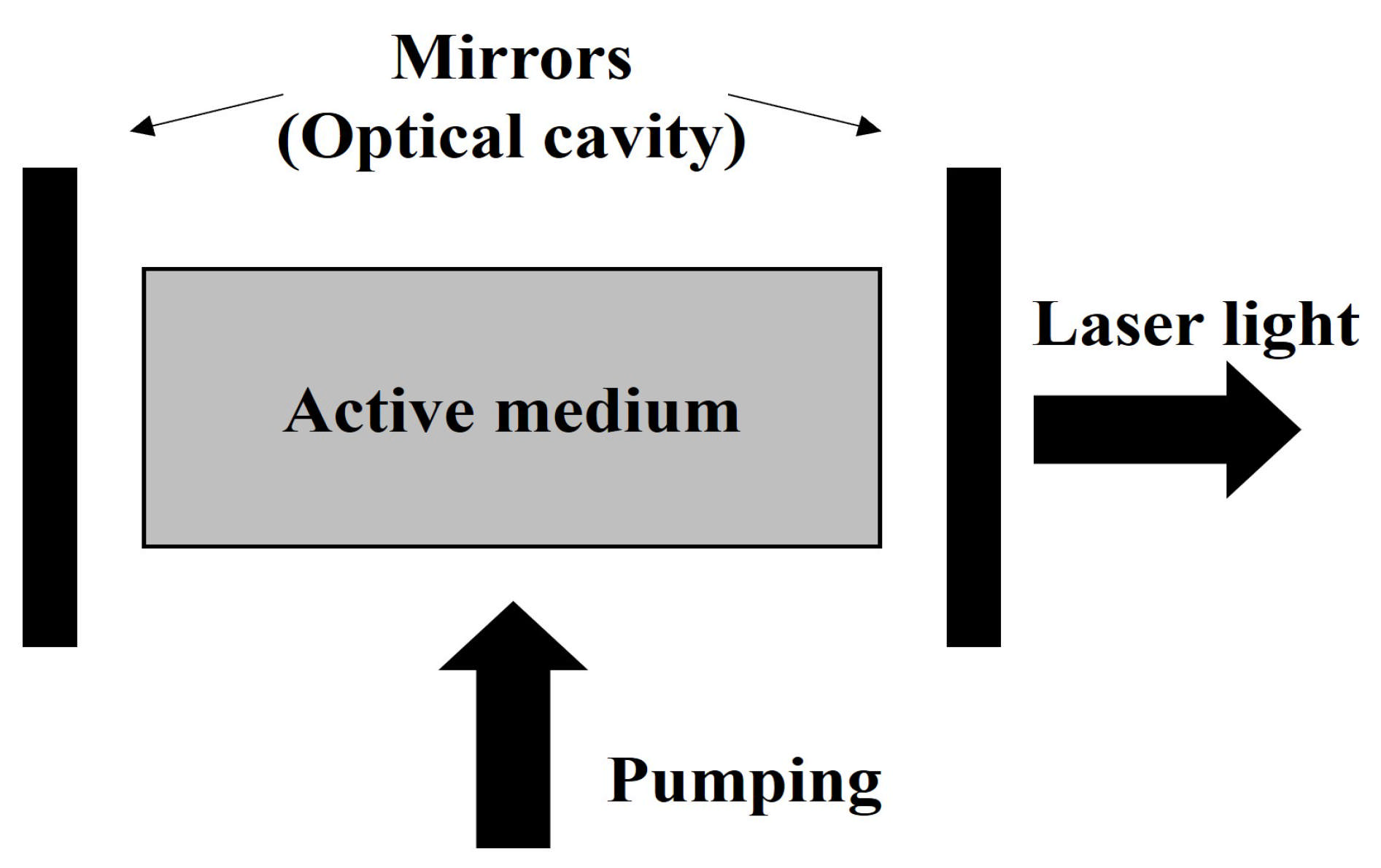
The Maxwell–Bloch equations describe the behavior of atoms at low concentrations, where spectral lines resemble those observed in gases commonly used in dye substances, certain solid-state lasers, and other applications [28]. In general, atomic, molecular, or solid-state media possess an infinite number of energy eigenstates, with spectral lines corresponding to the allowed transitions between pairs of these states (see Figure 6). Since the system can be approximated as a quasi-monochromatic field, only one transition resonates effectively over time, which is typically the transition relevant to laser operation.

Laser emission is governed by processes of stimulated emission occurring between the upper and lower laser energy levels. This fundamental interaction can be modeled using a two-level atomic system, which is mathematically equivalent to a spin-${\displaystyle \frac{1}{2}}$ particle in an external magnetic field. In this analogy, the spin can only align parallel or anti-parallel to the field, corresponding to two discrete energy eigenstates. The interaction between these two atomic levels (or the spin system) and an electromagnetic field is formally described by the Maxwell–Bloch equations.

In the following discussion [29,30], the Maxwell–Bloch equations are derived within a semi-classical framework, where the active medium is treated as an ensemble of quantum oscillators, while the electromagnetic fields are described classically using Maxwell’s equations.

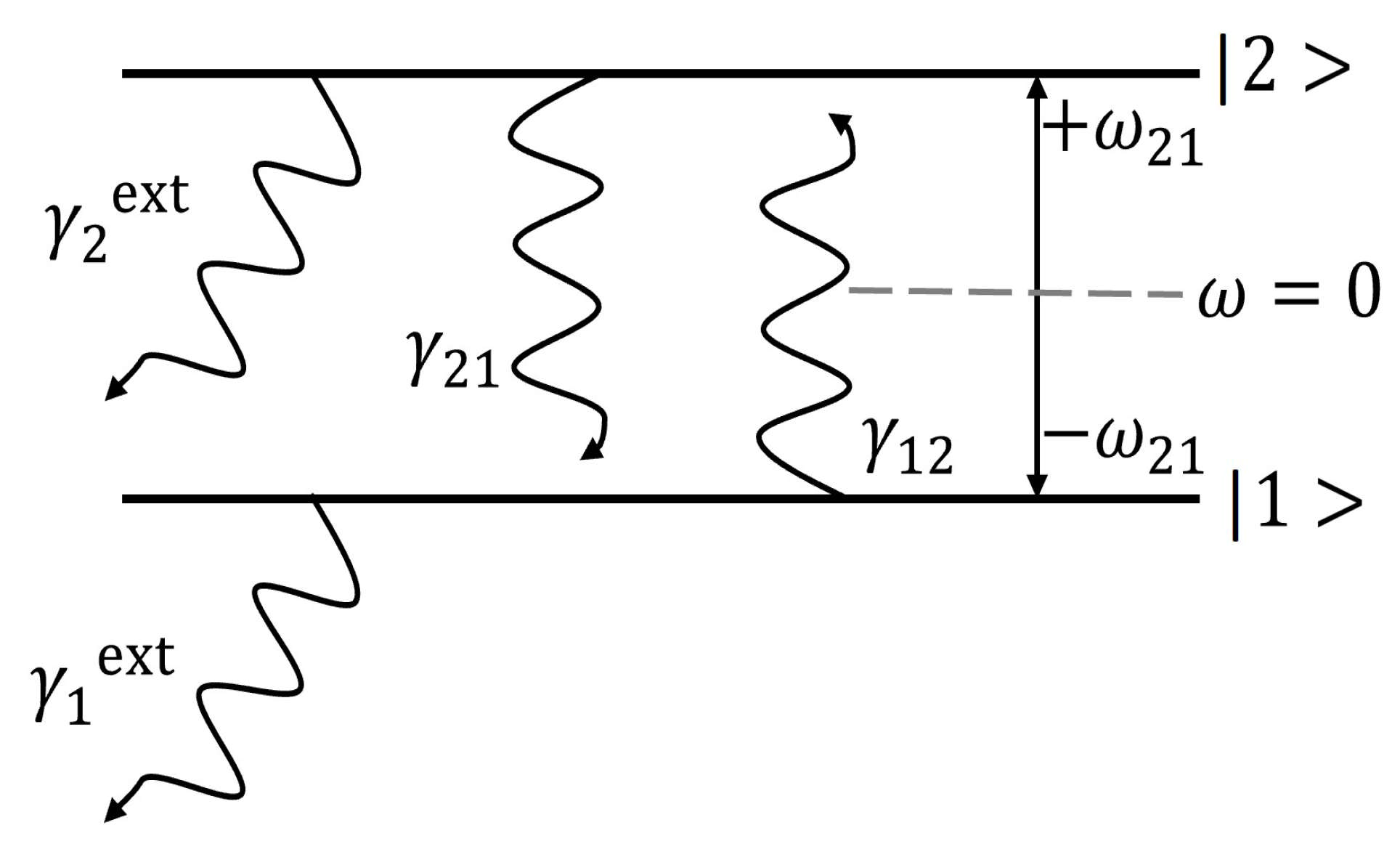
Consider a two-level atomic system interacting with an electromagnetic field. The energy levels are separated by $\Delta E=E_{|2\rangle }-E_{|1\rangle }=\hslash {\omega }_{\alpha }$. When the oscillation frequency of the electric field, $\omega$, matches the transition frequency ${\omega }_{\alpha }$, only the energy states $|1\rangle$ and $|2\rangle$ participate in the interaction (see Figure 7).

The Hamiltonian of the system consists of the unperturbed Hamiltonian and an interaction term, which is given by $H=H_0+H_{int}$.

Both the electric field and polarization can be represented as plane waves propagating along the z axis, which are expressed as

$$\begin{array}{c}\hfill \overrightarrow{E}(z,t)={\displaystyle \frac{1}{2}}\mathcal{E}(z,t)\exp \left[i(kz-\omega t)\right]\widehat{e},\\ \hfill \overrightarrow{P}(z,t)={\displaystyle \frac{1}{2}}\mathcal{P}(z,t)\exp \left[i(kz-\omega t)\right]\widehat{e},\end{array}$$

where $\widehat{e}$ denotes the polarization vector, $k=\omega /c$ is the wave number, and $\omega$ is the carrier frequency.

The fields $\overrightarrow{E}(z,t)$ and $\overrightarrow{P}(z,t)$ satisfy Maxwell’s equations for a nonmagnetic, charge-free medium:

$${\nabla }^2\overrightarrow{E}-{\displaystyle \frac{1}{\sqrt{c}}}{\displaystyle \frac{{\partial }^2\overrightarrow{E}}{\partial t^2}}-\nabla (\nabla ·\overrightarrow{E})={\mu }_0{\displaystyle \frac{{\partial }^2\overrightarrow{P}}{\partial t^2}}.$$

Given that the field amplitudes vary slowly in space and time, their temporal and spatial frequencies are much smaller than the carrier frequency and wave number. This leads to

$${\displaystyle \frac{{\partial }^{2}U}{\partial z^2}}<<k{\displaystyle \frac{\partial U}{\partial z}}<<k^{2}U\mathrm{and}{\displaystyle \frac{{\partial }^{2}U}{\partial t^2}}<<\omega {\displaystyle \frac{\partial U}{\partial t}}<<{\omega }^{2}U,$$

for $U=\mathcal{E}$ and $U=\mathcal{P}$. Consequently, Maxwell’s equation simplifies to Equation (32).

$$\left({\displaystyle \frac{\partial }{\partial t}}+c{\displaystyle \frac{\partial }{\partial z}}\right)\mathcal{E}=i{\displaystyle \frac{\omega }{2{ϵ}_0}}\mathcal{P}$$

(32)

The total Hamiltonian of the system can be written as

$$H=\left(\begin{array}{cc}{\displaystyle \frac{1}{2}}\hslash {\omega }_{21}& V(\overrightarrow{r},t)\\ V^{*}(\overrightarrow{r},t)& -{\displaystyle \frac{1}{2}}\hslash {\omega }_{21}\end{array}\right).$$

The density matrix, which provides information about the medium, is defined as

$$\rho (\overrightarrow{r},t)=\left(\begin{array}{cc}{\rho }_{22}& {\rho }_{21}\\ {\rho }_{12}& {\rho }_{11}\end{array}\right),$$

where the probability that the atom occupies the $|m\rangle$ state is ${\rho }_{mm}$, while ${\rho }_{mn}$ is the coherence between the atomic states. The evolution of $\rho$ is governed by the Schrödinger–von Neumann equation, which is given in terms of the density operator as

$${\displaystyle \frac{d\rho }{dt}}=-{\displaystyle \frac{i}{\hslash }}[H,\rho ].$$

(33)

Substituting the expressions for H, $\rho$, and V into Equation (33), we obtain the set of equations given by Equation (34):

$$\begin{array}{ccc}\hfill {\displaystyle \frac{\partial }{\partial t}}{\rho }_{22}& =& -{\gamma }_2{\rho }_{22}+{\gamma }_{12}{\rho }_{11}+i(\alpha {\sigma }_{12}-{\alpha }^{*}{\sigma }_{21})\hfill \\ \hfill {\displaystyle \frac{\partial }{\partial t}}{\rho }_{11}& =& -{\gamma }_1{\rho }_{11}+{\gamma }_{21}{\rho }_{22}-i(\alpha {\sigma }_{12}-{\alpha }^{*}{\sigma }_{21})\hfill \\ \hfill {\displaystyle \frac{\partial }{\partial t}}{\sigma }_{12}& =& -({\gamma }_{\perp }+i\delta ){\sigma }_{12}+i{\alpha }^{*}({\rho }_{22}-{\rho }_{11})\hfill \end{array}$$

(34)

where the relaxation ratio ${\gamma }_i$ of the $|i\rangle$ level to an external level and ${\gamma }_{ij}$ describes the relaxation ratio of the $|i\rangle$ level to the $|j\rangle$ level. In general, ${\gamma }_{\left|\right|}={\gamma }_i={\gamma }_{ij}$, and ${\gamma }_{\perp }$ is the relaxation ratio for collisions that do not affect the population of atoms.

Let ${\rho }_{ii}$ denote the fraction of atoms occupying the state $|i\rangle$, i.e., the population at this level. The population difference between the two levels is then defined as $d={\rho }_{22}-{\rho }_{11}$, allowing us to rewrite Equation (34) in the form of Equation (35):

$$\begin{array}{ccc}\hfill {\displaystyle \frac{\partial }{\partial t}}d& =& {\gamma }_{\left|\right|}(d_0-d)+2i(\alpha {\sigma }_{12}-{\alpha }^{*}{\sigma }_{21})\hfill \\ \hfill {\displaystyle \frac{\partial }{\partial t}}{\sigma }_{12}& =& -({\gamma }_{\perp }+i\delta ){\sigma }_{12}+i{\alpha }^{*}d\hfill \end{array}$$

(35)

Here, $d_0={\rho }_{22}^0-{\rho }_{11}^0$ represents the initial population difference in the absence of an electromagnetic field, where ${\rho }_{ii}^0$ is the population at level $|i\rangle$.

By combining the field Equation (32) with the matter Equation (35), we obtain a closed system of equations that describe the dynamics of a laser.

Using the expression for polarization, along with Maxwell’s equation (32) and the Bloch equations, the full set of Maxwell–Bloch equations can be written as Equation (36).

$$\begin{array}{ccc}\hfill \left({\displaystyle \frac{\partial }{\partial t}}+c{\displaystyle \frac{\partial }{\partial z}}\right)\alpha & =& ig{\sigma }_{21}\hfill \\ \hfill {\displaystyle \frac{\partial }{\partial t}}{\sigma }_{21}& =& -({\gamma }_{\perp }+i\delta ){\sigma }_{12}+i{\alpha }^{*}d\hfill \\ \hfill {\displaystyle \frac{\partial }{\partial t}}d& =& -{\gamma }_{\left|\right|}(d_0-d)+2i(\alpha {\sigma }_{12}-{\alpha }^{*}{\sigma }_{21})\hfill \end{array}$$

(36)

where $g=N\omega |{\overrightarrow{\mu }}_{12}{·e|}^2/2{ϵ}_0\hslash$ is the coupling constant between radiation and matter, determining the interaction strength between the field and the medium.

For uniform fields with appropriate boundary conditions, the Maxwell–Bloch equations are reduced to the following form:

$$\begin{array}{ccc}\hfill {\displaystyle \frac{\partial F}{\partial t}}+v{\displaystyle \frac{\partial F}{\partial z}}& =& \kappa (P-F)\hfill \\ \hfill {\displaystyle \frac{\partial P}{\partial t}}& =& {\gamma }_{\perp }(FD-P)\hfill \\ \hfill {\displaystyle \frac{\partial D}{\partial t}}& =& {\gamma }_{\left|\right|}(r-D-{\displaystyle \frac{1}{2}}(F{P}^{*}+F^{*}P))\hfill \end{array}$$

where

$$F(z,t)={\displaystyle \frac{2}{\sqrt{{\gamma }_{\left|\right|}{\gamma }_{\perp }}}}{\alpha }^{\prime }(z,t),D(z,t)={\displaystyle \frac{r}{d_0}}{d}^{\prime }(z,t)$$

and

$$P(z,t)=2i{\displaystyle \frac{r}{d_0}}\sqrt{{\displaystyle \frac{{\gamma }_{\perp }}{{\gamma }_{\left|\right|}}}}{\sigma }_{21}^{\prime }(z,t).$$

Next, for a single-mode laser in resonance ${\Delta }_c=0,{\displaystyle \frac{\partial F}{\partial z}}=0$. Then, the field F and the atomic polarization P can be expressed as $F=Eexp\left[i\varphi \right]$ and $P=(P_{re}+i{P}_{im}exp\left[i\varphi \right])$, where the electric field E is a real quantity. Using these definitions, Equations (37)–(40) are introduced.

$$\dot{E}=\kappa (P_{re}-E)$$

(37)

$$\dot{\varphi }=\kappa {\displaystyle \frac{P_{im}}{E}}$$

(38)

$$\dot{P_{re}}={\gamma }_{\perp }(ED-P_{re})+\dot{\varphi }{P}_{im}$$

(39)

$$\dot{P_{im}}=-{\gamma }_{\perp }{P}_{im}-\dot{\varphi }{P}_{re}$$

(40)

From Equations (37) and (39), the Equation (41) is obtained as

$${\displaystyle \frac{\dot{P_{im}}}{P_{im}}}+{\displaystyle \frac{\dot{E}}{E}}=-(k+{\gamma }_{\perp })$$

(41)

Consequently, Equation (41) implies that the imaginary part vanishes, as shown in Equation (42):

$$P_{im}\left(t\right)={\displaystyle \frac{P_{im}\left(0\right)}{E\left(0\right)}}E\left(t\right)exp[-(k+{\gamma }_{\perp })]\to 0$$

(42)

Applying the result of Equation (42) to Equation (38) leads to $\dot{\varphi }\to 0$.

Finally, the variable change is applied as

$$X=E,Y=p,Z=r-D,\sigma ={\displaystyle \frac{\kappa }{{\gamma }_{\perp }}}\mathrm{and}b={\displaystyle \frac{{\gamma }_{\left|\right|}}{{\gamma }_{\perp }}}$$

and the resulting equations are shown in Equation (43):

$$\begin{array}{ccc}\hfill {\displaystyle \frac{\partial X}{\partial \tau }}& =& -\sigma X+\sigma Y\hfill \\ \hfill {\displaystyle \frac{\partial Y}{\partial \tau }}& =& -Y+rX+XZ\hfill \\ \hfill {\displaystyle \frac{\partial Z}{\partial \tau }}& =& bZ-bXY\hfill \end{array}$$

(43)

5. The Gyrostat

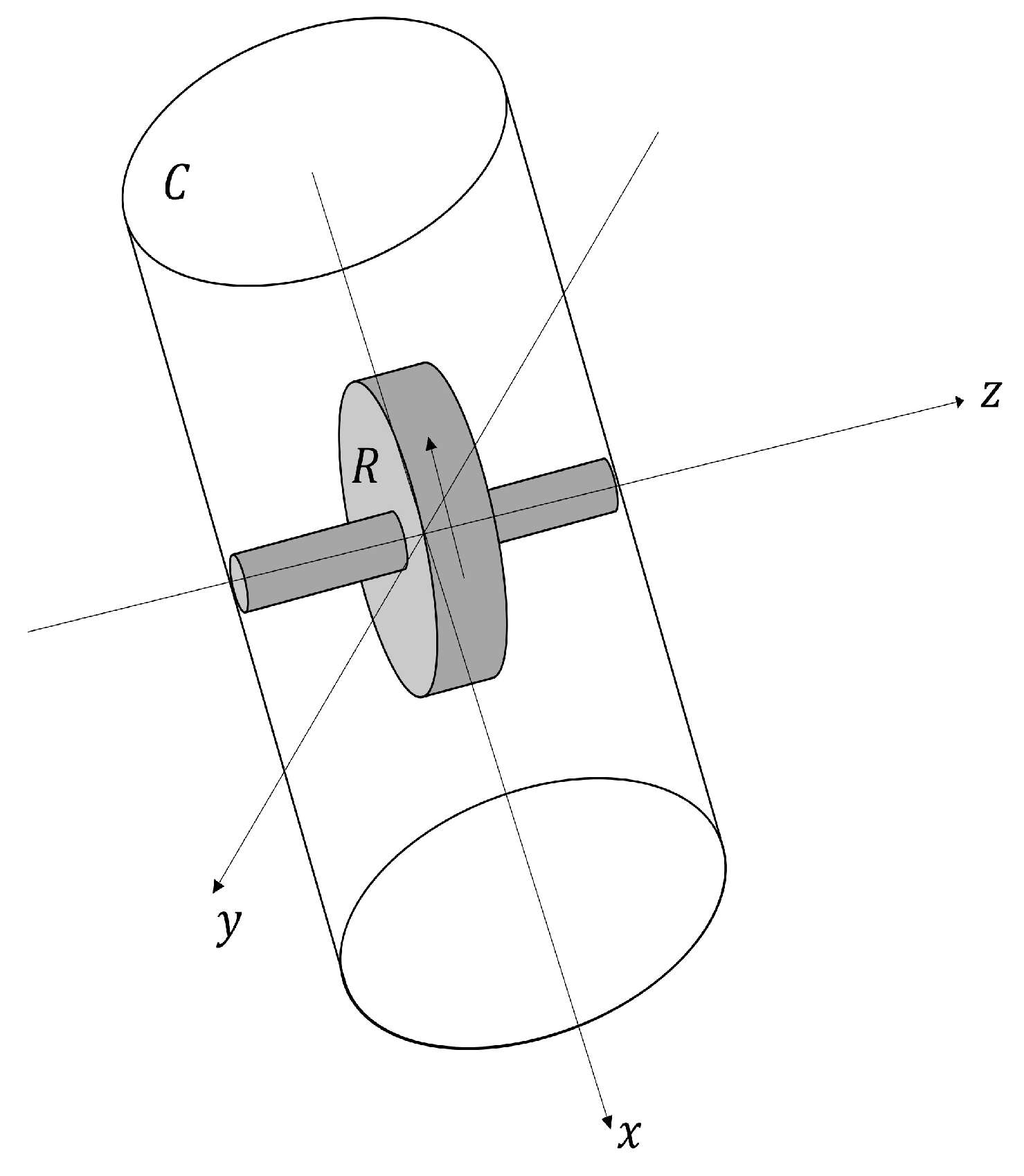
Another mechanical system described by a set of differential equations equivalent to the Lorenz equations was studied by Zlochevsky [31,32,33,34]. This inertial mechanical system consists of two solid bodies: a cylindrical body, denoted as B, which rotates around its own axis in the x direction, and a rotor R with axial symmetry, which rotates around the z axis within the body C (see Figure 8).

In the description of the system, it is assumed that the center of mass remains fixed at both the center of the cylinder and the rotor. Additionally, the inertia ellipsoid is considered to be a body of revolution, meaning that $I_y=I_z=I$, where $I_y$ and $I_z$ are the moments of inertia along the y and z axes, respectively.

The rotor rotates with a constant angular velocity $\Omega$ around its symmetry axis z, which is fixed within the cylinder and undergoes transverse rotation around the x axis. The torque $\overrightarrow{M}$ acting on the gyrostat depends on the angular velocity $\omega$ of the system, which includes both the cylinder and the rotor, rotating around the fixed center of mass. Thus, the angular momentum of the gyrostat is given by Equation (44):

$$\overrightarrow{L}=I·\overrightarrow{w},$$

(44)

where I represents the inertia matrix relative to the given set of axes, and $\overrightarrow{\omega }$ is a pseudo-vector perpendicular to the plane of rotation. It is worth noting that in Equation (44), the symbol “·” denotes the conventional multiplication between the inertia matrix I and the pseudo-vector $\overrightarrow{\omega }$.

Since these axes are fixed with respect to the rotating body, they rotate with the reference frame. Consequently, the angular momentum can be expressed as

$$\overrightarrow{L}=(I_x{\omega }_x,I_y{\omega }_y,I_z{\omega }_z),$$

where ${\omega }_x$, ${\omega }_y$, and ${\omega }_z$ are the components of the angular velocity $\omega$ along the principal axes. These correspond to the projections of the vector $\overrightarrow{L}$ at a given instant in space onto the principal axes.

The torque acting on the system is defined as the time derivative of the angular momentum. For this two-body system, it follows that

$$\overrightarrow{M}={\left({\displaystyle \frac{d\overrightarrow{L}}{dt}}\right)}_{in}={\left({\displaystyle \frac{d\overrightarrow{L}}{dt}}\right)}_{lab}+{\left(\overrightarrow{\omega }\times \overrightarrow{L}\right)}_C+{\left(\overrightarrow{\omega }\times \overrightarrow{N}\right)}_R$$

where the first term represents the rate of change of angular momentum in the reference frame of the gyrostat, the second term accounts for the rate of change in the body frame, and the last term corresponds to the torque exerted by the rotor R, whose angular momentum is given by Equation (45):

$$\overrightarrow{N}=J·\overrightarrow{\Omega }=(0,0,J_z{\Omega }_z),$$

(45)

where J is the moment of inertia associated with the rotor. Since the rotor rotates around the z axis, the components of the vector $\overrightarrow{N}$ satisfy $N_x=N_y=0$, meaning only the z component is nonzero. In other words, the following magnitudes are equal, and we have $|\overrightarrow{N}|=|N_z|$.

In this way, the torque acting on the system is given as Equation (46):

$$\begin{array}{ccc}\hfill \overrightarrow{M}& =& (I_x{\dot{\omega }}_x,I_y{\dot{\omega }}_y,I_z{\dot{\omega }}_z)\hfill \\ & +& (0,(I_x-I_z){\omega }_x{\omega }_z,(I_y-I_x){\omega }_y{\omega }_x)\hfill \\ & +& ({\omega }_y{N}_z,-{\omega }_x{N}_z,0)\hfill \end{array}$$

(46)

where the dot indicates differentiation with respect to time.

By decomposing the vector equation $\overrightarrow{M}=(M_x,M_y,M_z)$ into its components, we obtain the following system of differential equations given by Equation (47):

$$\begin{array}{ccc}\hfill M_x& =& I_x{\dot{\omega }}_x+N_z{\omega }_y\hfill \\ \hfill M_y& =& I_y{\dot{\omega }}_y+(I_x-I_z){\omega }_x{\omega }_z-N_z{\omega }_x\hfill \\ \hfill M_z& =& I_z{\dot{\omega }}_z+(I_y-I_x){\omega }_y{\omega }_x\hfill \end{array}$$

(47)

For $M_x=M_y=M_z=0$, with $\omega \ne 0$ and $\Omega \ne 0$, the gyrostat exhibits periodic or permanent rotational motion. These movements correspond to specific trajectories in the phase space for the system at equilibrium.

If $M_x$, $M_y$, and $M_z$ are nonzero and satisfy $M_x=(N_1+N_z){\omega }_y-N_1{\omega }_x$, $M_y=-N_2{\omega }_y$, and $M_z=-N_3{\omega }_z$, then the system in Equation (47) can be rewritten as Equation (48):

$$\begin{array}{ccc}\hfill I_x{\dot{\omega }}_x& =& N_1({\omega }_y-{\omega }_x)\hfill \\ \hfill I_y{\dot{\omega }}_y& =& N_z{\omega }_x-(I_x-I){\omega }_x{\omega }_z-N_2{\omega }_y\hfill \\ \hfill I_z{\dot{\omega }}_z& =& (I_x-I){\omega }_y{\omega }_x-N_3{\omega }_z\hfill \end{array}$$

(48)

where $N_1$, $N_2$, and $N_3$ are coefficients related to the moment of inertia of the rotor. By introducing the variable transformations

$$X={\displaystyle \frac{(I_x-I){\omega }_x}{N_2}},Y={\displaystyle \frac{(I_x-I){\omega }_y}{N_2}},Z={\displaystyle \frac{(I_x-I){\omega }_z}{N_2}}$$

and

$$\tau ={\displaystyle \frac{N_2}{I}}t,\sigma ={\displaystyle \frac{N_{1}I}{N_2{I}_x}},b={\displaystyle \frac{N_3}{N_2}}$$

we obtain a system of differential equations equivalent to the standard Lorenz equations, as given by Equation (49):

$$\begin{array}{ccc}\hfill \dot{X}& =& -\sigma X+\sigma Y\hfill \\ \hfill \dot{Y}& =& -Y+rX-XZ\hfill \\ \hfill \dot{Z}& =& -bZ+XY\hfill \end{array}$$

(49)

6. Solar Dynamo Model

Observations of solar and stellar phenomena frequently reveal variations arising from the dynamics of hydromagnetic processes. Extensive studies have been conducted using magnetohydrodynamics equations to describe solar and stellar dynamos, which are inherently complex systems. As a result, an entire formal framework has been developed within the field of dynamo theory. Furthermore, research on solar dynamo behavior has focused on analyzing solar variability [35,36,37,38].

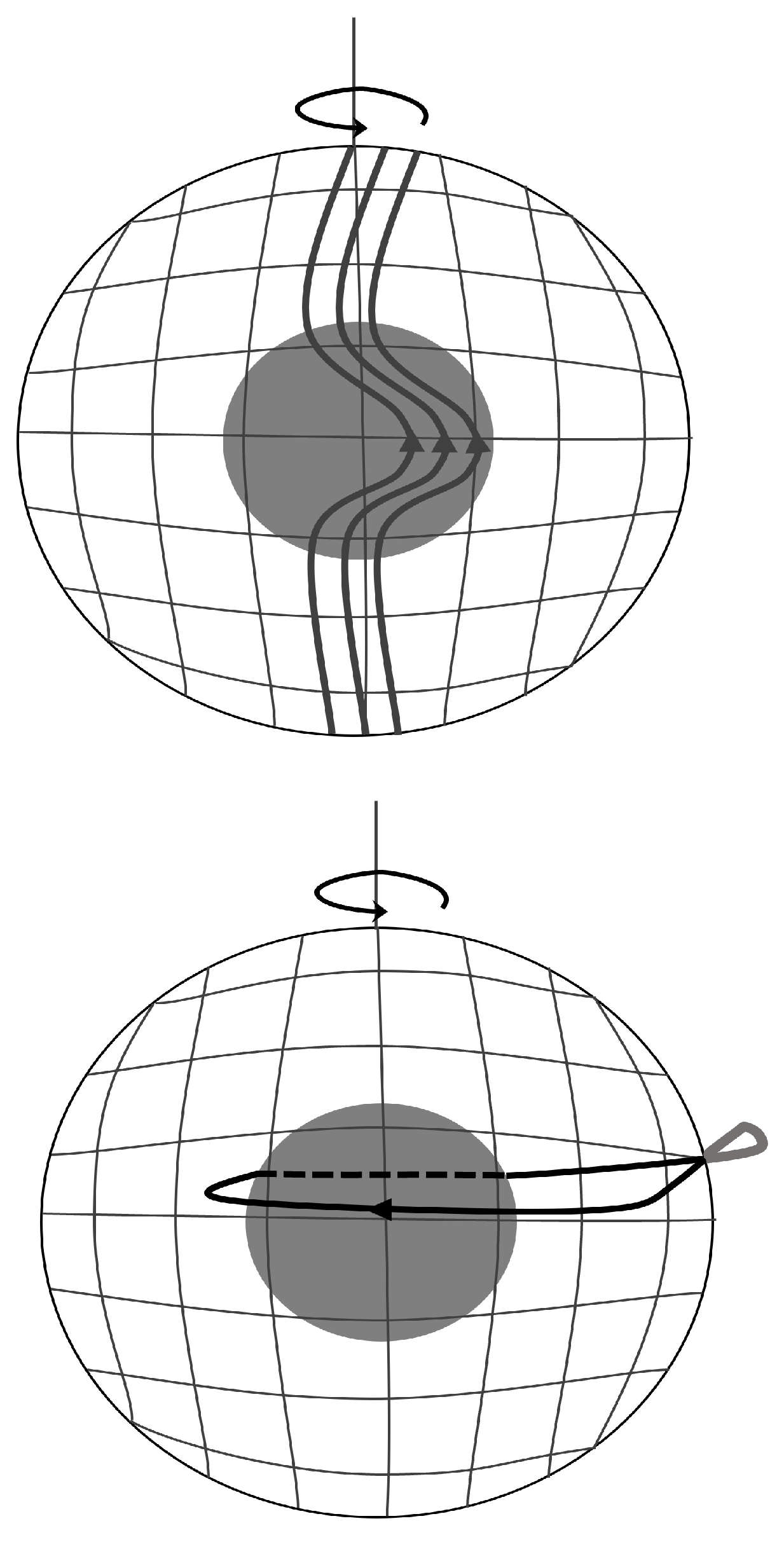
This phenomenon can be qualitatively understood by considering magnetic field lines as elastic bands subjected to magnetic tension and pressure (see Figure 9). These fields can be intensified through various deformations, such as stretching, twisting, and bending. Such distortions are primarily induced by plasma motion within the convection zone and largely governed by the $\alpha$ effect, where ascending convection flows twist magnetic field lines in combination with the Coriolis force.

The dynamics of $\alpha$ models begin with the magnetic field induction equation, presented in Equation (50), that has been previously studied [35,36,37,38].

$${\displaystyle \frac{\partial \overrightarrow{B}}{\partial t}}=\nabla \times (\overrightarrow{v}\times \overrightarrow{B}+\alpha \overrightarrow{B}-{\eta }_t\nabla \times \overrightarrow{B})$$

(50)

where $\overrightarrow{B}$ represents the magnetic field, and $\overrightarrow{v}$ denotes the flow velocity. The term ${\eta }_t$ corresponds to the turbulent magnetic diffusivity, while the $\alpha$ coefficient links the electric current generated by helical turbulence (the $\alpha$ effect) to the magnetic field, both of which emerge from small-scale turbulent correlations between velocity and magnetic fields.

For a configuration in which the spatial coordinate x corresponds to latitude, and assuming a longitudinal velocity with a constant radial gradient and a vertical component ${\omega }_0$, the magnetic field can be expressed as

$$\overrightarrow{B}=\left(0,B_{\varphi },{\displaystyle \frac{1}{R}}{\displaystyle \frac{\partial A_{\varphi }}{\partial x}}\right)$$

where $A_{\varphi }$ represents the longitudinal component of the magnetic potential, $B_{\varphi }$ is the azimuthal component of $\overrightarrow{B}$, and x is measured in units of stellar radius. Under these conditions, the governing equations take the form

$$\begin{array}{ccc}\hfill {\displaystyle \frac{\partial A_{\varphi }}{\partial t}}& =& {\displaystyle \frac{{\eta }_t}{R^2}}{\displaystyle \frac{{\partial }^2{A}_{\varphi }}{\partial x^2}}+\alpha B_{\varphi }\hfill \\ \hfill {\displaystyle \frac{\partial B_{\varphi }}{\partial t}}& =& {\displaystyle \frac{{\eta }_t}{R^2}}{\displaystyle \frac{{\partial }^2{B}_{\varphi }}{\partial x^2}}+{\displaystyle \frac{{\omega }_0}{R}}{\displaystyle \frac{\partial A_{\varphi }}{\partial x}}\hfill \end{array}$$

The $\alpha$ coefficient consists of both a static (kinematic) and a dynamic (magnetic) component, given by $\alpha ={\alpha }_{0}cosx-{\alpha }_{M}t$, where the time-dependent part evolves according to

$${\displaystyle \frac{\partial {\alpha }_M}{\partial t}}=▵\left({\alpha }_M\right)+f(\overrightarrow{B}),$$

where △ is a damping operator, and $f(\overrightarrow{B})$ is a quadratic function of the magnetic field, which is generally expressed as

$$f(\overrightarrow{B})=W_1\overrightarrow{J}·\overrightarrow{B}+W_2\alpha {|\overrightarrow{B}|}^2,$$

where $W_1$ and $W_2$ are constants, and $\overrightarrow{J}$ represents the electric current.

To derive a dimensionless formulation, we introduce a reference field $B_0$, measure time in units of $R^2/{\eta }_t$, and define the following nondimensional variables:

$$A={\displaystyle \frac{R{\omega }_0}{B_0{\eta }_t}}{A}_{\varphi },B={\displaystyle \frac{B_{\varphi }}{B_0}},C={\displaystyle \frac{{\alpha }_M{R}^3{\omega }_0}{{\eta }_t^2}}$$

$$v={\displaystyle \frac{v_t}{{\eta }_t}}\mathrm{and}D={\displaystyle \frac{{\alpha }_0{\omega }_0{R}^3}{{\eta }_t^2}}$$

where $v_t$ is the turbulent diffusivity, and the operator is defined as

$$▵={\displaystyle \frac{v_t}{R^2}}{\displaystyle \frac{{\partial }^2}{\partial x^2}}.$$

Thus, the system of equations can be rewritten in nondimensional form as

$$\begin{array}{ccc}\hfill {\displaystyle \frac{\partial A}{\partial t}}& =& {\displaystyle \frac{{\partial }^{2}A}{\partial x^2}}+DBcosx-CB\hfill \\ \hfill {\displaystyle \frac{\partial B}{\partial t}}& =& {\displaystyle \frac{{\partial }^{2}B}{\partial x^2}}+{\displaystyle \frac{\partial A}{\partial x}}\hfill \\ \hfill {\displaystyle \frac{\partial C}{\partial t}}& =& v{\displaystyle \frac{{\partial }^{2}C}{\partial x^2}}+AB.\hfill \end{array}$$

By considering the interval $0\le x\le \pi$, which encompasses the full range of latitudes, and imposing the boundary conditions $A=B=C=0$ at $x=0$ and $x=\pi$, we apply a spectral expansion as follows:

$$A=\sum _{n=1}^N{A}_n\left(t\right)sin\left[nx\right],B=\sum _{n=1}^N{B}_n\left(t\right)sin\left[nx\right]$$

and

$$C=\sum _{n=1}^N{C}_n\left(t\right)sin\left[nx\right]$$

which leads to the reformulation of the system as

$$\begin{array}{ccc}\hfill {\displaystyle \frac{\partial A_1}{\partial t}}& =& -A_1+{\displaystyle \frac{D{B}_2}{2}}-{\displaystyle \frac{32B_2{C}_2}{15\pi }}\hfill \\ \hfill {\displaystyle \frac{\partial B_2}{\partial t}}& =& -4B_2+{\displaystyle \frac{8A_1}{3\pi }}\hfill \\ \hfill {\displaystyle \frac{\partial C_2}{\partial t}}& =& -4v{C}_2+{\displaystyle \frac{16A_1{B}_2}{5\pi }}.\hfill \end{array}$$

By introducing the new variables

$$A_1={\displaystyle \frac{15\sqrt{6}{\pi }^2}{64}}Y,B_2={\displaystyle \frac{5\sqrt{6}\pi }{32}}X,C_2={\displaystyle \frac{45{\pi }^2}{64}}Z$$

the resulting equations become equivalent to the Lorenz system, which is expressed in Equation (51).

$$\begin{array}{ccc}\hfill {\displaystyle \frac{dX}{dt}}& =& -\sigma X+\sigma Y\hfill \\ \hfill {\displaystyle \frac{dY}{dt}}& =& -Y+rX-XZ\hfill \\ \hfill {\displaystyle \frac{dZ}{dt}}& =& -bZ+XY,\hfill \end{array}$$

(51)

where the control parameters are given by $\sigma =4$, $b=4v$, and $r=D/3\pi$.

For numerous astrophysical contexts, including solar dynamics, the sign of the dynamo number remains uncertain, and it is crucial to analyze the system’s behavior before any sign changes occur. Furthermore, the value of D must remain below a specific threshold to ensure that numerical solutions to Equation (51) remain convergent.

7. Mesoscopic Dynamics in Chemical Reactions

Nonlinear phenomena in chemical reactions, such as periodic and aperiodic sustained oscillations, are frequently observed in solution-phase, gas-phase, and heterogeneous reactions occurring in continuously stirred tank reactors [39].

Numerous reaction models exhibit nonlinear chemical kinetics, relying on macroscopic equations derived from kinetic postulates. However, from a microscopic or mesoscopic perspective, the self-organization behaviors of these systems originate from random molecular collisions and stochastic processes. Therefore, understanding mesoscopic dynamics is essential to accurately describe experimental observations and develop robust macroscopic models.

The Fokker–Planck equation is commonly employed to characterize various mesoscopic-scale phenomena. However, for complex systems such as chemical reactions, solving this equation analytically is highly challenging and, in many cases, infeasible. Consequently, numerical studies are often conducted to analyze the behavior of these systems.

In the following section, the microscopic dynamics of a chemical Lorenz system are examined using a mesoscopic-scale approach based on the Fokker–Planck equation [40]. This chemical system is inspired by the original Lorenz model and its distinctive nonlinear behavior, wherein macroscopic dynamics exist within a chaotic regime [41,42].

A chemical reaction scheme capable of reproducing the original Lorenz system dynamics can be constructed by considering the following sequence of reactions, as presented in Equation (52) [40]:

$$\begin{array}{ccc}\hfill R_1:X+Y+Z& {⟶}^{k_1}& X+2Z\hfill \\ \hfill R_2:A_1+X+Y& {⟶}^{k_2}& 2X+Y\hfill \\ \hfill R_3:A_2+X+Y& {⟶}^{k_3}& X+2Y\hfill \\ \hfill R_4:X+Z& {⟶}^{k_4}& X+P_1\hfill \\ \hfill R_5:Y+Z& {⟶}^{k_5}& 2Y\hfill \\ \hfill R_6:2X& {⟶}^{k_6}& P_2\hfill \\ \hfill R_7:2Y& {⟶}^{k_7}& P_3\hfill \\ \hfill R_8:2Z& {⟶}^{k_8}& P_4\hfill \\ \hfill R_9:A_3+X& {⟶}^{k_9}& 2X\hfill \\ \hfill R_{10}:X& {⟶}^{k_{10}}& P_5\hfill \\ \hfill R_{11}:Y& {⟶}^{k_{11}}& P_6\hfill \\ \hfill R_{12}:A_4+Y& {⟶}^{k_{12}}& 2Y\hfill \\ \hfill R_{13}:A_5+Z& {⟶}^{k_{13}}& 2Z\hfill \end{array}$$

(52)

where coefficients $k_i$ ($i=1,2,\dots ,13$) represent rate constants, while the concentrations of species $A_i$ ($i=1,2,\dots ,5$) characterize an out-of-equilibrium system. From a mesoscopic perspective, this reaction scheme can be treated as a discrete Markov process, provided that the system is well mixed and maintains local equilibrium.

The system’s dynamics are described by the Fokker–Planck master equation, which describes the evolution of the probability density function $P(\overrightarrow{r},t)$. This equation is given by Equation (53):

$${\displaystyle \frac{\partial }{\partial t}}P(\overrightarrow{r},t)=\int \left(w\left(\overrightarrow{r}\right|{\overrightarrow{r}}^{\prime })P({\overrightarrow{r}}^{\prime },t)-w\left({\overrightarrow{r}}^{\prime }\right|\overrightarrow{r})P(\overrightarrow{r},t)\right)d{\overrightarrow{r}}^{\prime },$$

(53)

where $w\left(\overrightarrow{r}\right|{\overrightarrow{r}}^{\prime })$ is the transition probability per unit of time from state $\overrightarrow{r}=(x,y,z)$ to state ${\overrightarrow{r}}^{\prime }$. This yields a set of differential equations governing the concentrations of species x, y, and z, as shown in Equation (54):

$$\begin{array}{ccc}\hfill {\displaystyle \frac{dx}{dt}}& =& k_{2}xy-2k_6{x}^2+k_{9}x-k_{10}x\hfill \\ \hfill {\displaystyle \frac{dy}{dt}}& =& -k_{1}xyz+k_{3}xy+k_{5}yz-2k_7{y}^2-k_{11}y+k_{12}y\hfill \\ \hfill {\displaystyle \frac{dz}{dt}}& =& k_{1}xyz-k_{4}xz-k_{5}yz-2k_8{z}^2+k_{13}z.\hfill \end{array}$$

(54)

By applying an appropriate transformation, commonly used in dynamical studies of mechanical and electrical systems, the above equations of Equation (55) can be rewritten in a form equivalent to the original Lorenz system:

$$\begin{array}{ccc}\hfill \dot{x}& =& -\sigma (x-y)\hfill \\ \hfill \dot{y}& =& -xz+rx-y\hfill \\ \hfill \dot{z}& =& xy-bz,\hfill \end{array}$$

(55)

where the parameters $\sigma$, r, and b are positive constants, and the variables x, y, and z can take arbitrary values depending on the system under study. However, in the context of the chemical system, both the parameters $k_i$ and the variables x, y, and z are strictly non-negative.

8. Interest Rate Model

Different models exist in this field, many of which are stochastic and capable of describing the behavior of interest rates. However, these models have primarily been developed to represent the static and dynamic characteristics of structural terms rather than to depict interest rates as the outcome of a fundamental economic process [43]. In this context, extensive research has been conducted using the general economic equilibrium model, while other studies have explored approaches beyond equilibrium models. This study presents an interest rate model that, while not entirely based on the general equilibrium framework, incorporates essential economic principles [44].

The following description provides only a general overview and is not intended to be highly detailed. For a more comprehensive explanation, please refer to [45].

This model, which focuses on short-term interest rates, aims to provide a natural explanation of the behavior of this economic variable. The dynamics of the short-term interest rate can be expressed in the following general form of Equation (56):

$$\begin{array}{ccc}\hfill dr& =& \alpha (x-r)dt+{\sigma }_{r}d{z}_r\hfill \\ \hfill dx& =& \beta ({\mu }_x(t,r,Y)-x)dt+{\sigma }_{x}d{z}_x\hfill \\ \hfill dY& =& \gamma ({\mu }_Y(t,r,x,Y)-Y)dt+{\sigma }_{Y}d{z}_Y.\hfill \end{array}$$

(56)

This model explains the evolution of the short-term interest rate, where r represents the short-term interest rate, x denotes the reference level to which the short rate adjusts, and Y is a vector capturing residual effects of the model’s dynamics through the function ${\mu }_x$. The parameters $\alpha$, $\beta$, and $\gamma$ serve as weighting coefficients. Thus, the interest rate over time is expressed as a weighted difference between the feedback level x and the actual rate r, in addition to a volatility term $({\sigma }_r,{\sigma }_x,{\sigma }_Y)$. Similarly, the temporal values of x and Y are determined by their respective weighted differences and volatility components.

Furthermore, multiple studies have explored the influence of monetary policy (monetary flow) on short-term interest rate behavior [46].

The IS-LM model, like other economic models, is represented by equilibrium equations. In this case, the two state variables are $X=(r,y)$, where r is the short-term real interest rate, and y is the real national income rate. In addition, the dynamics of the state variables can be expressed as Equation (57) [44].

$$dX=B^{-1}A\left((C-B)X+(\underline{c}-\underline{b})\right)dt+B^{-1}\Sigma dz.$$

(57)

In addition, two affine functions of the state variables X are defined in Equation (58) as

$$\begin{array}{cc}\hfill M& =BX+\underline{b},\hfill \\ \hfill \overline{M}& =CX+\underline{c},\hfill \end{array}$$

(58)

On the other hand, the two corresponding equilibrium conditions are derived from the sum of the money supply $m_s$ and money demand $m_d$, as well as from the relationship between the real national income rate y and real national expenditure e. These variables are linked by the Equation (59).

$$\begin{array}{cc}\hfill m_d& =ky-ur,\hfill \\ \hfill e& =a-br+cy,\hfill \end{array}$$

(59)

where $u,k,a,b,c>0$, and $0<c<1$.

In the IS-LM framework B, C, $\underline{b}$, and $\underline{c}$ are defined in Equation (60); as well, $M=(m_d,y)$, and $\overline{M}=(m_s,e)$.

$$B=\left(\begin{array}{cc}-u& k\\ 0& 1\end{array}\right),C=\left(\begin{array}{cc}0& 0\\ -b& c\end{array}\right),b=\left(\begin{array}{c}0\\ 0\end{array}\right),c=\left(\begin{array}{c}{m}_s\\ a\end{array}\right),$$

(60)

and also, $\Sigma$ and A are defined in Equation (61).

$$\Sigma =\left(\begin{array}{cc}{\sigma }_m& 0\\ 0& {\sigma }_y\end{array}\right),A=\left(\begin{array}{cc}{\alpha }_m& 0\\ 0& {\alpha }_y\end{array}\right).$$

(61)

where ${\alpha }_m$ is the rate of adjustment in the money market and is large; ${\alpha }_y$ is the rate of adjustment in the goods market and is small.

By substituting Equations (60) and (61) into Equation (57), we obtain Equation (62), which describes the dynamics of y and r. The definitions of the remaining variable changes in the substitution are provided in Equation (63).

$$\begin{array}{cc}\hfill dr& =v\left({\displaystyle \frac{q}{v}}+{\displaystyle \frac{w}{v}}y-r\right)dt+{\sigma }_{r}d{z}_r,\hfill \\ \hfill dy& ={\alpha }_y(1-c)\left({\displaystyle \frac{a}{1-c}}-{\displaystyle \frac{b}{1-c}}r-y\right)dt+{\sigma }_{y}d{z}_y,\hfill \end{array}$$

(62)

$$\begin{array}{cc}\hfill q& =a{\alpha }_y{\displaystyle \frac{k}{u}}-{\alpha }_m{\displaystyle \frac{m_s}{u}},v={\alpha }_m+{\alpha }_{y}b{\displaystyle \frac{k}{u}},w={\alpha }_m{\displaystyle \frac{k}{u}}-{\alpha }_y(1-c){\displaystyle \frac{k}{u}},\hfill \\ \hfill {\sigma }_r^2& ={\displaystyle \frac{1}{u^2}}\left({\sigma }_m^2+k^2{\sigma }_y^2\right)\hfill \end{array}$$

(63)

Next, by applying the variable changes from Equation (64) into Equation (62), Equation (65) is obtained, which characterizes the behavior of r as a function of x. In this case, x represents the expected value of the interest rate, implicitly characterizing the economy.

$${\sigma }_x={\displaystyle \frac{w}{v}}{\sigma }_y,z_x=z_y,x={\displaystyle \frac{q}{v}}+{\displaystyle \frac{w}{v}},p=-{\displaystyle \frac{w}{v}}·{\displaystyle \frac{b}{1-c}},\mu ={\displaystyle \frac{{\displaystyle \frac{a}{1-c}}+{\displaystyle \frac{u}{w}}}{{\displaystyle \frac{b}{1-c}}+{\displaystyle \frac{v}{w}}}}$$

(64)

$$\begin{array}{cc}\hfill dr& =\nu (x-r)dt+{\sigma }_{r}d{z}_r,\hfill \\ \hfill dx& =q(1-c)\left({\displaystyle \frac{w}{\nu }}·{\displaystyle \frac{a}{1-c}}+{\displaystyle \frac{{\alpha }_y}{\nu }}-{\displaystyle \frac{w}{\nu }}·{\displaystyle \frac{b}{1-c}}r-x\right)dt+{\sigma }_{x}d{z}_x\hfill \end{array}$$

(65)

Now, by defining $\alpha =v$ and $\beta ={\alpha }_y(1-c)$, the system represented by Equation (65) can be rewritten as Equation (66):

$$\begin{array}{cc}\hfill dr& =\alpha (x-r)dt+{\sigma }_{r}d{z}_r\hfill \\ \hfill dx& =\beta \left(pr+(1-p)\mu -x\right)dt+{\sigma }_{x}d{z}_x\hfill \end{array}$$

(66)

In this two-factor model, p represents the influence of r on the expected level of x, measuring the degree of feedback between the interest rate and the broader economy. While p is treated as constant within this model in practice, its value is influenced by the aggregate behavior of economic agents.

By introducing the dynamics of p into the system described by Equation (66), i.e., p is no longer constant, a three-factor model is obtained. The third equation is represented by Equation (67):

$$dp=\gamma (\overline{p}-p)dt+{\sigma }_{p}d{z}_p,$$

(67)

where $\overline{p}$ is the equilibrium value of p, and $\gamma$ represents the reversion rate between p and $\overline{p}$. It is possible to expanded $\overline{p}$ in a Taylor series around the fixed point $r_0=u,x_0=u$, as shown in Equation (68):

$$\begin{array}{cc}\hfill \overline{p}(r,x)& =\overline{p}(\mu ,\mu )+{\overline{p}}_r(r-\mu )+{\overline{p}}_x(x-\mu )\hfill \\ \hfill & +{\displaystyle \frac{1}{2}}{\overline{p}}_{rr}{(r-\mu )}^2+{\displaystyle \frac{1}{2}}{\overline{p}}_{xx}{(x-\mu )}^2\hfill \\ \hfill & +{\overline{p}}_{xr}(x-\mu )(r-\mu )+\dots \hfill \end{array}$$

(68)

The next step involves truncating this Taylor series to a second-order approximation. Let $\delta =\overline{p}(\mu ,\mu )$, and define $-\varphi ={\overline{p}}_{xr}$ evaluated at $(\mu ,\mu )$ while assuming the remaining higher-order derivatives are negligible. This simplification yields the expression in Equation (69):

$$\overline{p}(r,x)=\delta -\varphi (x-\mu )(r-\mu )$$

(69)

Substituting Equation (69) into Equation (67), and incorporating the results with the system in Equation (66), we obtain the complete three-factor model, expressed in Equation (70):

$$\begin{array}{cc}\hfill dr& =\alpha (x-r)dt+{\sigma }_{r}d{z}_r\hfill \\ \hfill dx& =\beta \left(pr+\mu (1-p)-x\right)dt+{\sigma }_{x}d{z}_x\hfill \\ \hfill dp& =\gamma \left(\delta -\varphi (x-\mu )(r-\mu )-p\right)dt+{\sigma }_{p}d{z}_p\hfill \end{array}$$

(70)

where $\alpha$ is large, $\gamma$ is relatively small, and $\delta$ and $\varphi$ are predefined parameters. This system aligns with the general solution of the IS-LM model, capturing the structural term’s dynamic and stochastic nature.

To further clarify the system’s behavior of Equation (70), three variable transformations are introduced in Equation (71), assuming that the system is nonvolatile, i.e., deterministic.

$$\begin{array}{cc}\hfill X& ={\displaystyle \frac{r-\mu }{s}},\hfill \\ \hfill Y& ={\displaystyle \frac{x-\mu }{s}},\hfill \\ \hfill Z& =\delta -p\hfill \end{array}$$

(71)

where $s=\sqrt{1/\gamma \varphi }$. Under the assumption of zero volatility, the substitution of Equation (71) in Equation (70) yields a system equivalent to the Lorenz system, as shown in Equation (72):

$$\begin{array}{cc}\hfill \dot{X}& =-\alpha X+\alpha Y\hfill \\ \hfill \dot{Y}& =-\beta Y+\beta \delta X-\beta XZ\hfill \\ \hfill \dot{Z}& =-\gamma Z+XY\hfill \end{array}$$

(72)

This system effectively describes interest rate dynamics within a standard economic framework, employing a two-factor approach to model short-term rate behavior. These parameters enable an analysis of fiscal and monetary policy effects on interest rate fluctuations. By incorporating the feedback mechanism between the current short-term rate and future economic conditions, a three-factor model is obtained, exhibiting chaotic behavior with transitions between high and low interest rate regimes and random fluctuations.

9. Socioeconomic Control Model

The study of chaotic behavior in economics and sociology has been extensive, particularly in assessing the costs associated with economic agents’ responses to chaos [47]. Various methods have been developed to control chaotic systems by adjusting at least one accessible parameter [48]. For instance, in a goods market, parameters such as budget constraints or price levels can be influenced by managing economic dynamics effectively.

While these methods have proven effective in physical, biological, and chemical systems, they are often unsuitable for socioeconomic applications due to the typically prolonged control time required. This limitation makes them impractical for slowly evolving economic systems. However, the control mechanism presented in this study is specifically designed to be applicable even to such gradually developing systems [49].

Consider an urban system within a metropolitan area. Economically, the urban system is relatively small compared to the larger metropolitan region. Its dynamics can be described in terms of three key variables: the average production level of the urban system, the number of residents, and land rent. Changes within the urban system do not significantly impact the metropolitan area, which can thus be regarded as a stationary environment.

The variables of the location characteristics of the urban model are defined as follows:

• X represents the deviation from the mean output of the urban system;
• Y denotes the deviation in the mean number of residents;
• Z corresponds to land rent.

In addition, the system’s dynamics are formulated based on the following principles [49]:

• The rate of change in the deviation of the mean urban product, $dX/d{t}^{*}$, is proportional to the deviation itself when the excess demand is given by $(a_{2}Y-a_{3}X)$. This can be observed in Equation (73), where $a_2$ represents the per capita demand for urban output due to residents, and $a_3$ reflects the supply rate of these products within the urban area. If demand exceeds supply, production rates must increase; conversely, if supply surpasses demand, production declines.

  $${\displaystyle \frac{dX}{d{t}^{*}}}=a_1(a_{2}Y-a_{3}X),$$

  (73)
• The mean deviation in the rate of change of urban population, $dY/d{t}^{*}$, can be divided into two components. The first term, $c_{2}X$, represents the additional labor demand for production, which decreases as the labor supply grows, as modeled by $c_{3}Y$. The second component, $-c_{4}XZ$, accounts for migration effects driven by variations in land rent, taking into account the individuals that prefer to reside in areas with lower rent costs. This can be observed in Equation (74).

  $${\displaystyle \frac{dY}{d{t}^{*}}}=c_1(c_{2}X-c_{3}Y)-c_{4}XZ.$$

  (74)
• The rate of change in land rent, $dZ/d{t}^{*}$, is influenced by both current level of rent, represented by $-d_{2}Z$, and the joint effect of production and population levels, expressed as $d_{1}XY$. This can be expressed as Equation (75).

  $${\displaystyle \frac{dZ}{d{t}^{*}}}=d_{1}XY-d_{2}Z.$$

  (75)

Based on Equations (73)–(75), the system of nonlinear differential equations governing the urban model is formulated as follows in Equation (76):

$$\begin{array}{ccc}\hfill {\displaystyle \frac{dX}{d{t}^{*}}}& =& a_1(a_{2}Y-a_{3}X)\hfill \\ \hfill {\displaystyle \frac{dY}{d{t}^{*}}}& =& c_1(c_{2}X-c_{3}Y)-c_{4}XY\hfill \\ \hfill {\displaystyle \frac{dZ}{d{t}^{*}}}& =& d_{1}XY-d_{2}Z,\hfill \end{array}$$

(76)

Next, the system of Equation (76) is reformulated by appropriately rescaling the parameters and the time variable, as specified in Equation (77), along with the change of variables defined in Equation (78).

$$S_0={\displaystyle \frac{a_1{a}_3}{c_1{c}_3}},R_0={\displaystyle \frac{a_2{c}_2}{a_3{c}_3}},B_0={\displaystyle \frac{d_2}{c_1{c}_3}},t={\displaystyle \frac{t^{*}}{c_1{c}_3}}$$

(77)

where $S_0$, $R_0$, and $B_0$ are three positive real parameters.

$$x=\sqrt{{\displaystyle \frac{c_4}{d_1}}}·{\displaystyle \frac{d_{1}X}{c_1{c}_3}},y=\sqrt{{\displaystyle \frac{c_4}{d_1}}}·{\displaystyle \frac{d_1{a}_{2}Y}{a_3{c}_1{c}_3}},z={\displaystyle \frac{a_2{c}_{4}Z}{a_3{c}_1{c}_3}}$$

(78)

This transformation results in a system of three Lorenz equations, which describe the dynamics of the urban system as follows in Equation (79):

$$\begin{array}{ccc}\hfill \dot{x}\left(t\right)& =& -S_{0}x+S_{0}y\hfill \\ \hfill \dot{y}\left(t\right)& =& -y+R_{0}x-xz\hfill \\ \hfill \dot{z}\left(t\right)& =& -B_{0}z+xy,\hfill \end{array}$$

(79)

The objective of the proposed model is to stabilize the system at an unstable stationary point based on the system described by Equation (79) (the Lorenz equations). This is achieved by appropriately adjusting parameter values, leading the system to generate a chaotic trajectory. However, under specific parameter conditions, these chaotic trajectories eventually stabilize in a desired stationary orbit over the long term. This result demonstrates that even in inherently unstable socioeconomic models, chaotic trajectories can be directed toward a desirable stationary point by tuning the system parameters, as modeled by the Lorenz equations, and employing stabilization techniques through numerical simulations.

A specific application of control analysis in the chaotic urban system is the maximization of production, which serves as a criterion for determining a stationary point. Stabilizing the system at this equilibrium point offers several advantages, including maintaining stable land rent while promoting increased production. Furthermore, it mitigates additional costs associated with fluctuations in the resident population and relative changes in land rent, thereby enhancing the overall efficiency and predictability of the urban economy.

10. Analysis and Conclusions

The simplicity of the E. Lorenz equations stems from several fundamental properties, which we have briefly analyzed. For a more in-depth discussion, see [6]. In the following, we present our conclusions:

• The first equation in the system is linear, demonstrating that the variable X follows the behavior of Y with a time delay and a proportionality factor. The second equation, which is nonlinear, governs the dynamic behavior of the primary variable Y. The presence of nonlinear terms, specifically $XY$ and $YZ$, results in a relatively simple evolution by establishing a dynamic equilibrium between gains and losses in these variables.
• The Lorenz system is coupled and dissipative. This means that all trajectories eventually enter and remain within a bounded region in ${\mathbb{R}}^3$, implying that all solutions ultimately converge to a bounded set of zero volume.
• The equations exhibit a natural symmetry, whereby any point with coordinates $(x,y,z)$ is transformed into $(-x,-y,-z)$. This symmetry is preserved even in the presence of small perturbations.
• Chaotic behavior in the Lorenz equations is observed even for parameter values where the fixed points remain stable. In contrast, many other chaotic systems only exhibit chaos after their fixed points lose stability.

A key takeaway from this study is that the Lorenz equations can effectively describe the dynamic behavior of phenomena across diverse scientific fields. We have established that, under specific considerations and approximations, the models presented here exhibit similar dynamic behavior. However, this dynamic equivalence emerges despite being based on entirely independent assumptions for each system. Although the mathematical models governing these systems differ significantly, their dynamic resemblance arises solely from these approximations.

In other words, these systems are equivalent in terms of their dynamics. This fundamental similarity suggests the existence of an underlying principle governing their behavior, perhaps a form of dynamic symmetry, where a system, under certain conditions, naturally converges to a dynamic equilibrium, precisely as described by the original Lorenz equations. Beneath the seemingly erratic and chaotic behavior of these systems, which are often highly complex and distinct from one another, lies a mathematical and geometric structure with unique and intriguing characteristics that are, most notably, common to all.

While the exploration of Lorenz-type systems across different scientific disciplines extends beyond the scope of this study, we believe that the potential existence of additional, yet-undescribed aspects offers a strong motivation for further investigation.

Finally, it is worth reflecting on the words of R. Penrose:

“…the general form of some algebraic or geometric structures does not reach its existence at the moment in which they arise or observe for the first time; but that design already existed from the time beginning with time independence and place chosen to be displayed.”

The Lorenz equations may very well be one of these fundamental structures.

References

- Lorenz, E.N. Deterministic Nonperiodic Flows. J. Atmos. Sci. 1963, 20, 130–141. [Google Scholar] [CrossRef]
- Rayleigh, L. On Convective Currents in a Horizontal Layer of Fluid when the Higher Temperature is on the Under Side. Lond. Edinb. Dublin Philos. Mag. J. Sci. 1916, 32, 529–546. [Google Scholar] [CrossRef]
- López, Á.G.; Benito, F.; Sabuco, J.; Delgado-Bonal, A. The thermodynamic efficiency of the Lorenz system. Chaos Solitons Fractals 2023, 172, 113521. [Google Scholar] [CrossRef]
- Jin, M.; Sun, K.; Wang, H. Dynamics and synchronization of the complex simplified Lorenz system. Nonlinear Dyn. 2021, 106, 2667–2677. [Google Scholar] [CrossRef]
- Moon, S.; Baik, J.J.; Seo, J.M. Chaos synchronization in generalized Lorenz systems and an application to image encryption. Commun. Nonlinear Sci. Numer. Simul. 2021, 96, 105708. [Google Scholar] [CrossRef]
- Sparrow, C. The Lorenz Equations: Bifurcations, Chaos and Strange Attractors, 1st ed.; Springer: New York, NY, USA, 1984; pp. 1–49. [Google Scholar] [CrossRef]
- Tucker, W. The Lorenz attractor exists. Comptes Rendus L’Acad. Sci. Ser. I Math. 1999, 328, 1197–1202. [Google Scholar] [CrossRef]
- Stewart, I. Mathematics: The Lorenz Attractor Exists. Nature 2000, 406, 948–949. [Google Scholar] [CrossRef]
- Shen, B.W. A Review of Lorenz’s Models from 1960 to 2008. Int. J. Bifurc. Chaos 2023, 33, 2330024. [Google Scholar] [CrossRef]
- Shen, B.W.; Pielke, R.A., Sr.; Zeng, X. The 50th anniversary of the metaphorical butterfly effect since Lorenz (1972): Multistability, multiscale predictability, and sensitivity in numerical models. Atmosphere 2023, 14, 1279. [Google Scholar] [CrossRef]
- Sprott, J. Simple models of complex chaotic systems. Am. J. Phys. 2008, 76, 474–480. [Google Scholar] [CrossRef]
- Tarasov, V.E. Quantization of non-Hamiltonian and dissipative systems. Phys. Lett. A 2001, 288, 173–182. [Google Scholar] [CrossRef]
- Wang, H.; Li, Q.S. Microscopic dynamics of deterministic chemical chaos. J. Phys. Chem. A 2000, 104, 472–475. [Google Scholar] [CrossRef]
- Stenflo, L. Generalized Lorenz equations for acoustic-gravity waves in the atmosphere. Phys. Scr. 1996, 53, 83. [Google Scholar] [CrossRef]
- Haken, H. Analogy between higher instabilities in fluids and lasers. Phys. Lett. A 1975, 53, 77–78. [Google Scholar] [CrossRef]
- Lorenz, E.N. The Essence of Chaos, 1st ed.; University of Washington Press: Seattle, DA, USA, 1993; pp. 1–227. [Google Scholar]
- Bergé, P.; Pomeau, Y.; Vidal, C. Order Within Chaos, 1st ed.; Wiley-Interscience Publication: New York, NY, USA, 1986; pp. 1–350. [Google Scholar]
- Berglud, N. Geometrical Theory of Dynamical Systems. arXiv 2000, arXiv:math/0111177. [Google Scholar]
- Tritton, D.J. Physical Fluid Dynamics, 1st ed.; Oxford University Press: Oxford, UK, 1988; pp. 1–362. [Google Scholar] [CrossRef]
- Barna, I.F.; Pocsai, M.A.; Lökös, S.; Mátyás, L. Rayleigh–Bènard convection in the generalized Oberbeck–Boussinesq system. Chaos Solitons Fractals 2017, 103, 336–341. [Google Scholar] [CrossRef]
- Howard, L.; Malkus, W.; Whitehead, J. Self-convection of floating heat sources: A model for continental drift. Geophys. Astrophys. Fluid Dyn. 1970, 1, 123–142. [Google Scholar] [CrossRef]
- Illing, L.; Fordyce, R.F.; Saunders, A.M.; Ormond, R. Experiments with a Malkus–Lorenz water wheel: Chaos and synchronization. Am. J. Phys. 2012, 80, 192–202. [Google Scholar] [CrossRef]
- Tongen, A.; Thelwell, R.J.; Becerra-Alonso, D. Reinventing the wheel: The chaotic sandwheel. Am. J. Phys. 2013, 81, 127–133. [Google Scholar] [CrossRef]
- Brandon-Toole, M.; Birzer, C.; Kelso, R. An exploration of the wake of an in-stream water wheel. Renew. Energy 2024, 237, 121603. [Google Scholar] [CrossRef]
- Strogatz, S. Nonlinear Dynamics and Chaos, 3rd ed.; Chapman and Hall/CRC: New York, NY, USA, 2024; pp. 1–616. [Google Scholar] [CrossRef]
- Kolář, M.; Gumbs, G. Theory for the experimental observation of chaos in a rotating waterwheel. Phys. Rev. A 1992, 45, 626. [Google Scholar] [CrossRef]
- Matson, L.E. The Malkus–Lorenz water wheel revisited. Am. J. Phys. 2007, 75, 1114–1122. [Google Scholar] [CrossRef]
- Komech, A. On periodic solutions for the Maxwell–Bloch equations. Phys. D 2025, 475, 134581. [Google Scholar] [CrossRef]
- DeValcárcel, G.J.; Roldán, E.; Prati, F. Semiclassical Theory of Amplification and Lasing. Rev. Mex. Fis. 2006, 52, 198–214. [Google Scholar]
- Mandel, P. Theoretical Problems in Cavity Nonlinear Optics, 1st ed.; Cambridge University Press: Cambridge, UK, 1997; pp. 1–202. [Google Scholar] [CrossRef]
- Neimark, J.I.; Landa, P.S. Stochastic and Chaotic Oscillations, 1st ed.; Springer Science+Business Media: Dordrecht, The Netherlands, 2012; Volume 77, pp. 1–500. [Google Scholar] [CrossRef]
- Landa, P.S. Regular and Chaotic Oscillations, 1st ed.; Springer: Berlin, Germany, 2000; pp. 1–397. [Google Scholar] [CrossRef]
- Knobloch, E. Chaos in the segmented disc dynamo. Phys. Lett. A 1981, 82, 439–440. [Google Scholar] [CrossRef]
- Tong, C. Lord Kelvin’s gyrostat and its analogs in physics, including the Lorenz model. Am. J. Phys. 2009, 77, 526–537. [Google Scholar] [CrossRef]
- Covas, E.; Tworkowski, A.; Brandenburg, A.; Tavakol, R. Dynamos with Different Formulations of a Dynamic α-effect. Astron. Astrophys. 1997, 317, 610–617. [Google Scholar]
- Dikpati, M. Solar Magnetic Fields and the Dynamo Theory. Adv. Space Res. 2005, 35, 322–328. [Google Scholar] [CrossRef]
- Parker, E.N. Hydromagnetic dynamo models. Astrophys. J. 1955, 122, 293. [Google Scholar] [CrossRef]
- Dikpati, M.; Gilman, P.A. Simulating and predicting solar cycles using a flux-transport dynamo. Astrophys. J. 2006, 649, 498. [Google Scholar] [CrossRef]
- Fei, Z.; Ma, Y.H. Temperature fluctuations in mesoscopic systems. Phys. Rev. E 2024, 109, 044101. [Google Scholar] [CrossRef]
- Samardzija, N.; Greller, L.D.; Wasserman, E. Nonlinear Chemical Kinetic Schemes Derived from Mechanical and Electrical Dynamical Systems. J. Chem. Phys. 1989, 90, 2296–2304. [Google Scholar] [CrossRef]
- Li, Q.; Wang, H. Has Chaos Implied by Macrovariable Equations been Justified. Phys. Rev. E 1998, 58, R1191. [Google Scholar] [CrossRef]
- Poland, D. Cooperative catalysis and chemical chaos: A chemical model for the Lorenz equations. Phys. D Nonlinear Phenom. 1993, 65, 86–99. [Google Scholar] [CrossRef]
- Krugman, P.; Miller, M. Exchange Rate Targets and Currency Bands, 1st ed.; Cambridge University Press: Cambridge, UK, 1992; pp. 1–272. [Google Scholar]
- Tice, J.; Webber, N. A Nonlinear Model of the Term Structure of Interest Rates. Math. Financ. 1997, 7, 177–209. [Google Scholar] [CrossRef]
- LeBaron, B. Chaos and nonlinear forecastability in economics and finance. Philos. Trans. R. Soc. London. Ser. A Phys. Eng. Sci. 1994, 348, 397–404. [Google Scholar] [CrossRef]
- Dornbusch, R.; Fischer, S.; Startz, R. Macroeconomics, 11th ed.; McGraw-Hill: New York, NY, USA, 2011; pp. 248–271. [Google Scholar]
- Yang, X.S. An Economy Can Have a Lorenz-Type Chaotic Attractor. Int. J. Bifurc. Chaos 2021, 31, 2150210. [Google Scholar] [CrossRef]
- Lorenz, H.W. Nonlinear Dynamical Economics and Chaotic Motion, 2nd ed.; Springer: Berlin, Germany, 1993; Volume 334, pp. 1–320. [Google Scholar] [CrossRef]
- Haag, G.; Hagel, T.; Sigg, T. Active stabilization of a chaotic urban system. Discret. Dyn. Nat. Soc. 1997, 1, 127–134. [Google Scholar] [CrossRef]