Codimension-Two Bifurcation Analysis and Global Dynamics of a Discrete Epidemic Model

Abstract

In this paper, we study the global dynamics, boundedness, existence of invariant intervals, and identification of codimension-two bifurcation sets with detailed bifurcation analysis at the epidemic fixed point of a discrete epidemic model. More precisely, under definite parametric conditions, it is proved that every positive solution of the discrete epidemic model is bounded, and furthermore, we have also constructed the invariant interval. By the linear stability theory, we have derived the sufficient condition, as well as the necessary and sufficient condition(s) under which fixed points obey certain local dynamical characteristics. We also gave the global analysis at fixed points and proved that both disease-free and epidemic fixed points become globally stable under certain conditions and parameters. Next, in order to study the two-parameter bifurcations of the discrete epidemic model at the epidemic fixed point, we first identified the two-parameter bifurcation sets, and then a detailed two-parameter bifurcation analysis is given by the bifurcation theory and affine transformations. Furthermore, we have given the biological interpretations of the theoretical findings. Finally, numerical simulation validated the theoretical results.

1. Introduction

Infectious diseases have created many hard challenges for public health in history that caused numerous fatal destructions both societally and economically. Due to these ongoing threats and challenges of infectious diseases, and their potential for large-scale outbreaks, it is necessary to study epidemic modeling as a critical tool in public health and policies to prevent [1,2]. To face these fatal diseases, scientists have manufactured vaccines that provide the most effective interventions for reducing the rate of infection and mitigating the burden of epidemics. In recent years, many scientists have used mathematical models as a tool to assess the effectiveness of vaccines and their efficiency and, more importantly, to understand the dynamics of these fatal diseases [3,4,5]. It is noted that continuous as well as discrete mathematical epidemic models have their own significance, but discrete-time epidemic models have gained leading importance due to the capability to evaluate these diseases and their dynamics in real-life scenarios where data are analyzed at regular intervals or the system’s inherent real-time steps [6,7]. For instance, discrete-time epidemic models have provided valuable insight when data are picked at specific intervals, such as daily, monthly, or weekly. As mentioned earlier, the discrete-time models have significant advantages over continuous-time models because these models are widely used to study abrupt changes whenever they occur in populations by interventions or environmental factors. On the other hand, whenever scientists incorporated vaccination into these models, it became easy to analyze how immunization strategies impact disease transmission, persistence, and eventual eradication. More specifically, these models are more helpful and relevant when systems evolve at time-sensitive, discrete intervals or at seasonal variations in disease transmission [8]. In epidemiology, mathematical models are used to elucidate the stability around the fixed points and qualitative behavior of disease spread. In continuous models, the inclusion of vaccination has been studied extensively, whereas the dynamics of the counterpart remain poorly understood. A valuable perspective has been studied in discrete models, while continuous models do not often exhibit unique behaviors when vaccination is used in disease control [9,10]. Furthermore, when small parameters are changed, it abruptly influences changes in the dynamics of the system, which is studied as one of the critical objectives in mathematical epidemiology. These small changes in parameters, such as transmission rates or vaccination coverage, can lead to significant changes in the disease dynamics. This is where the analysis of global dynamics and bifurcations becomes essential. This includes identifying the bifurcation phenomena such as saddle-node, transcritical, Hopf, and codimension-two bifurcations. These bifurcations often signify transitions between qualitatively different behaviors, such as from disease eradication to endemic persistence or from stable oscillations to chaotic outbreaks [11,12]. Codimension-two bifurcations, in particular, involve the intersection of multiple bifurcations, revealing intricate and often unexpected dynamical behaviors. The study of these bifurcations in discrete epidemic models is essential for understanding the complex interplay of factors driving disease dynamics and for predicting the potential outcomes of intervention strategies. Global dynamics in epidemic models refers to the study of how infectious diseases spread over time and space within a population, considering the entire trajectory of an epidemic rather than just short-term behavior. Epidemic models, such as SEIR (susceptible–exposed–infected–recovered) and SIR (susceptible–infected–recovered) frameworks, are mathematical tools used to describe the interaction between different compartments or groups within a population (e.g., susceptible, infected, recovered). Global dynamics in epidemic models provide critical insights into the long-term progression of infectious diseases. By analyzing equilibria, stability, and thresholds, researchers can predict whether a disease will die out, persist, or exhibit cyclical behavior [13,14,15].

Vaccination plays a pivotal role in reducing disease prevalence and altering transmission pathways by decreasing the susceptible population. In discrete epidemic models, incorporating vaccination often leads to rich dynamical behaviors, including the emergence of periodic or quasi-periodic oscillations, as well as more complex phenomena like chaos. These dynamics highlight the need for a comprehensive analysis of vaccination’s impact on disease transmission, particularly with respect to its influence on global stability and bifurcation structures. Such an analysis is crucial for developing effective vaccination strategies that ensure the eradication or containment of infectious diseases. These models are invaluable for public health planning, allowing policymakers to assess the potential impact of interventions and design strategies to mitigate or eliminate the spread of infectious diseases [16]. So, in recent years, many mathematicians have examined dynamical behavior, particularly global dynamics and the bifurcation phenomena of certain epidemic models. For instance, Parsamanesh and Erfanian [17] have examined the global dynamics of the following SIS epidemic model:

$$\begin{array}{c}\hfill \begin{array}{c}\hfill \left\{\begin{array}{c}\dot{S}=\epsilon V+\gamma I-{\displaystyle \frac{\beta IS}{N}}-(p+\mu )S+(1-q)A,\hfill \\ \dot{I}=-(\gamma +\mu +\alpha )I+{\displaystyle \frac{\beta IS}{N}},\hfill \\ \dot{V}=-(\epsilon +\mu )V+pS+qA,\hfill \end{array}\right.\end{array}\end{array}$$

(1)

where $S,I$, and V denote susceptible, infectious, and vaccinated individuals, respectively. Furthermore, $\mu$, N, A, q, $\beta$, p, $\epsilon$, $\alpha$, and $\gamma$ denote natural death rate, total number of individuals, recruitment rate, number of additional individuals who becomes vaccinated, contact rate, number of individuals S who become vaccinated, losing rate of vaccine immunity, death rate due to the disease, and recovery rate, respectively. Chen et al. [18] have examined the global analysis of the SIS model with isolation:

$$\begin{array}{c}\hfill \begin{array}{c}\hfill \left\{\begin{array}{cc}\dot{S}=\hfill & A-\beta IS-\mu S+\xi Q+\gamma I,\hfill \\ \dot{I}=\hfill & \beta IS-(\delta +\mu +\gamma +\alpha )I,\hfill \\ \dot{Q}=\hfill & \delta I-(\xi +\mu +\alpha )Q,\hfill \end{array}\right.\end{array}\end{array}$$

(2)

where A, $\beta$, $\mu$, $\alpha$, $\delta$, $\gamma$, and $\xi$ denote individual’s S recruitment rate, rate of transmission between individuals S and I, natural death rate of $S,I$, and Q, death rate because of I, coefficient of proportionality of Q, recovery rate from I to S, (respectively, I to Q). Cui et al. [19] have examined the global analysis of an epidemiological model:

$$\begin{array}{c}\hfill \begin{array}{c}\hfill \left\{\begin{array}{c}\dot{S}=\bigwedge -\beta S(I+C)-\alpha S,\hfill \\ \dot{I}=\beta S(I+C)-(\gamma +\alpha )I,\hfill \\ \dot{C}=\gamma pI-(\mu +\alpha )C,\hfill \\ \dot{R}=(1-p)\gamma I-\alpha R,\hfill \end{array}\right.\end{array}\end{array}$$

(3)

where S, I, C, and R, respectively, denote susceptible, acute infection, chronic infection, and recovery individuals. Furthermore, ⋀, $\alpha$, $\beta$, p, $\gamma$ and $\mu$ denote birth rate, death rate, infection rate, chronic stage progression, moving rate from I to C, and death rate induced by HCV, respectively. Darti et al. [20] have analyzed the global stability of the SIR epidemic model with death induced by the disease and saturated incidence rate. Li et al. [21] have studied the dynamics of the model with a nonlinear incidence $Sf\left(I\right)$:

$$\begin{array}{c}\hfill \begin{array}{c}\hfill \left\{\begin{array}{c}\dot{S}=\bigwedge -\mu S-f\left(I\right)S+{\gamma }_{1}I+\delta R,\hfill \\ \dot{I}=f\left(I\right)S-\left(\alpha +{\gamma }_1+{\gamma }_2+\mu \right)I,\hfill \\ \dot{R}={\gamma }_{2}I-(\delta +\mu )R,\hfill \end{array}\right.\end{array}\end{array}$$

(4)

where S, I, and R, respectively, denote susceptible, infected, and recovered individuals. Furthermore, ⋀, $\mu$, ${\gamma }_1$, ${\gamma }_2$, $\alpha$, and $\delta$ denote individual S’s recruitment, natural death rate, rate of transfer from I to S, rate of transfer from I to R, death rate due to the disease, and loss rate due to the immunity, respectively. Hu et al. [22] have examined two-parameter bifurcations of the epidemic SI model:

$$\begin{array}{c}\hfill \begin{array}{c}\hfill \left\{\begin{array}{c}{S}_{t+1}=S_t+h\left(A-{\displaystyle \frac{\beta I_t{S}_t}{I_t+k}}-\mu S_t\right),\hfill \\ I_{t+1}=I_t+h\left({\displaystyle \frac{\beta I_t{S}_t}{I_t+k}}-\left({\alpha }_0+({\alpha }_0+{\alpha }_1){\displaystyle \frac{b}{I_t+b}}\right)I_t-(\mu +\gamma )I_t\right),\hfill \end{array}\right.\end{array}\end{array}$$

(5)

where A, ${\alpha }_i(i=0,1)$, $\gamma$, $\mu$, h, and k, respectively, denote birth rate, minimum (respectively, maximum) per capita rate of recovery, death rate because of disease, natural death rate of S and I, step size, and intervention levels. For the following model, two-parameter bifurcation analysis is studied by Eskandari and Alidousti [23]:

$$\begin{array}{c}\hfill \begin{array}{c}\hfill \left\{\begin{array}{c}{I}_{t+1}=h\left(A-\lambda S_t{I}_t-d{I}_t\right)+I_t,\hfill \\ S_{t+1}=h\left(\lambda S_t{I}_t-\left(r+d\right)S_t\right)+S_t,\hfill \end{array}\right.\end{array}\end{array}$$

(6)

where $\lambda$, A, d, and r denote bilinear incidence rate, recruitment rate, natural death rate, and recovery rate of I, respectively. Furthermore, for the following discrete $SI$ and $ISV$ models, the two-parameter bifurcations were also examined by the eminent mathematicians in [24,25]:

$$\begin{array}{c}\hfill I_{t+1}=I_t{e}^{1-{\displaystyle \frac{S_t}{I_t^2+a}}-I_t},S_{t+1}=S_t{e}^{{\displaystyle \frac{b{I}_t}{a-d+I_t^2}}},\end{array}$$

(7)

and

$$\begin{array}{c}\hfill \begin{array}{c}\hfill \left\{\begin{array}{c}{I}_{t+1}={\displaystyle \frac{h^{\alpha }}{\Gamma \left(1+\alpha \right)}}\left(r\left(-I_t+1\right)I_t-V_t{I}_t-\mu I_t\right)+I_t,\hfill \\ S_{t+1}={\displaystyle \frac{h^{\alpha }}{\Gamma \left(1+\alpha \right)}}\left(-{\delta }_1{S}_t+V_t{I}_t\right)+S_t,\hfill \\ V_{t+1}={\displaystyle \frac{h^{\alpha }}{\Gamma \left(1+\alpha \right)}}\left(-{\delta }_2{V}_t+\gamma S_t\right)+V_t.\hfill \end{array}\right.\end{array}\end{array}$$

(8)

Yi et al. [26] have examined tracking control, and two-parameter bifurcations of the SI model:

$$\begin{array}{c}\hfill S_{t+1}=S+\delta \left(N_0-dS-\beta (1+\nu I)SI\right),I_{t+1}=I+\delta \left(\beta (1+\nu I)SI-(d+\alpha )I\right),\end{array}$$

(9)

which is a discrete version of the following continuous-time SI epidemic model:

$$\begin{array}{c}\hfill \dot{S}=N_0-dS-\beta \left(1+f(I,\nu )\right)SI,\dot{I}=\beta \left(1+f(I,\nu )\right)SI-(d+\alpha )I,\end{array}$$

(10)

where the discretization process is carried out by the forward Euler scheme with a step size of $\delta >0$ chosen by the nonlinear function $f(I,\nu )=\nu I$ that satisfies the assumptions (i) $f(0,\nu )=0=f(I,0)$ (ii) ${\displaystyle \frac{\partial f}{\partial I}}>0$ for $I>0$, and (iii) ${\displaystyle \frac{{\partial }^{2}f}{\partial I^2}}\le 0$ for $I>0$. Moreover, in the continuous-time SI model (10), S and I, respectively, denote the percentages of susceptible and infective individuals, whereas $\beta$, $N_0$, $\alpha$, and d, respectively, denote effective contact rate, recruitment rate of newborn individuals, recovery rate of individuals I, and natural death rate. More precisely, Yi et al. [26] have first explored that under certain parametric condition(s), the discrete SI model (9) has no positive fixed point, unique positive fixed point, or two positive fixed points, and then the linearized system at fixed points is constructed. Furthermore, by the normal form method of maps and bifurcation theorem, Yi et al. [26] have investigated the codimension-two bifurcation analysis associated with 1:1, 1:2, 1:3, and 1:4 strong resonances of the discrete SI model (9). Moreover, they have designed the tracking controller to eliminate the chaotic dynamics in the understudied discrete epidemic model (9). Finally, Yi et al. [26] have first given the biological interpretations of theoretical findings, and then theoretical results are confirmed by numerical simulations, where these simulations include plotting the maximum Lyapunov exponents, phase portraits, and bifurcation diagrams. Furthermore, Khan et al. [27] have examined the two-parameter bifurcations of the epidemic model:

$$\begin{array}{c}\hfill \begin{array}{c}\hfill \left\{\begin{array}{cc}{I}_{t+1}\hfill & ={\displaystyle \frac{{\mu }_1{S}_t{I}_t}{{\mu }_2}}+(1-({\mu }_3+{\mu }_4))I_t,\hfill \\ S_{t+1}\hfill & =((1-{\mu }_5){\mu }_3+{\mu }_6){\mu }_2-{\displaystyle \frac{{\mu }_1{S}_t{I}_t}{{\mu }_2}}+(1-({\mu }_3+{\mu }_7+{\mu }_6))S_t+({\mu }_4-{\mu }_6)I_t,\hfill \end{array}\right.\end{array}\end{array}$$

(11)

where vaccination rate in S and newcomers are denoted by ${\mu }_7$ and ${\mu }_5$, ${\mu }_6$ is immunity loss rate, cure rate is ${\mu }_4$, while contact and natural death rates are denoted by ${\mu }_1$ and ${\mu }_3$, respectively. More precisely, Khan et al. [27] have studied the linearized form at an endemic equilibrium point of the discrete SI model (11). Furthermore, Khan et al. [27] have first pointed out the codimension-two bifurcation sets, and then studied the codimension-two bifurcations at the endemic equilibrium state associated with 1:2, 1:3, and 1:4 strong resonances of a discrete epidemic model (11). Finally, some simulations are given to confirm theoretical results. The above-cited literature motivated us to examine the global dynamics and codimension-two bifurcation of the discrete epidemic model with vaccination:

$$\begin{array}{c}\hfill \begin{array}{c}\hfill \left\{\begin{array}{c}{S}_{t+1}=(1-p)S_t+\beta \left(N-S_t\right)-{\displaystyle \frac{\alpha }{N}}{S}_t{I}_t,\hfill \\ I_{t+1}={\displaystyle \frac{\alpha }{N}}{S}_t{I}_t+\left(1-\beta -\gamma \right)I_t,\hfill \end{array}\right.\end{array}\end{array}$$

(12)

which is derived from the following SIR epidemic model with vaccination (see page 134 of [28]):

$$\begin{array}{c}\hfill \begin{array}{c}\hfill \left\{\begin{array}{c}{S}_{t+1}=(1-p)S_t-{\displaystyle \frac{\alpha }{N}}{I}_t{S}_t+\beta (I_t+R_t),\hfill \\ I_{t+1}={\displaystyle \frac{\alpha }{N}}{I}_t{S}_t+(1-\beta -\gamma )I_t,\hfill \\ R_{t+1}=(1-\beta )R_t+\gamma I_t+p{S}_t,\hfill \end{array}\right.\end{array}\end{array}$$

(13)

by making the substitution $R_t=N-I_t-S_t$ where $\beta$ and $\gamma$, respectively, denote the probability of birth and recovery, N the total population size, while p and $\alpha$ are rates of vaccination and contact. More precisely, our key contributions in this paper include the following:

(i)

Boundedness and existence of an invariant interval of the model (12).

(ii)

Derivation of the sufficient condition, and necessary and sufficient condition(s) under fixed points of a SI model (12) becomes sink, source, saddle, and nonhyperbolic.

(iii)

Global dynamics at fixed points of an SI model (12).

(iv)

Identification of two-parameter bifurcation sets and detailed bifurcation analysis at the epidemic fixed point.

(v)

Biological interpretations of the theoretical findings.

(vi)

Validation of theoretical results numerically.

The layout of this paper is as follows: In Section 2, we study the boundedness and existence of invariant intervals, whereas global dynamics at fixed points is studied in Section 3. The identification of codimension-two bifurcation sets at the epidemic fixed point is given in Section 4. The detailed bifurcation analysis is given in Section 5. In Section 6, we give some simulations to verify the theoretical results, and the conclusion is given in Section 7.

2. Invariant Interval and Boundedness

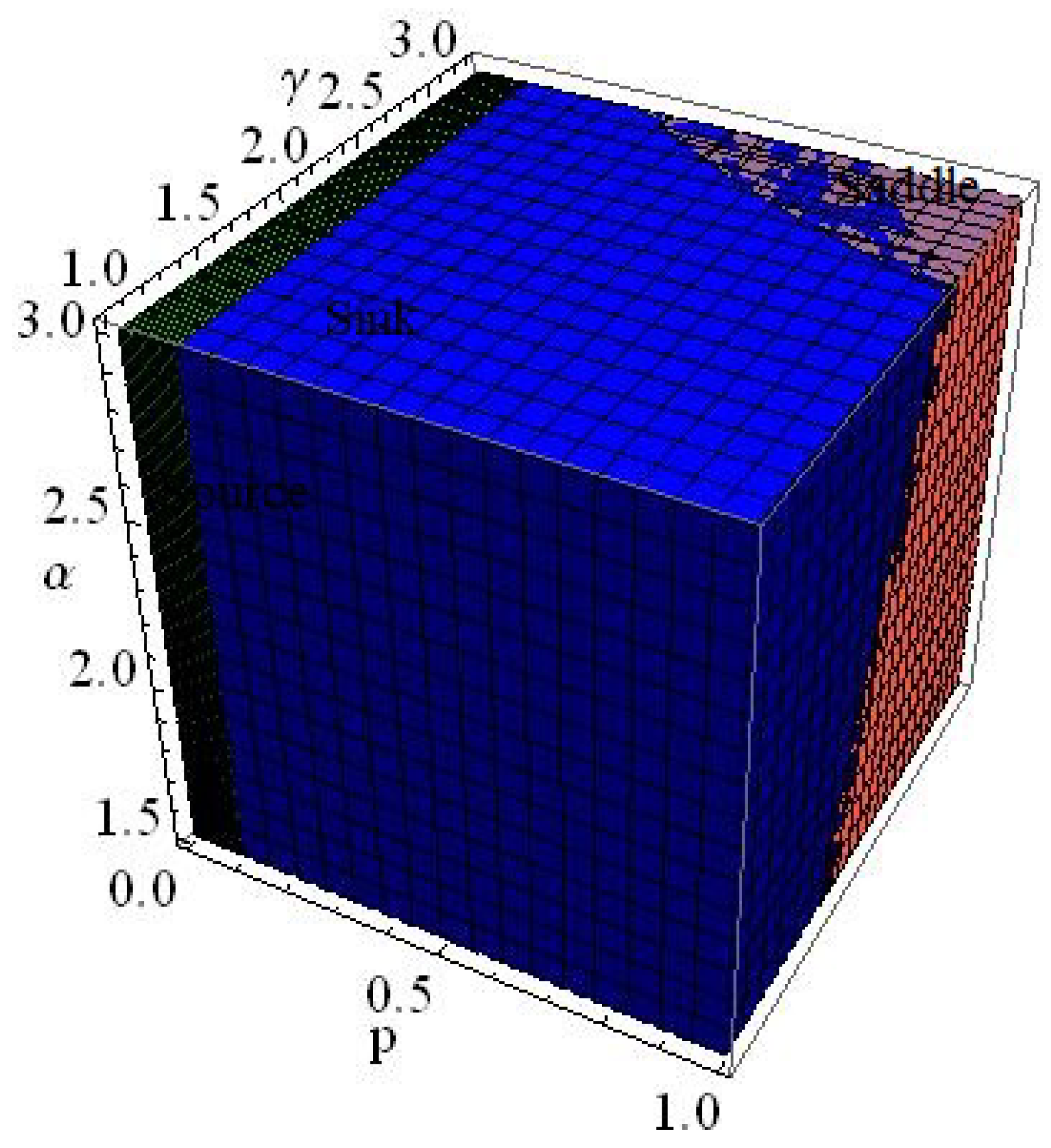
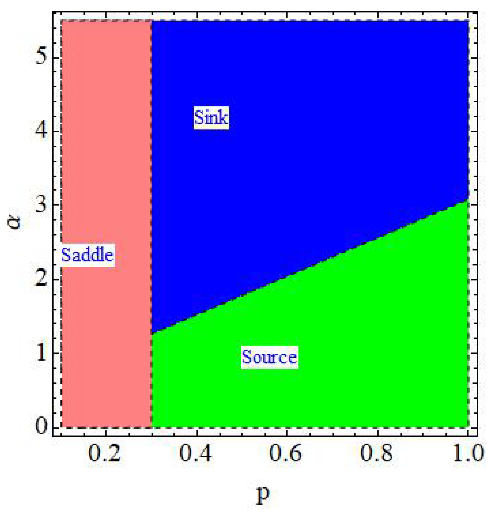
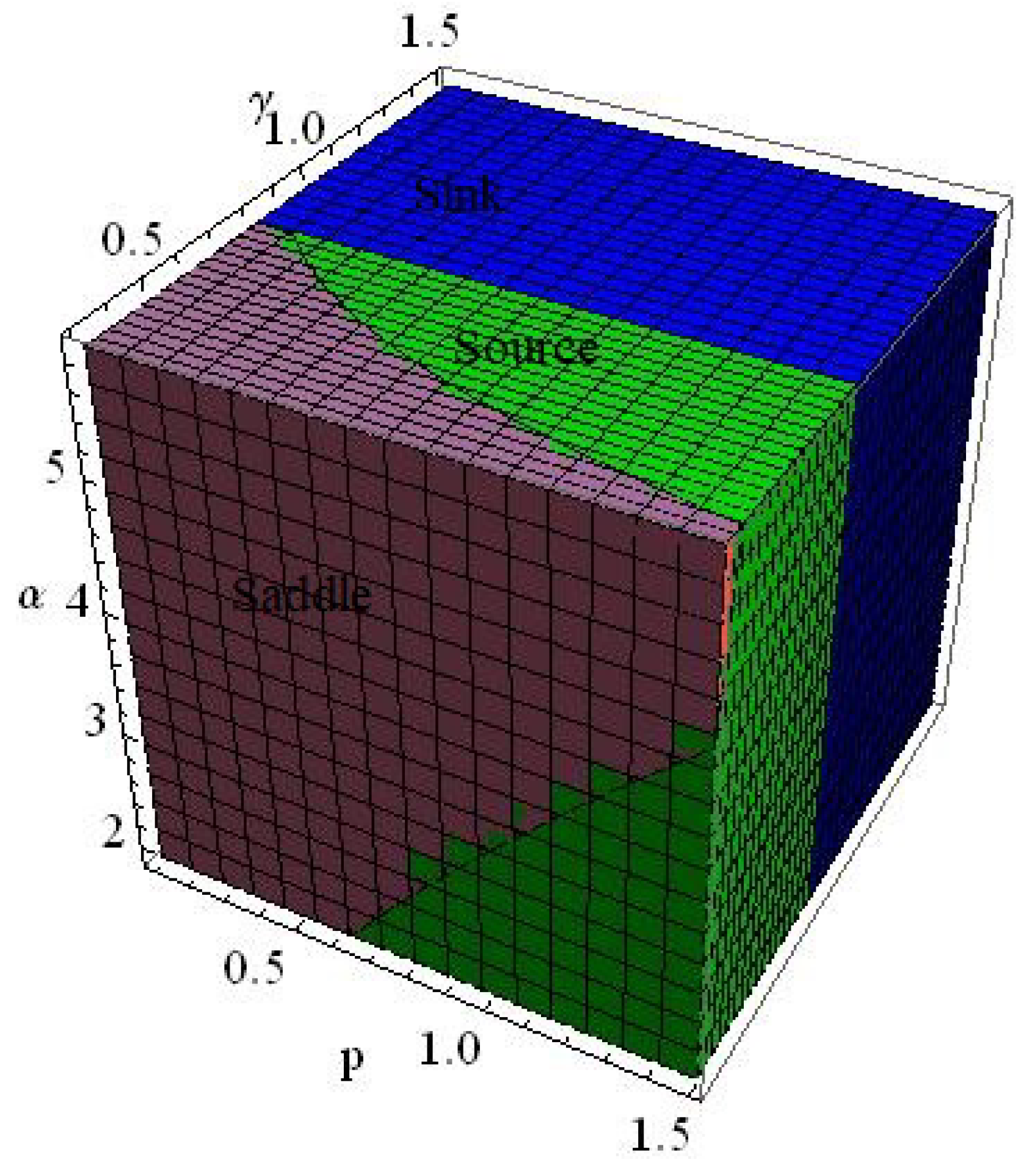
Theorem 1.

If

$$p<\gamma ,$$

(14)

and

$$p+\beta <1,$$

(15)

then every positive solution ${\left\{\left(S_t,I_t\right)\right\}}_{t=0}^{\infty }$ of the SI model (12) is bounded.

Proof. 

If ${\left\{\left(S_t,I_t\right)\right\}}_{t=0}^{\infty }$ is the positive solution of (12), then

$$\begin{array}{c}\hfill \left\{\begin{array}{c}\begin{array}{cc}\hfill S_{t+1}+I_{t+1}& =(1-p-\beta )(S_t+I_t)+(p-\gamma )I_t+N\beta ,\hfill \\ & \le (1-p-\beta )(S_t+I_t)+N\beta .\hfill \end{array}\hfill \end{array}\right.\end{array}$$

(16)

Furthermore, if $X_t=S_t+I_t$, then (16) becomes the following form:

$$\begin{array}{c}\hfill X_{t+1}\le (1-p-\beta )X_t+N\beta .\end{array}$$

(17)

From (17), one has

$$\begin{array}{c}\hfill W_{t+1}=(1-p-\beta )W_t+N\beta ,\end{array}$$

(18)

with solution

$$\begin{array}{c}\hfill W_t={\displaystyle \frac{N\beta (1-{(1-p-\beta )}^t)}{1-(1-p-\beta )}}+{(1-p-\beta )}^t{W}_0.\end{array}$$

(19)

Now, if (15) holds, then from (19), one gets

$$\begin{array}{c}\hfill {\displaystyle \underset{t\to \infty }{\lim }{W}_t=\frac{N\beta }{p+\beta }.}\end{array}$$

(20)

On further assuming that $X_0=S_0+I_0$, then from (17) and (20), the basic comparison test yields that $S_t+I_t\le {\displaystyle \frac{N\beta }{p+\beta }}$, and so, $0\le S_t\le {\displaystyle \frac{N\beta }{p+\beta }}$ and $0\le I_t\le {\displaystyle \frac{N\beta }{p+\beta }}$.  □

Theorem 2.

SI model (12) has a positive invariant set $\left[0,{\displaystyle \frac{\beta N}{p+\beta }}\right]\times \left[0,{\displaystyle \frac{\beta N}{p+\beta }}\right]$ , where $\forall t>0S_t+I_t\le {\displaystyle \frac{N\beta }{p+\beta }}$.

Proof. 

If ${\left\{\left(S_t,I_t\right)\right\}}_{t=0}^{\infty }$ is a positive solution of the SI model (12) with $S_0\times I_0\in \left[0,{\displaystyle \frac{\beta N}{p+\beta }}\right]\times \left[0,{\displaystyle \frac{\beta N}{p+\beta }}\right]$, then for $t=0$, one has $0\le S_1+I_1\le (1-p-\beta )(S_0+I_0)+N\beta \le {\displaystyle \frac{\beta N}{p+\beta }}$, and so, $0\le S_1\le {\displaystyle \frac{\beta N}{p+\beta }}$ and $0\le I_1\le {\displaystyle \frac{\beta N}{p+\beta }}$. Furthermore, easy simulation shows that $S_{m+1}\times I_{m+1}\in \left[0,{\displaystyle \frac{\beta N}{p+\beta }}\right]\times \left[0,{\displaystyle \frac{\beta N}{p+\beta }}\right]$ if $S_m\times I_m\in \left[0,{\displaystyle \frac{\beta N}{p+\beta }}\right]\times \left[0,{\displaystyle \frac{\beta N}{p+\beta }}\right]$.  □

3. Global Dynamics

We study the global dynamics for the SI model (12) at fixed points in this section. In order to proceed with this section, it is necessary first to examine the equilibria of the SI model (12). The straightforward calculation shows that $\forall p,N,\alpha ,\beta ,\gamma$, the SI model (12) has a disease-free fixed point (DFFP) ${\Omega }_1=\left({\displaystyle \frac{\beta N}{p+\beta }},0\right)$, and if $0<p<{\displaystyle \frac{\beta \left(\alpha -\beta -\gamma \right)}{\beta +\gamma }}$, then it has an epidemic fixed point (EFP) ${\Omega }_2=\left({\displaystyle \frac{\left(\beta +\gamma \right)N}{\alpha }},{\displaystyle \frac{\left(\alpha \beta -(\beta +\gamma )(p+\beta )\right)N}{\alpha (\beta +\gamma )}}\right)$. Additionally, variation matrix ${V|}_{\Omega }$ evaluated at $\Omega =(S,I)$ of the linearized system of the discrete model (12) under the map $\left(f_1,f_2\right)\mapsto \left(S_{t+1},I_{t+1}\right)$ is

$${V|}_{\Omega }≔\left(\begin{array}{cc}1-\beta -p-{\displaystyle \frac{\alpha }{N}}I& -{\displaystyle \frac{\alpha }{N}}S\\ {\displaystyle \frac{\alpha }{N}}I& 1-\beta -\gamma +{\displaystyle \frac{\alpha }{N}}S\end{array}\right),$$

(21)

where

$$\begin{array}{c}\hfill \left\{\begin{array}{c}{f}_1≔(1-p)S_t+\beta \left(N-S_t\right)-{\displaystyle \frac{\alpha }{N}}{S}_t{I}_t,\hfill \\ f_2≔{\displaystyle \frac{\alpha }{N}}{S}_t{I}_t+\left(1-\beta -\gamma \right)I_t.\hfill \end{array}\right.\end{array}$$

(22)

Hereafter, local as well as global dynamical analysis at ${\Omega }_{1,2}$ is given by existing theory [29,30,31]. At ${\Omega }_1$, (21), becomes

$${V|}_{{\Omega }_1}≔\left(\begin{array}{cc}1-p-\beta & -{\displaystyle \frac{\alpha \beta }{\beta +p}}\\ 0& {\displaystyle \frac{\alpha \beta }{\beta +p}}+1-\beta -\gamma \end{array}\right).$$

(23)

The characteristics equation of ${V|}_{{\Omega }_1}$ at ${\Omega }_1$ is

$${\lambda }^2-{\phi }_1\lambda +{\phi }_2=0,$$

(24)

where

$$\begin{array}{c}\hfill \begin{array}{c}\hfill \left\{\begin{array}{cc}{\phi }_1\hfill & =2-2\beta -\gamma -p+{\displaystyle \frac{\alpha \beta }{\beta +p}},\hfill \\ {\phi }_2\hfill & =1+{\displaystyle \frac{\alpha \beta }{p+\beta }}-\alpha \beta -\beta -\gamma +(p+\beta )\left(\beta +\gamma -1\right).\hfill \end{array}\right.\end{array}\end{array}$$

(25)

Now, local dynamics at ${\Omega }_1$ is studied by Theorems 1.3 and 1.6 of [29]. Before studying the local dynamics at ${\Omega }_{1,2}$ of the SI model (12), we first quote Theorems 1.3 and 1.6 of [29] for the convenience of our readers.

Theorem 3.

Consider the following equation:

$${\lambda }^2+{\phi }_1\lambda +{\phi }_2=0,$$

(26)

which is the characteristic equation of the linear system of a second-order difference equation: $x_{n+1}=f(x_n,x_{n-1}$ evaluated at the equilibrium point. Then, the following statements hold:

 (a) 

A necessary and sufficient condition for both roots of (26) to lie inside the open disc $\left|\lambda \right|<1$ is

$$|{\phi }_1|<1+{\phi }_2<2;$$

(27)

 (b) 

A necessary and sufficient condition for (26) to have one root with absolute value less than one and the other with absolute value greater than one is

$${\phi }_1^2-4{\phi }_2>0\mathrm{and}|{\phi }_1|>|1+{\phi }_2|;$$

(28)

 (c) 

A necessary and sufficient condition for both roots of (26) to have absolute value greater than one is

$$|{\phi }_1|>1\mathrm{and}|{\phi }_1|<|1+{\phi }_2|;$$

(29)

 (d) 

A necessary and sufficient condition for both roots of (26) to have absolute value equal to one is

$$|{\phi }_1|=|1+{\phi }_2|.$$

(30)

Theorem 4.

The sufficient condition for roots of (26) to lie inside the open disc is

$$|{\phi }_1|+|{\phi }_2|<1.$$

(31)

Theorem 5.

For local dynamics at ${\Omega }_1$, the following statements hold:

 (a) 

Necessary and sufficient (N & S) condition under which the roots of (24) lie inside the open unit disc is

$$\begin{array}{c}\hfill \begin{array}{ccc}& {\displaystyle \frac{(p+\beta )\left((p+\beta )(\beta +\gamma -1)-\beta -\gamma \right)}{\beta (p+\beta -1)}}<\alpha <\min \left\{{\displaystyle \frac{(p+\beta )\left(1+\beta +\gamma \right)+1}{\beta }},\right.\hfill & \\ & \left.{\displaystyle \frac{(p+\beta )\left(3\beta +2\gamma +p-(p+\beta )\left(\beta +\gamma -1\right)-4\right)}{\beta (2-p-\beta )}}\right\};\hfill \end{array}\end{array}$$

(32)

 (b) 

N & S condition under which the roots of (24) lie outside the open unit disc is

$$\begin{array}{c}\hfill \begin{array}{ccc}& {\displaystyle \frac{(p+\beta )\left((p+\beta )(\beta +\gamma -1)+\beta +\gamma +2\right)}{\beta (p+\beta -1)}}<\alpha <\min \left\{{\displaystyle \frac{(p+\beta )\left(1+\beta +\gamma \right)+1}{\beta }},\right.\hfill & \\ & \left.{\displaystyle \frac{(p+\beta )\left(3\beta +2\gamma +p-(p+\beta )\left(\beta +\gamma -1\right)-4\right)}{\beta (2-p-\beta )}}\right\};\hfill \end{array}\end{array}$$

(33)

 (c) 

N & S condition under which at least one root of (24) lies inside the open unit disc is

$$\begin{array}{c}\hfill \begin{array}{cc}& {\displaystyle \frac{(p+\beta )(\gamma -p)}{\beta }}<\alpha <{\displaystyle \frac{(p+\beta )\left(3\beta +2\gamma +p-(p+\beta )\left(\beta +\gamma -1\right)-4\right)}{\beta (2-p-\beta )}};\hfill \end{array}\end{array}$$

(34)

 (d) 

N & S condition under which the roots of (24) lie on othe pen unit disc is

$$\begin{array}{c}\hfill \begin{array}{c}\hfill \alpha ={\displaystyle \frac{(p+\beta )\left(3\beta +2\gamma +p-(p+\beta )\left(\beta +\gamma -1\right)-4\right)}{\beta (2-p-\beta )}}.\end{array}\end{array}$$

(35)

Proof. 

(a). In view of (27), one has $\left|{\phi }_1\right|=\left|2-2\beta -\gamma -p+{\displaystyle \frac{\alpha \beta }{\beta +p}}\right|<1+{\phi }_2=1+(1+{\displaystyle \frac{\alpha \beta }{p+\beta }}-\alpha \beta -\beta -\gamma +(p+\beta )\left(\beta +\gamma -1\right))<2$, which further gives the following set of inequalities:

$$\begin{array}{c}\hfill -2-{\displaystyle \frac{\alpha \beta }{p+\beta }}+\alpha \beta -(p+\beta )(\beta +\gamma -1)+\beta +\gamma <2-2\beta -p-\gamma +{\displaystyle \frac{\alpha \beta }{p+\beta }},\end{array}$$

(36)

$$\begin{array}{c}\hfill 2-2\beta -p-\gamma +{\displaystyle \frac{\alpha \beta }{p+\beta }}<3+{\displaystyle \frac{\alpha \beta }{p+\beta }}-\alpha \beta +(p+\beta )(\beta +\gamma -1)-\beta -\gamma ,\end{array}$$

(37)

and

$$\begin{array}{c}\hfill 2+{\displaystyle \frac{\alpha \beta }{p+\beta }}-\alpha \beta +(p+\beta )(\beta +\gamma -1)-\beta -\gamma <2.\end{array}$$

(38)

Furthermore, from (36), (37), and (38), one gets

$$\begin{array}{c}\hfill \alpha <{\displaystyle \frac{(p+\beta )\left(1+\beta +\gamma \right)+1}{\beta }},\end{array}$$

(39)

$$\begin{array}{c}\hfill \alpha <{\displaystyle \frac{(p+\beta )\left(3\beta +2\gamma +p-(p+\beta )\left(\beta +\gamma -1\right)-4\right)}{\beta (2-p-\beta )}},\end{array}$$

(40)

and

$$\begin{array}{c}\hfill \alpha >{\displaystyle \frac{(p+\beta )\left((p+\beta )(\beta +\gamma -1)-\beta -\gamma \right)}{\beta (p+\beta -1)}}.\end{array}$$

(41)

Finally, combining (39), (40) and (41), one obtains the desired computable N & S parametric condition (32) under which characteristic roots of (24) lie inside the open unit disc. Likewise, the straightforward calculation yields that N & S parametric condition under which the characteristic roots of the characteristics Equation (24) lies (b) outside, (c) at least one root lies inside, (d) on the open unit disc if ${\displaystyle \frac{(p+\beta )\left((p+\beta )(\beta +\gamma -1)+\beta +\gamma +2\right)}{\beta (p+\beta -1)}}$$<\alpha <\min \left\{{\displaystyle \frac{(p+\beta )\left(1+\beta +\gamma \right)+1}{\beta }},{\displaystyle \frac{(p+\beta )\left(3\beta +2\gamma +p-(p+\beta )\left(\beta +\gamma -1\right)-4\right)}{\beta (2-p-\beta )}}\right\}$, ${\displaystyle \frac{(p+\beta )(\gamma -p)}{\beta }}<\alpha <$${\displaystyle \frac{(p+\beta )\left(3\beta +2\gamma +p-(p+\beta )\left(\beta +\gamma -1\right)-4\right)}{\beta (2-p-\beta )}}$ and finally, $\alpha ={\displaystyle \frac{(p+\beta )\left(3\beta +2\gamma +p-(p+\beta )\left(\beta +\gamma -1\right)-4\right)}{\beta (2-p-\beta )}}$, respectively.  □

Remark 1.

It is noted here that ${\Omega }_1$ the SI model (12) is a sink, unstable (repeller), saddle, and nonhyperbolic if parametric conditions, which are depicted in (32), (33), (34) and (35), hold, respectively.

Theorem 6.

Sufficient condition under which the roots of (24) lie inside the open unit disc is

$$\begin{array}{c}\hfill \alpha >{\displaystyle \frac{(p+\beta )\left(3\beta +2\gamma +p-(p+\beta )\left(\beta +\gamma -1\right)-4\right)}{\beta (2-p-\beta )}}.\end{array}$$

(42)

Proof. 

In view of (31), one has $\left|{\phi }_1\right|+\left|{\phi }_2\right|=\left|2-2\beta -\gamma -p+{\displaystyle \frac{\alpha \beta }{\beta +p}}\right|+$$\left|1+{\displaystyle \frac{\alpha \beta }{p+\beta }}-\alpha \beta -\beta -\gamma +(p+\right.\left.\beta )\left(\beta +\gamma -1\right)\right|<1$, that is, $\alpha >{\displaystyle \frac{(p+\beta )\left(3\beta +2\gamma +p-(p+\beta )\left(\beta +\gamma -1\right)-4\right)}{\beta (2-p-\beta )}}$ is the desired computable condition under which the roots of (24) lie inside the open unit disc.  □

Remark 2.

If the condition (42) holds, then ${\Omega }_1$ of the SI model (12) is a sink.

Example 1.

If $\beta =0.9$ and $\gamma =1.5$, then at ${\Omega }_1$, the dynamics of the SI model (12) are given in Figure 1.

Example 2.

If $\beta =0.9$, then at ${\Omega }_1$, the dynamics of the SI model (12) are given in Figure 2.

Theorem 7.

If

$$\begin{array}{c}\hfill \alpha <{\displaystyle \frac{(\beta +\gamma )(p+\beta )}{\beta }},\end{array}$$

(43)

then ${\Omega }_1$ of the SI model (12) is a global attractor.

Proof. 

From the second equation of the SI model (12), one has

$$\begin{array}{c}\hfill \begin{array}{cc}\hfill I_{t+1}=& (1-\beta -\gamma )I_t+{\displaystyle \frac{\alpha }{N}}{S}_t{I}_t,\hfill \\ \hfill \le & (1-\beta -\gamma )I_t+{\displaystyle \frac{\alpha }{N}}\left({\displaystyle \frac{\beta N}{p+\beta }}\right)I_t,\hfill \\ \hfill =& (1-\beta -\gamma )I_t+{\displaystyle \frac{\alpha \beta }{p+\beta }}{I}_t,\hfill \\ \hfill =& \left(1-\beta -\gamma +{\displaystyle \frac{\alpha \beta }{p+\beta }}\right)I_t.\hfill \end{array}\end{array}$$

(44)

From (44), one consider the first-order homogeneous difference equation $y_{t+1}=\left(1-\beta -\gamma +{\displaystyle \frac{\alpha \beta }{p+\beta }}\right)y_t$ with the solution $y_t={\left(1-\beta -\gamma +{\displaystyle \frac{\alpha \beta }{p+\beta }}\right)}^t{n}_0$, where $n_0$ depends on $y_0$. Furthermore, if $1-\beta -\gamma +{\displaystyle \frac{\alpha \beta }{p+\beta }}<1$, that is, $\alpha <{\displaystyle \frac{(\beta +\gamma )(p+\beta )}{\beta }}$ then one can conclude that ${\left\{\left(y_t\right)\right\}}_{t=0}^{\infty }$ is bounded, and hence, ${\displaystyle \underset{t\to \infty }{\lim }{I}_t=0}$ by assuming that $y_0=I_0$. From this, one has for any $\epsilon >0\exists$ a natural number $m_0$ such that $I_t<\epsilon$$\forall t>m_0$. Therefore, from (12), we obtain that

$$\begin{array}{c}\hfill \left(1-{\displaystyle \frac{\alpha \epsilon }{N}}-p-\beta \right)S_t+N\beta \le S_{t+1}\le (1-p-\beta )S_t+N\beta .\end{array}$$

(45)

The left (respectively, right) inequality of (45) implies that for any ${\epsilon }_1>0\exists m_1>m_0$ (respectively, ${\epsilon }_2>0\exists m_2>m_0$) such that $S_t\ge {\displaystyle \frac{N\beta }{\frac{\alpha \epsilon }{N}+p+\beta }}-{\epsilon }_1\forall t>m_1$ (respectively, $S_t\le {\displaystyle \frac{N\beta }{p+\beta }}+{\epsilon }_2\forall t>m_2$). Now, if one assume $m_3=\max \left\{m_1,m_2\right\}$ then one obtain that ${\displaystyle \frac{N\beta }{\frac{\alpha \epsilon }{N}+p+\beta }}-{\epsilon }_1\le S_t\le {\displaystyle \frac{N\beta }{p+\beta }}+{\epsilon }_2\forall t\ge m_3$. But $\epsilon ,{\epsilon }_1$, and ${\epsilon }_2$ are arbitrary; so, finally, one gets ${\displaystyle \underset{t\to \infty }{\lim }{S}_t=\frac{N\beta }{p+\beta }}$.  □

Hereafter, the global dynamics at ${\Omega }_2$ of the SI model (12) are studied. At ${\Omega }_2$, (21) gives

$${V|}_{{\Omega }_2}≔\left(\begin{array}{cc}1-{\displaystyle \frac{\alpha \beta }{\beta +\gamma }}& -\beta -\gamma \\ {\displaystyle \frac{\alpha \beta }{\beta +\gamma }}-p-\beta & 1\end{array}\right),$$

(46)

with

$${\lambda }^2-{\phi }_1\lambda +{\phi }_2=0,$$

(47)

where

$$\begin{array}{c}\hfill \begin{array}{c}\hfill \left\{\begin{array}{cc}{\phi }_1\hfill & =2-{\displaystyle \frac{\alpha \beta }{\beta +\gamma }},\hfill \\ {\phi }_2\hfill & =1-{\displaystyle \frac{\alpha \beta }{\beta +\gamma }}+\alpha \beta -\left(p+\beta \right)(\beta +\gamma ).\hfill \end{array}\right.\end{array}\end{array}$$

(48)

Theorem 8.

For ${\Omega }_2$, the following statements hold:

 (a) 

N & S condition under which the roots of (47) lie inside the open unit disc is

$$\begin{array}{c}\hfill \begin{array}{cc}& \max \left\{{\displaystyle \frac{(p+\beta )(\beta +\gamma )}{\beta }},{\displaystyle \frac{(p+\beta ){(\beta +\gamma )}^2}{\beta (\gamma +\beta -1)}}\right\}<\alpha <{\displaystyle \frac{(\beta +\gamma )\left((p+\beta )(\beta +\gamma )-4\right)}{\beta (\gamma +\beta -2)}};\hfill \end{array}\end{array}$$

(49)

 (b) 

N & S condition under which the roots of (47) lie outside the open unit disc is

$$\begin{array}{c}\hfill \begin{array}{ccc}& {\displaystyle \frac{(p+\beta )(\beta +\gamma )}{\beta }}<\alpha <\min \left\{{\displaystyle \frac{(\beta +\gamma )\left((p+\beta )(\beta +\gamma )-4\right)}{\beta (\gamma +\beta -2)}},\right.\hfill & \\ & \left.{\displaystyle \frac{(\beta +\gamma )\left((p+\beta )(\beta +\gamma )-2\right)}{\beta (\gamma +\beta -1)}}\right\};\hfill \end{array}\end{array}$$

(50)

 (c) 

N & S condition under which at least one root of (47) lies inside the open unit disc is

$$\begin{array}{c}\hfill \begin{array}{ccc}& \max \left\{{\displaystyle \frac{2(\gamma +\beta )\left(\gamma +\beta +\sqrt{(\beta +\gamma )(\gamma -p)}\right)}{\beta }},\right.\hfill & \\ & \left.{\displaystyle \frac{2(\gamma +\beta )\left(\gamma +\beta -\sqrt{(\beta +\gamma )(\gamma -p)}\right)}{\beta }}\right\}<\alpha <{\displaystyle \frac{(\gamma +\beta )\left(\right(p+\beta \left)\right(\beta +\gamma )-4)}{\beta (\gamma +\beta -2)}};\hfill \end{array}\end{array}$$

(51)

 (d) 

N & S condition under which the roots of (47) lie on the open unit disc is

$$\begin{array}{c}\hfill \begin{array}{cc}& \alpha ={\displaystyle \frac{(p+\beta )(\beta +\gamma )}{\beta }},\hfill \end{array}\end{array}$$

(52)

or

$$\begin{array}{c}\hfill \begin{array}{c}\hfill \alpha ={\displaystyle \frac{(\gamma +\beta )\left((p+\beta )(\beta +\gamma )-4\right)}{\beta (\gamma +\beta -2)}}.\end{array}\end{array}$$

(53)

Proof. 

(a). If $\left|{\phi }_1\right|=\left|2-{\displaystyle \frac{\alpha \beta }{\beta +\gamma }}\right|<1+{\phi }_2=1+(1-{\displaystyle \frac{\alpha \beta }{\beta +\gamma }}+\alpha \beta -\left(p+\beta \right)(\beta +\gamma ))<2$, that is, $\max \left\{{\displaystyle \frac{(p+\beta )(\beta +\gamma )}{\beta }},{\displaystyle \frac{(p+\beta ){(\beta +\gamma )}^2}{\beta (\gamma +\beta -1)}}\right\}<\alpha <{\displaystyle \frac{(\beta +\gamma )\left(\right(p+\beta \left)\right(\beta +\gamma )-4)}{\beta (\gamma +\beta -2)}}$, then one gets the desired conclusion, indicating that the roots of (47) lie inside the open unit disc. In a similar way, one can easily achieve that the N & S parametric condition under which the roots of (47) lie (a) outside and (b) at least one root lies inside (c) on the open unit disc if ${\displaystyle \frac{(p+\beta )(\beta +\gamma )}{\beta }}<\alpha <\min \left\{{\displaystyle \frac{(\beta +\gamma )\left(\right(p+\beta \left)\right(\beta +\gamma )-4)}{\beta (\gamma +\beta -2)}},{\displaystyle \frac{(\beta +\gamma )\left(\right(p+\beta \left)\right(\beta +\gamma )-2)}{\beta (\gamma +\beta -1)}}\right\}$, $\max \left\{{\displaystyle \frac{2(\gamma +\beta )\left(\gamma +\beta +\sqrt{(\beta +\gamma )(\gamma -p)}\right)}{\beta }},{\displaystyle \frac{2(\gamma +\beta )\left(\gamma +\beta -\sqrt{(\beta +\gamma )(\gamma -p)}\right)}{\beta }}\right\}<\alpha <{\displaystyle \frac{(\gamma +\beta )\left((p+\beta )(\beta +\gamma )-4\right)}{\beta (\gamma +\beta -2)}}$ and $\alpha ={\displaystyle \frac{(\gamma +\beta )\left((p+\beta )(\beta +\gamma )-4\right)}{\beta (\gamma +\beta -2)}}$ or $\alpha ={\displaystyle \frac{(p+\beta )(\beta +\gamma )}{\beta }}$, respectively.  □

Theorem 9.

Sufficient condition under which the roots of (47) lie inside the open unit disc is

$$\begin{array}{c}\hfill \alpha <{\displaystyle \frac{(\gamma +\beta )\left((p+\beta )(\beta +\gamma )-4\right)}{\beta (\gamma +\beta -2)}}.\end{array}$$

(54)

Proof. 

The simple calculation $\left|{\phi }_1\right|+\left|{\phi }_2\right|=\left|2-{\displaystyle \frac{\alpha \beta }{\beta +\gamma }}\right|+|1+(1-{\displaystyle \frac{\alpha \beta }{\beta +\gamma }}+\alpha \beta -\left(p+\beta \right)(\beta +\gamma ))|<1$, that is, $\alpha <{\displaystyle \frac{(\gamma +\beta )\left((p+\beta )(\beta +\gamma )-4\right)}{\beta (\gamma +\beta -2)}}$ yields the desired conclusion.  □

Example 3.

If $\beta =0.187$ and $\gamma =0.299$ then at ${\Omega }_2$, dynamics of te SI model (12) is given in Figure 3.

Example 4.

If $\beta =0.187$, then at ${\Omega }_2$, the dynamics of the SI model (12) are given in Figure 4.

Theorem 10.

${\Omega }_2$ of the SI model (12) is a global attractor if

$$\begin{array}{c}\hfill \begin{array}{c}\hfill \max \left\{{\displaystyle \frac{{(\beta +\gamma )}^2}{\beta }},{\displaystyle \frac{(\beta +\gamma )(\beta +p)}{\beta }}\right\}<\alpha <\min \left\{{\displaystyle \frac{(\beta +\gamma )(2+\beta +\gamma )}{\beta }},{\displaystyle \frac{(\beta +p)(\beta +\gamma +2)}{\beta }}\right\}.\end{array}\end{array}$$

(55)

Proof. 

It is noted that the SI model (12) takes the following form:

$$\begin{array}{cc}\hfill S_{t+1}+I_{t+1}=& (1-p-\beta )(S_t+I_t)-(\gamma -p)I_t+N\beta .\end{array}$$

(56)

Furthermore, if

$${\mathrm{Y}}_t=S_t+I_t,$$

(57)

then, from SI models (12) and (56), one gets

$$\begin{array}{c}\hfill {\mathrm{Y}}_{t+1}=(1-p-\beta ){\mathrm{Y}}_t-(\gamma -p)I_t+N\beta ,I_{t+1}=(1-\beta -\gamma )I_t+{\displaystyle \frac{\alpha }{N}}({\mathrm{Y}}_t-I_t)I_t.\end{array}$$

(58)

The first equation of system (58) yields

$$\begin{array}{c}\hfill (1-\beta -\gamma ){\mathrm{Y}}_t+N\beta \le {\mathrm{Y}}_{t+1}\le (1-p-\beta ){\mathrm{Y}}_t+N\beta .\end{array}$$

(59)

Now, for any $\delta >0\exists r_0$ such that $\forall t>r_0$, from (59), one has

$$\begin{array}{c}\hfill {\displaystyle \frac{N\beta }{\gamma +\beta }}-\delta ={\mathrm{Y}}_1^l\le {\mathrm{Y}}_t\le {\displaystyle \frac{N\beta }{p+\beta }}+\delta ={\mathrm{Y}}_1^u.\end{array}$$

(60)

From the second equation of (58) and (60), one obtains

$$\begin{array}{c}\hfill (1-\beta -\gamma )I_t+{\displaystyle \frac{\alpha }{N}}({\mathrm{Y}}_1^l-I_t)I_t\le I_{t+1},\end{array}$$

(61)

and

$$\begin{array}{c}\hfill I_{t+1}\le (1-\beta -\gamma )I_t+{\displaystyle \frac{\alpha }{N}}({\mathrm{Y}}_1^u-I_t)I_t.\end{array}$$

(62)

From (61) and (62), one denotes

$$\begin{array}{c}\hfill z_{t+1}^l=(1-\beta -\gamma )z_t^l+{\displaystyle \frac{\alpha }{N}}\left({\mathrm{Y}}_1^l-z_t^l\right)z_t^l,z_{t+1}^u=(1-\beta -\gamma )z_t^u+{\displaystyle \frac{\alpha }{N}}\left({\mathrm{Y}}_1^u-z_t^u\right)z_t^u,\end{array}$$

(63)

with the following simplified from:

$$\begin{array}{c}\hfill z_{t+1}^l={\displaystyle \frac{\alpha z_t^l}{N}}\left({\displaystyle \frac{N(1-\beta -\gamma )+\alpha {\mathrm{Y}}_1^l}{\alpha }}-z_t^l\right),z_{t+1}^u={\displaystyle \frac{\alpha z_t^u}{N}}\left({\displaystyle \frac{N(1-\beta -\gamma )+\alpha {\mathrm{Y}}_1^u}{\alpha }}-z_t^u\right).\end{array}$$

(64)

Now, it is noted that (64) becomes the following logistic difference equations:

$$\begin{array}{c}\hfill y_{t+1}^l=r^l{y}_t^l(1-y_t^l),y_{t+1}^u=r^u{y}_t^u(1-y_t^u),\end{array}$$

(65)

by using the following change in variables:

$$\begin{array}{c}\hfill z_t^l={\displaystyle \frac{N(1-\beta -\gamma )+\alpha {\mathrm{Y}}_1^l}{\alpha }}{y}_t^l,z_t^u={\displaystyle \frac{N(1-\beta -\gamma )+\alpha {\mathrm{Y}}_1^u}{\alpha }}{y}_t^u,\end{array}$$

(66)

where $r^l={\displaystyle \frac{N(1-\beta -\gamma )+\alpha {\mathrm{Y}}_1^l}{N}}$ and $r^u={\displaystyle \frac{N(1-\beta -\gamma )+\alpha {\mathrm{Y}}_1^u}{N}}$. It is important here to recall that the unique positive fixed point $1-{\displaystyle \frac{1}{r}}$ of the discrete logistic difference equation $y_{t+1}=r{y}_t(1-y_t)$ is globally asymptotically stable if $1<r<3$ (see [28]). Therefore, it is easy to verify that the first (respectively, second) difference equation of the (65) has a unique positive equilibrium point $1-{\displaystyle \frac{1}{r^l}}$$\left(\mathrm{respectively},1-{\displaystyle \frac{1}{r^u}}\right)$ which is globally stable if $1<{\displaystyle \frac{N(1-\beta -\gamma )+\alpha {\mathrm{Y}}_1^l}{N}}<3$, that is, ${\displaystyle \frac{{(\beta +\gamma )}^2}{\beta }}<\alpha <{\displaystyle \frac{(\beta +\gamma )(2+\beta +\gamma )}{\beta }}$$\left(\mathrm{respectively},1<{\displaystyle \frac{N(1-\beta -\gamma )+\alpha {\mathrm{Y}}_1^u}{N}}<3,\mathrm{that}\mathrm{is},{\displaystyle \frac{(\beta +\gamma )(p+\beta )}{\beta }}<\alpha <{\displaystyle \frac{(\beta +p)(2+\beta +\gamma )}{\beta }}\right)$. Additionally, if ∃ a natural number $r_1>r_0$ such that $\forall t\ge r_1$, then from (61) and (62), one has

$$\begin{array}{c}\hfill I_1^l={\mathrm{Y}}_1^l-{\displaystyle \frac{N(\gamma +\beta )}{\alpha }}-\delta \le I_t\le {\mathrm{Y}}_1^u-{\displaystyle \frac{N(\gamma +\beta )}{\alpha }}+\delta =I_1^u.\end{array}$$

(67)

Now, if (14) holds, then from the first equation of (58), one has

$$\begin{array}{c}\hfill (1-\beta -p){\mathrm{Y}}_t-(\gamma -p)I_1^u+N\beta \le {\mathrm{Y}}_{t+1}\le (1-\beta -p){\mathrm{Y}}_t-(\gamma -p)I_1^l+N\beta ,\end{array}$$

(68)

where, from it, one gets

$$\begin{array}{c}\hfill {\mathrm{Y}}_2^l={\displaystyle \frac{N\beta -(\gamma -p)I_1^u}{p+\beta }}-\delta \le {\mathrm{Y}}_t\le {\displaystyle \frac{N\beta -(\gamma -p)I_1^l}{p+\beta }}+\delta ={\mathrm{Y}}_2^u,\end{array}$$

(69)

if $\exists r_2$ such that $\forall t\ge r_2$, and additionally, one has ${\mathrm{Y}}_1^l<{\mathrm{Y}}_2^l<{\mathrm{Y}}_2^u<{\mathrm{Y}}_1^u$. Now, in view of the second equation of (58) and (69), one gets

$$\begin{array}{c}\hfill (1-\beta -\gamma )I_t+{\displaystyle \frac{\alpha }{N}}({\mathrm{Y}}_2^l-I_t)I_t\le I_{t+1},I_{t+1}\le (1-\beta -\gamma )I_t+{\displaystyle \frac{\alpha }{N}}({\mathrm{Y}}_2^u-I_t)I_t.\end{array}$$

(70)

Now, if ∃ a natural number $r_3>r_2$ such that $\forall t\ge r_3$, then from (70), a simple calculation yields

$$\begin{array}{c}\hfill I_2^l={\mathrm{Y}}_2^l-{\displaystyle \frac{N(\gamma +\beta )}{\alpha }}-\delta \le I_t\le {\mathrm{Y}}_2^u-{\displaystyle \frac{N(\gamma +\beta )}{\alpha }}+\delta =I_2^u.\end{array}$$

(71)

Furthermore, (71) also gives

$$\begin{array}{c}\hfill I_2^l={\mathrm{Y}}_2^l-{\displaystyle \frac{N(\gamma +\beta )}{\alpha }}-\delta ={\displaystyle \frac{N\beta }{p+\beta }}-{\displaystyle \frac{N(\gamma +\beta )}{\alpha }}-{\displaystyle \frac{(\gamma -p)}{\beta +p}}{I}_1^u-2\delta ,\end{array}$$

(72)

and

$$\begin{array}{c}\hfill I_2^u={\mathrm{Y}}_2^u-{\displaystyle \frac{N(\gamma +\beta )}{\alpha }}+\delta ={\displaystyle \frac{N\beta }{p+\beta }}-{\displaystyle \frac{N(\gamma +\beta )}{\alpha }}-{\displaystyle \frac{(\gamma -p)}{\beta +p}}{I}_1^l+2\delta .\end{array}$$

(73)

So, by induction, if ∃ a natural number $r_{k+2}$ such that $I_k^l\le I_t\le I_k^u\forall t\ge r_{k+2}$, then from (72) and (73), one obtains the following system:

$$\begin{array}{c}\hfill \begin{array}{c}\hfill \left\{\begin{array}{cc}{I}_{k+1}^l=\hfill & {\displaystyle \frac{N\beta }{p+\beta }}-{\displaystyle \frac{N(\beta +\gamma )}{\alpha }}-{\displaystyle \frac{(\gamma -p)}{p+\beta }}{I}_k^u-2\delta ,\hfill \\ I_{k+1}^u=\hfill & {\displaystyle \frac{N\beta }{p+\beta }}-{\displaystyle \frac{N(\beta +\gamma )}{\alpha }}-{\displaystyle \frac{(\gamma -p)}{p+\beta }}{I}_k^l+2\delta ,\hfill \end{array}\right.\end{array}\end{array}$$

(74)

with equilibrium $\left(I_k^l,I_k^u\right)=\left({\displaystyle \frac{\left\{\begin{array}{c}N\left(\alpha \beta -(\beta +\gamma )(p+\beta )\right)\\ \hspace{1em}\left(\beta -\gamma +2p\right)-2\alpha \\ \hspace{1em}\hspace{1em}\hspace{1em}\left(p+\beta \right)\left(\beta +\gamma \right)\delta \end{array}\right\}}{\alpha (\beta +\gamma )\left(\beta -\gamma +2p\right)}},{\displaystyle \frac{\left\{\begin{array}{c}N\left(\alpha \beta -(\beta +\gamma )(p+\beta )\right)\\ \hspace{1em}\left(\beta -\gamma +2p\right)+2\alpha \\ \hspace{1em}\hspace{1em}\hspace{1em}\left(p+\beta \right)\left(\beta +\gamma \right)\delta \end{array}\right\}}{\alpha (\beta +\gamma )\left(\beta -\gamma +2p\right)}}\right)$ which is a sink if $p>{\displaystyle \frac{\gamma -\beta }{2}}$. Furthermore, one has ${\displaystyle \underset{t\to \infty }{\lim }{I}_t=\underset{\delta \to 0}{\lim }\frac{\left\{\begin{array}{c}N\left(\alpha \beta -(\beta +\gamma )(p+\beta )\right)\\ \hspace{1em}\left(\beta -\gamma +2p\right)-2\alpha \\ \hspace{1em}\hspace{1em}\hspace{1em}\left(p+\beta \right)\left(\beta +\gamma \right)\delta \end{array}\right\}}{\alpha (\beta +\gamma )\left(\beta -\gamma +2p\right)}=\underset{\delta \to 0}{\lim }\frac{\left\{\begin{array}{c}N\left(\alpha \beta -(\beta +\gamma )(p+\beta )\right)\\ \hspace{1em}\left(\beta -\gamma +2p\right)+2\alpha \\ \hspace{1em}\hspace{1em}\hspace{1em}\left(p+\beta \right)\left(\beta +\gamma \right)\delta \end{array}\right\}}{\alpha (\beta +\gamma )\left(\beta -\gamma +2p\right)}=\frac{N\left(\alpha \beta -(\beta +\gamma )(p+\beta )\right)}{\alpha (\beta +\gamma )}}$. Now, using (67) in (69), one gets

$$\begin{array}{c}\hfill {\mathrm{Y}}_2^l={\displaystyle \frac{N\beta }{p+\beta }}+{\displaystyle \frac{N(\beta +\gamma )(\gamma -p)}{\alpha (p+\beta )}}-{\displaystyle \frac{(\gamma -p)}{p+\beta }}{\mathrm{Y}}_1^u-{\displaystyle \frac{\left(\beta +\gamma \right)\delta }{p+\beta }},\end{array}$$

(75)

and

$$\begin{array}{c}\hfill {\mathrm{Y}}_2^u={\displaystyle \frac{N\beta }{p+\beta }}+{\displaystyle \frac{N(\beta +\gamma )(\gamma -p)}{\alpha (p+\beta )}}-{\displaystyle \frac{(\gamma -p)}{p+\beta }}{\mathrm{Y}}_1^l+{\displaystyle \frac{\left(\beta +\gamma \right)\delta }{p+\beta }}.\end{array}$$

(76)

Finally, by induction, if $\exists r_{k+1}$ such that ${\mathrm{Y}}_k^l\le {\mathrm{Y}}_t\le {\mathrm{Y}}_k^u\forall t\ge r_{k+1}$, then from (75) and (76), one has the following system:

$$\begin{array}{c}\hfill \begin{array}{c}\hfill \left\{\begin{array}{cc}{\mathrm{Y}}_{k+1}^l=\hfill & {\displaystyle \frac{N\beta }{p+\beta }}+{\displaystyle \frac{N(\beta +\gamma )(\gamma -p)}{\alpha (p+\beta )}}-{\displaystyle \frac{(\gamma -p)}{p+\beta }}{\mathrm{Y}}_k^u-{\displaystyle \frac{\left(\beta +\gamma \right)\delta }{p+\beta }},\hfill \\ {\mathrm{Y}}_{k+1}^u=\hfill & {\displaystyle \frac{N\beta }{p+\beta }}+{\displaystyle \frac{N(\gamma +\beta )(\gamma -p)}{\alpha (p+\beta )}}-{\displaystyle \frac{(\gamma -p)}{p+\beta }}{\mathrm{Y}}_k^l+{\displaystyle \frac{\left(\beta +\gamma \right)\delta }{p+\beta }},\hfill \end{array}\right.\end{array}\end{array}$$

(77)

with $\left({\mathrm{Y}}_k^l,{\mathrm{Y}}_k^u\right)=\left({\displaystyle \frac{\left\{\begin{array}{c}N\left(\alpha \beta +(\gamma -p)(\beta +\gamma )\right)\\ \hspace{1em}\left(\beta -\gamma +2p\right)-\alpha {\left(\beta +\gamma \right)}^2\delta \end{array}\right\}}{\alpha (\beta +\gamma )\left(\beta -\gamma +2p\right)}},{\displaystyle \frac{\left\{\begin{array}{c}N\left(\alpha \beta +(\gamma -p)(\beta +\gamma )\right)\\ \hspace{1em}\left(\beta -\gamma +2p\right)+\alpha {\left(\beta +\gamma \right)}^2\delta \end{array}\right\}}{\alpha (\beta +\gamma )\left(\beta -\gamma +2p\right)}}\right)$ where ${\displaystyle \underset{t\to \infty }{\lim }{\mathrm{Y}}_t=\underset{\delta \to 0}{\lim }\frac{\left\{\begin{array}{c}N\left(\alpha \beta +(\gamma -p)(\beta +\gamma )\right)\\ \hspace{1em}\left(\beta -\gamma +2p\right)-\alpha {\left(\beta +\gamma \right)}^2\delta \end{array}\right\}}{\alpha (\beta +\gamma )\left(\beta -\gamma +2p\right)}=\underset{\delta \to 0}{\lim }\frac{\left\{\begin{array}{c}N\left(\alpha \beta +(\gamma -p)(\beta +\gamma )\right)\\ \hspace{1em}\left(\beta -\gamma +2p\right)+\alpha {\left(\beta +\gamma \right)}^2\delta \end{array}\right\}}{\alpha (\beta +\gamma )\left(\beta -\gamma +2p\right)}}$$={\displaystyle \frac{N\left(\alpha \beta +(\gamma -p)(\beta +\gamma )\right)}{\alpha (\beta +\gamma )}}$. Finally, in view (57), one has ${\displaystyle \underset{t\to \infty }{\lim }{S}_t=\underset{t\to \infty }{\lim }\left({\mathrm{Y}}_t-I_t\right)=\frac{\left(\beta +\gamma \right)N}{\alpha }}$.  □

4. Identification of Codimension-Two Bifurcation Sets at Ω₂

For the identification of said bifurcation sets at ${\Omega }_2$, from (48), one has the following setting:

$$\begin{array}{c}\hfill {\phi }_1=2+G,{\phi }_2=1+G+H,\end{array}$$

(78)

where

$$\begin{array}{c}\hfill \begin{array}{c}\hfill \left\{\begin{array}{cc}G=\hfill & -{\displaystyle \frac{\alpha \beta }{\beta +\gamma }},\hfill \\ H=\hfill & \alpha \beta -(\beta +\gamma )(p+\beta ).\hfill \end{array}\right.\end{array}\end{array}$$

(79)

Additionally, roots of (47) are

$$\begin{array}{cc}\hfill {\lambda }_{1,2}& ={\displaystyle \frac{2+G\pm \sqrt{\Delta }}{2}},\end{array}$$

(80)

where

$$\begin{array}{c}\hfill \begin{array}{cc}\hfill \Delta =& {\left(G+2\right)}^2-4\left(H+G+1\right),\hfill \\ \hfill =& {\left(2-{\displaystyle \frac{\alpha \beta }{\beta +\gamma }}\right)}^2-4\left(1-{\displaystyle \frac{\alpha \beta }{\beta +\gamma }}+\alpha \beta -(\beta +\gamma )(p+\beta )\right).\hfill \end{array}\end{array}$$

(81)

From this, one can conclude the following:

(i)

If $H=4=-G$, then from (80), we obtain ${\lambda }_{1,2}=-1$ with $\alpha ={\displaystyle \frac{4(\beta +\gamma )}{\beta }}$ and $p={\displaystyle \frac{4(\beta +\gamma -1)}{\beta +\gamma }}-\beta$, and hence, at ${\Omega }_2$, the 1:2 strong resonance bifurcation set is

$$\begin{array}{cc}\hfill {\mathcal{F}}_{12}{|}_{{\Omega }_2}≔& \left\{\left(p,N,\alpha ,\beta ,\gamma \right):\alpha ={\displaystyle \frac{4(\beta +\gamma )}{\beta }},p={\displaystyle \frac{4(\beta +\gamma -1)}{\beta +\gamma }}-\beta \right\};\end{array}$$

(82)

(ii)

If $H=3=-G$, then from (80), we obtain ${\lambda }_{1,2}={\displaystyle \frac{-1\pm \sqrt{3}\iota }{2}}$ with $\alpha ={\displaystyle \frac{3(\beta +\gamma )}{\beta }}$ and $p={\displaystyle \frac{3(\beta +\gamma -1)}{\beta +\gamma }}-\beta$, and hence, at ${\Omega }_2$, the 1:3 strong resonance bifurcation set is

$$\begin{array}{cc}\hfill {\mathcal{F}}_{13}{|}_{{\Omega }_2}≔& \left\{\left(p,N,\alpha ,\beta ,\gamma \right):\alpha ={\displaystyle \frac{3(\beta +\gamma )}{\beta }},p={\displaystyle \frac{3(\beta +\gamma -1)}{\beta +\gamma }}-\beta \right\};\end{array}$$

(83)

(iii)

If $H=2=-G$ then from (80), we obtain ${\lambda }_{1,2}=\pm \iota$ with $\alpha ={\displaystyle \frac{2(\beta +\gamma )}{\beta }}$ and $p={\displaystyle \frac{2(\beta +\gamma -1)}{\beta +\gamma }}-\beta$, and hence, at ${\Omega }_2$, the 1:4 strong resonance bifurcation set is

$$\begin{array}{cc}\hfill {\mathcal{F}}_{14}{|}_{{\Omega }_2}≔& \left\{\left(p,N,\alpha ,\beta ,\gamma \right):\alpha ={\displaystyle \frac{2(\beta +\gamma )}{\beta }},p={\displaystyle \frac{2(\beta +\gamma -1)}{\beta +\gamma }}-\beta \right\}.\end{array}$$

(84)

Remark 3.

It is important to remark here that the $1:1$ resonance bifurcation does not exist at ${\Omega }_2$ of the SI model (12) if $H=0=G$ because G and H, which are depicted in (79), are never zero.

5. Codimension-Two Bifurcation at Ω₂

In this section, we study the codimension-two bifurcation by bifurcation theory [32,33,34,35,36,37].

5.1. 1:2 Strong Resonance Bifurcation Analysis

The detailed 1:2 strong resonance bifurcation analysis is given if (82) holds, where $\left(p,N,\alpha ,\beta ,\gamma \right)\in {\mathcal{F}}_{12}{|}_{{\Omega }_2}$, and furthermore, $\alpha$ and p are bifurcation parameters. To proceed, first, one needs to transform ${\Omega }_2$ to $\left(0,0\right)$ by

$$u_t=S_t-S^{\ast },v_t=I_t-I^{\ast },$$

(85)

where $S^{\ast }={\displaystyle \frac{(\beta +\gamma )N}{\alpha }}$ and $I^{\ast }={\displaystyle \frac{\left(\alpha \beta -(\beta +\gamma )(p+\beta )\right)N}{\alpha (\beta +\gamma )}}$. By utilizing (85) into (12), one obtains

$$\begin{array}{c}\hfill \begin{array}{c}\hfill \left\{\begin{array}{c}{u}_{t+1}=(1-p)(u_t+S^{\ast })+\beta (N-(u_t+S^{\ast }))-{\displaystyle \frac{\alpha }{N}}(u_t+S^{\ast })(v_t+I^{\ast })-S^{\ast },\hfill \\ v_{t+1}={\displaystyle \frac{\alpha }{N}}(u_t+S^{\ast })(v_t+I^{\ast })+(1-\beta -\gamma )(v_t+I^{\ast })-I^{\ast },\hfill \end{array}\right.\end{array}\end{array}$$

(86)

where, at $\left(0,0\right)$, the Taylor series expansion yields

$$\begin{array}{cc}\hfill \left(\begin{array}{c}{u}_{t+1}\\ v_{t+1}\end{array}\right)=& \left(\begin{array}{cc}1-p-\beta -{\displaystyle \frac{\alpha }{N}}{I}^{\ast }& -{\displaystyle \frac{\alpha }{N}}{S}^{\ast }\\ {\displaystyle \frac{\alpha }{N}}{I}^{\ast }& 1-\beta -\gamma +{\displaystyle \frac{\alpha }{N}}{S}^{\ast }\end{array}\right)\left(\begin{array}{c}{u}_t\\ v_t\end{array}\right)+\left(\begin{array}{c}-{\displaystyle \frac{\alpha }{N}}{u}_t{v}_t\\ \\ {\displaystyle \frac{\alpha }{N}}{u}_t{v}_t\end{array}\right).\hfill \end{array}$$

(87)

Furthermore, at ${\Omega }_2$, (87) takes the following form:

$$\begin{array}{cc}\hfill \left(\begin{array}{c}{u}_{t+1}\\ v_{t+1}\end{array}\right)=& \left(\begin{array}{cc}1-{\displaystyle \frac{\alpha \beta }{\beta +\gamma }}& -\beta -\gamma \\ {\displaystyle \frac{\alpha \beta }{\beta +\gamma }}-p-\beta & 1\end{array}\right)\left(\begin{array}{c}{u}_t\\ v_t\end{array}\right)+\left(\begin{array}{c}{f}_1(u_t,v_t)\\ f_2(u_t,v_t)\end{array}\right),\hfill \end{array}$$

(88)

where

$$\begin{array}{c}\hfill f_1(u_t,v_t)=-{\displaystyle \frac{\alpha }{N}}{u}_t{v}_t,f_2(u_t,v_t)={\displaystyle \frac{\alpha }{N}}{u}_t{v}_t.\end{array}$$

(89)

Now, from (88), if one defines

$$A\left(\varrho \right)=\left(\begin{array}{cc}1-{\displaystyle \frac{\alpha \beta }{\beta +\gamma }}& -\beta -\gamma \\ {\displaystyle \frac{\alpha \beta }{\beta +\gamma }}-p-\beta & 1\end{array}\right),$$

(90)

then

$$A_0=A\left({\varrho }_0\right){\mid }_{\varrho 0=\left(\alpha ,p\right)}=\left(\begin{array}{cc}-3& -\beta -\gamma \\ {\displaystyle \frac{4}{\beta +\gamma }}& 1\end{array}\right),$$

(91)

where $\varrho =\left(\alpha ,p\right)$ with ${\lambda }_{1,2}=-1$. Furthermore, corresponding to ${\lambda }_{1,2}=-1$, the straightforward calculation yields that $q_0=\left(\begin{array}{c}1\\ -{\displaystyle \frac{2}{\beta +\gamma }}\end{array}\right)$ and $q_1=\left(\begin{array}{c}1\\ -{\displaystyle \frac{3}{\beta +\gamma }}\end{array}\right)$ (respectively, $p_1=\left(\begin{array}{c}-2\\ -(\beta +\gamma )\end{array}\right)$ and $p_0=\left(\begin{array}{c}3\\ \beta +\gamma \end{array}\right)$) are eigenvector and generalized eigenvector of $A_0$ (respectively, $A_0^T$) satisfying $A_0{q}_0=-q_0$, $A_0^T{p}_0=p_1-p_0$, $\langle q_0,p_0\rangle =\langle q_1,p_1\rangle =1$, $A_0{q}_1=q_0-q_1$, $A_0^T{p}_1=-p_1$ and $\langle q_1,p_0\rangle =\langle q_0,p_1\rangle =0$, simultaneously. Now, if

$$\begin{array}{c}\hfill \left(\begin{array}{c}{u}_t\\ v_t\end{array}\right)≔n_t{q}_0+m_t{q}_1=\left(\begin{array}{cc}1& 1\\ -{\displaystyle \frac{2}{\beta +\gamma }}& -{\displaystyle \frac{3}{\beta +\gamma }}\end{array}\right)\left(\begin{array}{c}{n}_t\\ m_t\end{array}\right),\end{array}$$

(92)

with $x=\left(\begin{array}{c}{u}_t\\ v_t\end{array}\right)$, then one obtains

$$\begin{array}{c}\hfill \begin{array}{c}\hfill \left\{\begin{array}{c}{n}_t=\langle x,p_0\rangle =3u_t+(\beta +\gamma )v_t,\hfill \\ m_t=\langle x,p_1\rangle =-2u_t-(\beta +\gamma )v_t,\hfill \end{array}\right.\end{array}\end{array}$$

(93)

where, in $\left(n_t,m_t\right)$, (88) becomes

$$\begin{array}{c}\hfill \left(\begin{array}{c}{n}_{t+1}\\ m_{t+1}\end{array}\right)≔\left(\begin{array}{cc}-1+a\left(\varrho \right)& 1+b\left(\varrho \right)\\ c\left(\varrho \right)& -1+d\left(\varrho \right)\end{array}\right)\left(\begin{array}{c}{n}_t\\ m_t\end{array}\right)+\left(\begin{array}{c}{f}_3(n_t,m_t,\varrho )\\ f_4(n_t,m_t,\varrho )\end{array}\right),\end{array}$$

(94)

with

$$\begin{array}{c}\hfill \begin{array}{c}\hfill \left\{\begin{array}{c}{f}_3=\langle F\left(n_t{q}_0+m_t{q}_1,\varrho \right),p_0\rangle =a_{20}{n}_t^2+a_{11}{n}_t{m}_t+a_{02}{m}_t^2,\hfill \\ f_4=\langle F\left(n_t{q}_0+m_t{q}_1,\varrho \right),p_1\rangle =b_{20}{n}_t^2+b_{11}{n}_t{m}_t+b_{02}{m}_t^2,\hfill \end{array}\right.\end{array}\end{array}$$

(95)

and

$$F\left(x,\varrho \right)=\left(\begin{array}{c}-{\displaystyle \frac{4(\beta +\gamma )}{\beta N}}{u}_t{v}_t\\ {\displaystyle \frac{4(\beta +\gamma )}{\beta N}}{u}_t{v}_t\end{array}\right).$$

(96)

In view of (92), (95), and (96), one gets

$$\begin{array}{c}\hfill \begin{array}{c}\hfill \left\{\begin{array}{cc}{a}_{20}\hfill & =-{\displaystyle \frac{8(\beta +\gamma -3)}{\beta N}},a_{11}=-{\displaystyle \frac{20(\beta +\gamma -3)}{\beta N}},\hfill \\ a_{02}\hfill & =-{\displaystyle \frac{12(\beta +\gamma -3)}{\beta N}},b_{20}={\displaystyle \frac{8(\beta +\gamma -2)}{\beta N}},\hfill \\ b_{11}\hfill & ={\displaystyle \frac{20(\beta +\gamma -2)}{\beta N}},b_{02}={\displaystyle \frac{12(\beta +\gamma -2)}{\beta N}},\hfill \end{array}\right.\end{array}\end{array}$$

(97)

and

$$\begin{array}{c}\hfill \left\{\begin{array}{c}\begin{array}{cc}\hfill a\left(\varrho \right)=& \langle \left(A\left(\varrho \right)-A_0\right)q_0,p_0\rangle ={\displaystyle \frac{\alpha \beta (\beta +\gamma -3)}{\beta +\gamma }}-(\beta +\gamma )(\beta +p)+8,\hfill \\ \hfill b\left(\varrho \right)=& \langle \left(A\left(\varrho \right)-A_0\right)q_1,p_0\rangle ={\displaystyle \frac{\alpha \beta (\beta +\gamma -3)}{\beta +\gamma }}-(\beta +\gamma )(\beta +p)+8,\hfill \\ \hfill c\left(\varrho \right)=& \langle \left(A\left(\varrho \right)-A_0\right)q_0,p_1\rangle =\beta \left(\alpha \left({\displaystyle \frac{2}{\beta +\gamma }}-1\right)+\beta +\gamma \right)+p(\beta +\gamma )-4,\hfill \\ \hfill d\left(\varrho \right)=& \langle \left(A\left(\varrho \right)-A_0\right)q_1,p_1\rangle =\beta \left(\alpha \left({\displaystyle \frac{2}{\beta +\gamma }}-1\right)+\beta +\gamma \right)+p(\beta +\gamma )-4,\hfill \end{array}\hfill \end{array}\right.\end{array}$$

(98)

with $a\left({\varrho }_0\right)=b\left({\varrho }_0\right)=c\left({\varrho }_0\right)=d\left({\varrho }_0\right)=0$. Now, we define

$$B\left(\varrho \right)=\left(\begin{array}{cc}1+b\left(\varrho \right)& 0\\ -a\left(\varrho \right)& 1\end{array}\right),$$

(99)

with

$$\begin{array}{c}\hfill \left(\begin{array}{c}{n}_t\\ m_t\end{array}\right)≔B\left(\varrho \right)\left(\begin{array}{c}{p}_t\\ q_t\end{array}\right),\end{array}$$

(100)

which further becomes

$$\begin{array}{c}\hfill \left(\begin{array}{c}{p}_{t+1}\\ q_{t+1}\end{array}\right)≔\left(\begin{array}{cc}-1& 1\\ ϵ\left(\varrho \right)& -1+\sigma \left(\varrho \right)\end{array}\right)\left(\begin{array}{c}{p}_t\\ q_t\end{array}\right)+\left(\begin{array}{c}G\\ H\end{array}\right),\end{array}$$

(101)

where

$$\begin{array}{c}\hfill \left\{\begin{array}{c}ϵ\left(\varrho \right)=b\left(\varrho \right)c\left(\varrho \right)+c\left(\varrho \right)-a\left(\varrho \right)d\left(\varrho \right),\hfill \\ \sigma \left(\varrho \right)=d\left(\varrho \right)+a\left(\varrho \right),\hfill \end{array}\right.\end{array}$$

(102)

and

$$\begin{array}{c}\hfill \left(\begin{array}{c}G\\ H\end{array}\right)=B^{-1}\left(\varrho \right)\left(\begin{array}{c}{f}_3\left((1+b\left(\varrho \right))p_t,-a\left(\varrho \right)p_t+q_t,\varrho \right)\\ f_4\left((1+b\left(\varrho \right))p_t,-a\left(\varrho \right)p_t+q_t,\varrho \right)\end{array}\right).\end{array}$$

(103)

Now, if

$$\begin{array}{c}\hfill \varsigma =\left(\begin{array}{c}{\varsigma }_1\\ {\varsigma }_2\end{array}\right)=\left(\begin{array}{c}ϵ\left(\varrho \right)\\ \sigma \left(\varrho \right)\end{array}\right),\end{array}$$

(104)

then ${\varsigma }_1\left({\varrho }_0\right)={\varsigma }_2\left({\varrho }_0\right)=0$. Thus, (101), along with (102), (103) and (104), gives

$$\begin{array}{c}\hfill \left(\begin{array}{c}{p}_{t+1}\\ q_{t+1}\end{array}\right)=\left(\begin{array}{cc}-1& 1\\ {\varsigma }_1& -1+{\varsigma }_2\end{array}\right)\left(\begin{array}{c}{p}_t\\ q_t\end{array}\right)+\left(\begin{array}{c}G\left(p_t,q_t,\varrho \right)\\ H\left(p_t,q_t,\varrho \right)\end{array}\right),\end{array}$$

(105)

where

$$\begin{array}{c}\hfill \left\{\begin{array}{c}\begin{array}{cc}\hfill G\left(p_t,q_t,\varrho \right)=& g_{20}{p}_t^2+g_{11}{p}_t{q}_t+g_{02}{q}_t^2,\hfill \\ \hfill H\left(p_t,q_t,\varrho \right)=& h_{20}{p}_t^2+h_{11}{p}_t{q}_t+h_{02}{q}_t^2,\hfill \end{array}\hfill \end{array}\right.\end{array}$$

(106)

and

$$\begin{array}{c}\hfill \begin{array}{c}\hfill \left\{\begin{array}{cc}{g}_{20}=\hfill & a_{20}(1+b\left(\varrho \right))-a_{11}a\left(\varrho \right)+{\displaystyle \frac{a^2\left(\varrho \right)a_{02}}{1+b\left(\varrho \right)}},g_{11}=a_{11}-{\displaystyle \frac{2a\left(\varrho \right)a_{02}}{1+b\left(\varrho \right)}},g_{02}={\displaystyle \frac{a_{02}}{1+b\left(\varrho \right)}},\hfill \\ h_{20}=\hfill & {(1+b\left(\varrho \right))}^2{b}_{20}+(a_{20}-b_{11})(1+b\left(\varrho \right))a\left(\varrho \right)+(b_{02}-a_{11})a^2\left(\varrho \right)+{\displaystyle \frac{a^3\left(\varrho \right)a_{02}}{1+b\left(\varrho \right)}},\hfill \\ h_{11}=\hfill & a_{11}a\left(\varrho \right)-{\displaystyle \frac{2a^2\left(\varrho \right)a_{02}}{1+b\left(\varrho \right)}}-2a\left(\varrho \right)b_{02}+b_{11}(1+b\left(\varrho \right)),h_{02}=b_{02}+{\displaystyle \frac{a\left(\varrho \right)a_{02}}{1+b\left(\varrho \right)}},\hfill \end{array}\right.\end{array}\end{array}$$

(107)

$g_{jk}=h_{jk}=0\forall j,k>0$ and $j+k=3$. On utiliing

$$\begin{array}{c}\hfill \begin{array}{c}\hfill \left\{\begin{array}{c}{\displaystyle p_t=n_t+\sum _{2\le j+k\le 3}{\Phi }_{jk}\left(\varsigma \right)n_t^j,}\hfill \\ {\displaystyle q_t=m_t+\sum _{2\le j+k\le 3}{\Psi }_{jk}\left(\varsigma \right)n_t^j{m}_t^k,}\hfill \end{array}\right.\end{array}\end{array}$$

(108)

with

$$\begin{array}{c}\hfill \begin{array}{c}\hfill \left\{\begin{array}{cc}{\Phi }_{03}=\hfill & {\Psi }_{03}=0,{\Phi }_{20}={\displaystyle \frac{1}{2}}{g}_{20}+{\displaystyle \frac{1}{4}}{h}_{20},\hfill \\ {\Phi }_{11}=\hfill & {\displaystyle \frac{1}{2}}{g}_{20}+{\displaystyle \frac{1}{2}}{g}_{11}+{\displaystyle \frac{1}{2}}{h}_{20}+{\displaystyle \frac{1}{4}}{h}_{11},\hfill \\ {\Phi }_{02}=\hfill & {\displaystyle \frac{1}{2}}{g}_{11}+{\displaystyle \frac{1}{2}}{g}_{02}+{\displaystyle \frac{1}{8}}{h}_{20}+{\displaystyle \frac{1}{4}}{h}_{11}+{\displaystyle \frac{1}{4}}{h}_{02},{\Psi }_{20}={\displaystyle \frac{1}{2}}{h}_{20},\hfill \\ {\Psi }_{11}=\hfill & {\displaystyle \frac{1}{2}}{h}_{20}+{\displaystyle \frac{1}{2}}{h}_{11},{\Psi }_{02}={\displaystyle \frac{1}{4}}{h}_{11}+{\displaystyle \frac{1}{2}}{h}_{02},\hfill \\ {\Phi }_{30}=\hfill & {\Phi }_{21}={\Phi }_{12}={\Psi }_{30}={\Psi }_{21}={\Psi }_{12}=0,\hfill \end{array}\right.\end{array}\end{array}$$

(109)

one has the following 1:2 resonance normal form:

$$\begin{array}{c}\hfill \left(\begin{array}{c}{n}_{t+1}\\ m_{t+1}\end{array}\right)≔\left(\begin{array}{cc}-1& 1\\ {\varsigma }_1& -1+{\varsigma }_2\end{array}\right)\left(\begin{array}{c}{n}_t\\ m_t\end{array}\right)+\left(\begin{array}{c}0\\ C\left(\varsigma \right)n_t^3+D\left(\varsigma \right)n_t^2{m}_t\end{array}\right),\end{array}$$

(110)

where

$$\begin{array}{c}\hfill \begin{array}{c}\hfill \left\{\begin{array}{cc}C\left({\varsigma }_1\left({\varrho }_0\right),{\varsigma }_2\left({\varrho }_0\right)\right)=\hfill & {\displaystyle \frac{16\left(3{\beta }^2+\beta (6\gamma -8)+3{\gamma }^2-8\gamma +4\right)}{{\beta }^2{N}^2}},\hfill \\ D\left({\varsigma }_1\left({\varrho }_0\right),{\varsigma }_2\left({\varrho }_0\right)\right)=\hfill & {\displaystyle \frac{16\left(7{\beta }^2+2\beta (7\gamma -6)+\gamma (7\gamma -12)+8\right)}{{\beta }^2{N}^2}}.\hfill \end{array}\right.\end{array}\end{array}$$

(111)

Finally, this theoretical analysis gives the following result.

Theorem 11.

From (111), if $C\ne 0$ and $D+3C={\displaystyle \frac{64(\beta +\gamma -1)(4\beta +4\gamma -5)}{{\beta }^2{N}^2}}\ne 0$, then 1:2 strong resonance bifurcation exists at ${\Omega }_2$. Moreover, if $C>0$ (respectively, $C<0$), then ${\Omega }_2$ is elliptic (respectively, saddle), and finally, near 1:2 point, $3C+D\ne 0$ defines the bifurcation curves:

 (i) 

Pitchfork bifurcation curve:

$$\begin{array}{c}\hfill \begin{array}{cc}\hfill {\mathcal{F}}_{15}{|}_{{\Omega }_2}≔& \left\{\left({\varsigma }_1,{\varsigma }_2\right):{\varsigma }_1=0\right\},\hfill \end{array}\end{array}$$

(112)

and additionally, for ${\varsigma }_1<0$ there exists a nontrivial fixed point;

 (ii) 

Homologous bifurcation curve:

$$\begin{array}{c}\hfill \begin{array}{cc}\hfill {\mathcal{F}}_{16}{|}_{{\Omega }_2}≔& \left\{\left({\varsigma }_1,{\varsigma }_2\right):{\varsigma }_1=-{\displaystyle \frac{4}{5}}{\varsigma }_2+O\left({\left(|{\varsigma }_1|+|{\varsigma }_2|\right)}^2\right),{\varsigma }_1<0\right\};\hfill \end{array}\end{array}$$

(113)

 (iii) 

Nondegenerate N-S bifurcation curve:

$$\begin{array}{c}\hfill \begin{array}{cc}\hfill {\mathcal{F}}_{17}{|}_{{\Omega }_2}≔& \left\{\left({\varsigma }_1,{\varsigma }_2\right):{\varsigma }_1=-{\varsigma }_2+O\left({\left(|{\varsigma }_1|+|{\varsigma }_2|\right)}^2\right),{\varsigma }_1<0\right\};\hfill \end{array}\end{array}$$

(114)

 (iv) 

Heteroclinic bifurcation curve:

$$\begin{array}{c}\hfill \begin{array}{cc}\hfill {\mathcal{F}}_{18}{|}_{{\Omega }_2}≔& \left\{\left({\varsigma }_1,{\varsigma }_2\right):{\varsigma }_1=-{\displaystyle \frac{5}{3}}{\varsigma }_2+O\left({\left(|{\varsigma }_1|+|{\varsigma }_2|\right)}^2\right),{\varsigma }_1<0\right\}.\hfill \end{array}\end{array}$$

(115)

5.2. 1:3 Strong Resonance Bifurcation Analysis

If (83) holds, then from (46), one gets

$${V|}_{{\Omega }_2}=A_0=A\left({\varrho }_0\right){\mid }_{\varrho 0=\left(\alpha ,p\right)}=\left(\begin{array}{cc}-2& -\beta -\gamma \\ {\displaystyle \frac{3}{\beta +\gamma }}& 1\end{array}\right),$$

(116)

with ${\lambda }_{1,2}={\displaystyle \frac{-1\pm \sqrt{3}\iota }{2}}$ where $q=\left(\begin{array}{c}\beta +\gamma \\ {\displaystyle \frac{-3-\sqrt{3}\iota }{2}}\end{array}\right)$ and $p=\left(\begin{array}{c}{\displaystyle \frac{1-\sqrt{3}\iota }{2(\beta +\gamma )}}\\ -{\displaystyle \frac{\sqrt{3}\iota }{3}}\end{array}\right)$ are the corresponding eigenvector and adjoint eigenvector of $A_0$ satisfying $\langle p,q\rangle =1$, $A_0^{T}p={\displaystyle \frac{-1-\sqrt{3}\iota }{2}}p$, $A_{0}q={\displaystyle \frac{-1+\sqrt{3}\iota }{2}}q$, $A_0\overline{q}={\displaystyle \frac{-1-\sqrt{3}\iota }{2}}\overline{q}$ and $A_0^T\overline{p}={\displaystyle \frac{-1+\sqrt{3}\iota }{2}}\overline{q}$. Furthermore, if $Z=\left(\begin{array}{c}{u}_t\\ v_t\end{array}\right)\in {\mathbb{R}}^2$, where $Z_t=z_{t}q+{\overline{z}}_t\overline{q}$, then (88) gives

$$z_{t+1}={\displaystyle \frac{-1+\sqrt{3}\iota }{2}}{z}_t+g(z_t,{\overline{z}}_t,{\varrho }_0),$$

(117)

with

$$\begin{array}{c}\hfill \begin{array}{c}\hfill {\displaystyle g(z_t,{\overline{z}}_t,{\varrho }_0)=\langle p\left(\varrho \right),F\left(z_{t}q+{\overline{z}}_t\overline{q}\right)\rangle =\sum _{2\le j+k\le 3}\frac{g_{jk}}{j!k!}{z}_t^j{\overline{z}}_t^k,}\end{array}\end{array}$$

(118)

$$F\left(z_{t}q+{\overline{z}}_t\overline{q},\varrho \right)=\left(\begin{array}{c}-{\displaystyle \frac{3(\beta +\gamma )}{\beta N}}{u}_t{v}_t\\ \\ {\displaystyle \frac{3(\beta +\gamma )}{\beta N}}{u}_t{v}_t\end{array}\right),$$

(119)

and

$$\begin{array}{c}\hfill \begin{array}{c}\hfill \left\{\begin{array}{cc}{g}_{20}=\hfill & -{\displaystyle \frac{3(\beta +\gamma )}{2N\beta }}\left((\beta +\gamma )+\iota (2+\beta +\gamma )\sqrt{3}\right),\hfill \\ g_{11}=\hfill & {\displaystyle \frac{3(\beta +\gamma )}{2N\beta }}\left(3+\iota (\beta +\gamma -3)\sqrt{3})\right),\hfill \\ g_{02}=\hfill & {\displaystyle \frac{3(\beta +\gamma )}{4N\beta }}\left(2(3+\beta +\gamma )+\iota (3+\sqrt{3}+2(\beta +\gamma ))\right).\hfill \end{array}\right.\end{array}\end{array}$$

(120)

Now, to eliminate quadratic terms from (117), one uses the following transformation:

$$\begin{array}{c}\hfill z_t=w_t+{\displaystyle \frac{1}{2}}{h}_{20}{w}_t^2+h_{11}{w}_t\overline{w_t}+{\displaystyle \frac{1}{2}}{h}_{20}{\overline{w_t}}^2,\end{array}$$

(121)

where it becomes

$$\begin{array}{c}\hfill {\displaystyle w_{t+1}={\lambda }_1{w}_t+\sum _{2\le j+k\le 3}\frac{{\sigma }_{jk}}{j!k!}{w}_t^j{\overline{w}}_t^k,}\end{array}$$

(122)

with

$$\begin{array}{c}\hfill \begin{array}{c}\hfill \left\{\begin{array}{cc}{\sigma }_{20}=\hfill & {\lambda }_1{h}_{20}+g_{20}-{\lambda }_1^2{h}_{20},{\sigma }_{11}={\lambda }_1{h}_{11}+g_{11}-{\left|{\lambda }_1\right|}^2{h}_{11},\hfill \\ {\sigma }_{30}=\hfill & 3(1-{\lambda }_1)g_{20}{h}_{20}+3g_{11}{\overline{h}}_{02}+3({\lambda }_1^3-{\lambda }_1^2)h_{20}^2+3({\lambda }_1^3-|{\lambda }_1{|}^2)h_{11}{\overline{h}}_{02}-3{\lambda }_1{\overline{g}}_{02}{h}_{11},\hfill \\ {\sigma }_{02}=\hfill & {\lambda }_1{h}_{02}+g_{02}-{\overline{{\lambda }_1}}^2{h}_{02},\hfill \\ {\sigma }_{21}=\hfill & \left\{\begin{array}{cc}& 2g_{11}{\overline{h}}_{11}+g_{11}{h}_{20}+2g_{20}{h}_{11}+g_{02}{\overline{h}}_{02}+2{\lambda }_1^2(\overline{{\lambda }_1}-1)h_{20}{h}_{11}-2{\lambda }_1{g}_{11}{h}_{20}\hfill \\ & -\overline{{\lambda }_1}{g}_{20}{h}_{11}+2|{\lambda }_1{|}^2({\lambda }_1-1){\left|h_{11}\right|}^2-2{\lambda }_1{h}_{11}{\overline{g}}_{11}\hfill \\ & +|{\lambda }_1{|}^2({\lambda }_1-1)h_{11}{h}_{20}-\overline{{\lambda }_1}{g}_{02}{h}_{02}+\overline{{\lambda }_1}({\lambda }_1^2-\overline{{\lambda }_1}){\left|h_{02}\right|}^2\hfill \end{array}\right\},\hfill \\ {\sigma }_{12}=\hfill & \left\{\begin{array}{cc}& 2g_{11}{h}_{11}+g_{11}{\overline{h}}_{20}+2g_{02}{\overline{h}}_{11}+g_{20}{h}_{02}\hfill \\ & +{\lambda }_1({\overline{{\lambda }_1}}^2-{\lambda }_1)h_{20}{h}_{02}-{\lambda }_1{\overline{g}}_{20}{h}_{11}\hfill \\ & -2{\lambda }_1{g}_{02}{h}_{20}-2\overline{{\lambda }_1}{g}_{11}{h}_{11}+2{\left|{\lambda }_1\right|}^2(\overline{{\lambda }_1}-1)h_{11}^2\hfill \\ & +|{\lambda }_1{|}^2(\overline{{\lambda }_1}-1)h_{11}{\overline{h}}_{20}+2{\overline{{\lambda }_1}}^2({\lambda }_1-1)h_{02}{\overline{h}}_{11}\hfill \\ & -2\overline{{\lambda }_1}{\overline{g}}_{11}{h}_{02}\hfill \end{array}\right\},\hfill \\ {\sigma }_{03}=\hfill & \left\{\begin{array}{cc}& 3g_{11}{h}_{02}+3g_{02}{\overline{h}}_{20}+3({\overline{{\lambda }_1}}^3-|{\lambda }_1{|}^2)h_{11}{h}_{02}\hfill \\ & -3\overline{{\lambda }_1}{g}_{02}{h}_{11}-3\overline{{\lambda }_1}{\overline{g}}_{20}{h}_{02}+3{\overline{{\lambda }_1}}^2(\overline{{\lambda }_1}-1)h_{02}{\overline{h}}_{20}\hfill \end{array}\right\}.\hfill \end{array}\right.\end{array}\end{array}$$

(123)

Now, it is noted that if

$$\begin{array}{cc}\hfill h_{20}={\displaystyle \frac{\sqrt{3}\iota }{3}}{g}_{20},h_{11}=& {\displaystyle \frac{3+\sqrt{3}\iota }{6}}{g}_{11},h_{02}=0,\end{array}$$

(124)

then the quadratic terms of (122) vanish, and furthermore, the cubic terms should vanish by the following transformation:

$$\begin{array}{c}\hfill w_{t+1}={\xi }_t+{\displaystyle \frac{1}{6}}{h}_{30}{\xi }_t^3+{\displaystyle \frac{1}{2}}{h}_{12}{\xi }_t{\overline{\xi }}_t^2+{\displaystyle \frac{1}{2}}{h}_{21}{\xi }_t^2{\overline{\xi }}_t+{\displaystyle \frac{1}{6}}{h}_{03}{\overline{\xi }}_t^3.\end{array}$$

(125)

From (125) and (122), we obtain

$$\begin{array}{c}\hfill {\displaystyle {\xi }_{t+1}=\frac{\sqrt{3}\iota -1}{2}{\xi }_t+\frac{1}{2}{g}_{02}{\overline{\xi }}_t^2+\sum _{2\le j+k\le 3}\frac{r_{jk}}{j!k!}{\xi }_t^j{\overline{\xi }}_t^k,}\end{array}$$

(126)

where

$$\begin{array}{c}\hfill \begin{array}{c}\hfill \left\{\begin{array}{cc}{r}_{30}=\hfill & {\displaystyle \frac{\sqrt{3}\iota -3}{2}}{h}_{30}+{\sigma }_{30},r_{21}={\sigma }_{21},\hfill \\ r_{12}=\hfill & \sqrt{3}\iota h_{12}+{\sigma }_{12},r_{03}={\displaystyle \frac{\sqrt{3}\iota -3}{2}}{h}_{03}+{\sigma }_{03}.\hfill \end{array}\right.\end{array}\end{array}$$

(127)

Now, further, it is noted from (127) that all quantities except $r_{21}$ vanish if

$$\begin{array}{c}\hfill \begin{array}{c}\hfill \left\{\begin{array}{cc}{h}_{30}=\hfill & {\displaystyle \frac{3+\sqrt{3}\iota }{6}}{\sigma }_{30},h_{12}={\displaystyle \frac{\sqrt{3}\iota }{3}}{\sigma }_{12},\hfill \\ h_{03}=\hfill & {\displaystyle \frac{3+\sqrt{3}\iota }{6}}{\sigma }_{03},h_{21}=0.\hfill \end{array}\right.\end{array}\end{array}$$

(128)

Hence, the 1:3 resonance normal form is

$$\begin{array}{c}\hfill {\xi }_{t+1}={\displaystyle \frac{\sqrt{3}\iota -1}{2}}{\xi }_t+C(\alpha ,p){\overline{\xi }}_t^2+D(\alpha ,p){\xi }_t{\left|{\xi }_t\right|}^2,\end{array}$$

(129)

where

$$\begin{array}{c}\hfill \begin{array}{c}\hfill \left\{\begin{array}{cc}C(\alpha ,p)=\hfill & {\displaystyle \frac{3(\beta +\gamma )}{8\beta N}}\left((6+2(\beta +\gamma ))+\iota \left(2(\beta +\gamma )+3+\sqrt{3}\right)\right),\hfill \\ D(\alpha ,p)=\hfill & {\displaystyle \frac{9{(\beta +\gamma )}^2}{8{\beta }^2{N}^2}}(\left(7{(\beta +\gamma )}^2-24(\beta +\gamma )+24+\right.\hfill \\ & \left.\iota \left(\sqrt{3}{(\beta +\gamma )}^2-8\sqrt{3}(\beta +\gamma )\right)\right).\hfill \end{array}\right.\end{array}\end{array}$$

(130)

Finally, if

$$\begin{array}{c}\hfill \left\{\begin{array}{c}\begin{array}{cc}\hfill C_1(\alpha ,p)=& 3{\overline{\lambda }}_{1}C(\alpha ,p),\hfill \\ \hfill =& -{\displaystyle \frac{9(\beta +\gamma )}{16\beta N}}\left(2(1-\sqrt{3})(\beta +\gamma )+3(1-\sqrt{3})+\right.\hfill \\ & \left.\iota \left(2(1+\sqrt{3})(\beta +\gamma )+(3+7\sqrt{3})\right)\right),\hfill \\ \hfill D_1(\alpha ,p)=& -3{\left|C(\alpha ,p)\right|}^2+3{\lambda }_1^{2}D(\alpha ,p),\hfill \\ \hfill =& -{\displaystyle \frac{27{(\beta +\gamma )}^2}{32{\beta }^2{N}^2}}\left(12{(\beta +\gamma )}^2+2(9+\sqrt{3})(\beta +\gamma )+72+3\sqrt{3}+\right.\hfill \\ & \left.\iota \left(16\sqrt{3}{(\beta +\gamma )}^2-64\sqrt{3}(\beta +\gamma )+12\sqrt{3}\right)\right),\hfill \end{array}\hfill \end{array}\right.\end{array}$$

(131)

then one has the following conclusion.

Theorem 12.

From (131), if $C_1\ne 0$ and $\Re \left(D_1\right)\ne 0$, then codimension-two bifurcation with 1:3 strong resonance exists at ${\Omega }_2$. Additionally, if the nonzero quantity $\Re \left(D_1\right)$ determines bifurcation behavior, then at ${\Omega }_2$ the understudied model (12) consists of the listed characteristics:

 (i) 

We have the nondegenerate Hopf bifurcation if (117) has the trivial fixed point;

 (ii) 

If $\Re \left(D_1\right)>0$ (respectively, $\Re \left(D_1\right)<0$), then at the 1:3 resonance point, invariant closed curves appear which are unstable (respectively, stable).

5.3. 1:4 Strong Resonance Bifurcation Analysis

If (84) holds, then from (46), one gets:

$$A_0=A\left({\varrho }_0\right){\mid }_{\varrho 0=\left(\alpha ,p\right)}=\left(\begin{array}{cc}-1& -\beta -\gamma \\ {\displaystyle \frac{2}{\beta +\gamma }}& 1\end{array}\right),$$

(132)

with ${\lambda }_{1,2}=\pm \iota$ where $q=\left(\begin{array}{c}\beta +\gamma \\ -1-\iota \end{array}\right)$ and $p=\left(\begin{array}{c}{\displaystyle \frac{(1-\iota )}{2(\beta +\gamma )}}\\ -{\displaystyle \frac{\iota }{2}}\end{array}\right)$ are the corresponding eigenvector and adjoint eigenvector of $A_0$ satisfying $Aq=\iota q$, $A\overline{q}=-\iota \overline{q}$, $A^{T}p=-\iota p$, $A^T\overline{p}=\iota \overline{q}$, $\langle p$, $q\rangle =1$. Furthermore, if $Z=\left(\begin{array}{c}{u}_t\\ v_t\end{array}\right)\in {\mathbb{R}}^2$, where $Z_t=z_{t}q+{\overline{z}}_t\overline{q}$, then (88) gives

$$z_{t+1}=\iota z_t+g(z_t,{\overline{z}}_t,{\varrho }_0),$$

(133)

with

$$\begin{array}{c}\hfill \begin{array}{c}\hfill {\displaystyle g(z_t,{\overline{z}}_t,{\varrho }_0)=\langle p\left(\varrho \right),F\left(z_{t}q+{\overline{z}}_t\overline{q}\right)\rangle =\sum _{2\le j+k\le 3}\frac{g_{jk}}{j!k!}{z}_t^j{\overline{z}}_t^k,}\end{array}\end{array}$$

(134)

$$F\left(z_{t}q+{\overline{z}}_t\overline{q},\varrho \right)=\left(\begin{array}{c}-{\displaystyle \frac{2(\beta +\gamma )}{\beta N}}{u}_t{v}_t\\ \\ {\displaystyle \frac{2(\beta +\gamma )}{\beta N}}{u}_t{v}_t\end{array}\right),$$

(135)

and

$$\begin{array}{c}\hfill \begin{array}{c}\hfill \left\{\begin{array}{cc}{g}_{20}=\hfill & {\displaystyle \frac{(\beta +\gamma )}{\beta N}}\left(2-(\beta +\gamma )+\iota (\beta +\gamma )\right),\hfill \\ g_{11}=\hfill & {\displaystyle \frac{2(\beta +\gamma )}{\beta N}}\left(1+\iota (\beta +\gamma -1)\right),\hfill \\ g_{02}=\hfill & {\displaystyle \frac{(\beta +\gamma )}{\beta N}}\left(\beta +\gamma +\iota (2-(\beta +\gamma )\right).\hfill \end{array}\right.\end{array}\end{array}$$

(136)

Now, to eliminate quadratic terms from (133), one uses

$$\begin{array}{c}\hfill {\displaystyle w_{t+1}=\iota w_t+\sum _{2\le j+k\le 3}\frac{{\sigma }_{jk}}{j!k!}{w}_t^j{\overline{w_t}}^k,}\end{array}$$

(137)

with same $\sigma$’s as in (123). If

$$\begin{array}{cc}\hfill h_{20}={\displaystyle \frac{\iota -1}{2}}{g}_{20},h_{11}={\displaystyle \frac{\iota +1}{2}}{g}_{11},h_{02}=& {\displaystyle \frac{\iota +1}{2}}{g}_{02},\end{array}$$

(138)

then the quadratic terms of (137) vanish. Now, from (125) and (137), we obtain

$$\begin{array}{c}\hfill {\displaystyle {\xi }_{t+1}=\iota {\xi }_t+\sum _{2\le j+k\le 3}\frac{r_{jk}}{j!k!}{\xi }_t^j{\overline{{\xi }_t}}^k,}\end{array}$$

(139)

where

$$\begin{array}{c}\hfill \begin{array}{c}\hfill \left\{\begin{array}{cc}{r}_{30}=\hfill & 2\iota h_{30}+{\sigma }_{30},r_{21}={\sigma }_{21},\hfill \\ r_{12}=\hfill & 2\iota h_{12}+{\sigma }_{12},r_{03}={\sigma }_{03}.\hfill \end{array}\right.\end{array}\end{array}$$

(140)

Further, it is noted from (140) that all quantities except $r_{21}$ and $r_{03}$ vanish if

$$\begin{array}{c}\hfill h_{30}={\displaystyle \frac{\iota }{2}}{\sigma }_{30},h_{12}={\displaystyle \frac{\iota }{2}}{\sigma }_{12},h_{03}=h_{21}=0.\end{array}$$

(141)

Hence, the 1:4 resonance normal form is

$$\begin{array}{c}\hfill {\xi }_{t+1}=\iota {\xi }_t+C(\alpha ,p){\xi }_t{\left|{\xi }_t\right|}^2+D(\alpha ,p){\overline{{\xi }_t}}^3,\end{array}$$

(142)

where

$$\begin{array}{c}\hfill \begin{array}{c}\hfill \left\{\begin{array}{cc}C(\alpha ,p)=\hfill & {\displaystyle \frac{{(\beta +\gamma )}^2}{2{\beta }^2{N}^2}}\left(5{(\beta +\gamma )}^2-13(\beta +\gamma )+2+\right.\hfill \\ & \left.\iota \left(-9{(\beta +\gamma )}^2+12(\beta +\gamma )-2\right)\right),\hfill \\ D(\alpha ,p)=\hfill & -{\displaystyle \frac{{(\beta +\gamma )}^2}{2{\beta }^2{N}^2}}\left(2(\beta +\gamma )+\iota (2-{(\beta +\gamma )}^2)\right).\hfill \end{array}\right.\end{array}\end{array}$$

(143)

Now, let

$$\begin{array}{c}\hfill \left\{\begin{array}{c}\begin{array}{cc}\hfill C_1(\alpha ,p)=& 3{\overline{\lambda }}_{1}C(\alpha ,p),\hfill \\ \hfill =& -{\displaystyle \frac{2{(\beta +\gamma )}^2}{{\beta }^2{N}^2}}\left(9{(\beta +\gamma )}^2-12(\beta +\gamma )+2+\right.\hfill \\ & \left.\iota \left(5{(\beta +\gamma )}^2-13(\beta +\gamma )+2\right)\right),\hfill \\ \hfill D_1(\alpha ,p)=& -3{\left|C(\alpha ,p)\right|}^2+3{\lambda }_1^{2}D(\alpha ,p),\hfill \\ \hfill =& {\displaystyle \frac{2{(\beta +\gamma )}^2}{{\beta }^2{N}^2}}\left({(\beta +\gamma )}^2-2+2(\beta +\gamma )\iota \right).\hfill \end{array}\hfill \end{array}\right.\end{array}$$

(144)

Finally, if $D_1(\alpha ,p)\ne 0$ and

$$\begin{array}{c}\hfill \left\{\begin{array}{c}\begin{array}{cc}\hfill B(\alpha ,p)=& {\displaystyle \frac{C_1(\alpha ,p)}{\left|D_1(\alpha ,p)\right|}},\hfill \\ \hfill =& -{\displaystyle \frac{\sqrt{2}(\beta +\gamma )}{\beta N\sqrt{{(\beta +\gamma )}^4+4}}}\left(9{(\beta +\gamma )}^2-12(\beta +\gamma )+2)+\right.\hfill \\ & \left.\left(5{(\beta +\gamma )}^2-13(\beta +\gamma )+2\right)\iota \right),\hfill \end{array}\hfill \end{array}\right.\end{array}$$

(145)

then one has the following conclusion.

Theorem 13.

From (145), if $\Re \left(B(\alpha ,p)\right)\ne 0$ and $\Im \left(B(\alpha ,p)\right)\ne 0$, then 1:4 strong resonance bifurcation exists at ${\Omega }_2$. Additionally, if $B(\alpha ,p)$ determines the bifurcation behavior, then at ${\Omega }_2$ the understudied model (12) has the listed dynamical characteristics:

 (i) 

There is a Hopf bifurcation at a trivial fixed point of (142). Furthermore, if $\lambda =-\iota$ (respectively, $\lambda =\iota$), then an invariant circle appears (respectively, disappears);

 (ii) 

There are 8 fixed points that appear or disappear in pairs via fold bifurcation if $\left|B(\alpha ,p)\right|>1$;

 (iii) 

At 8 fixed points, there is a Hopf bifurcation. Additionally, 4 small invariant circles bifurcate from fixed points and disappear near the homoclinic loop bifurcation curve.

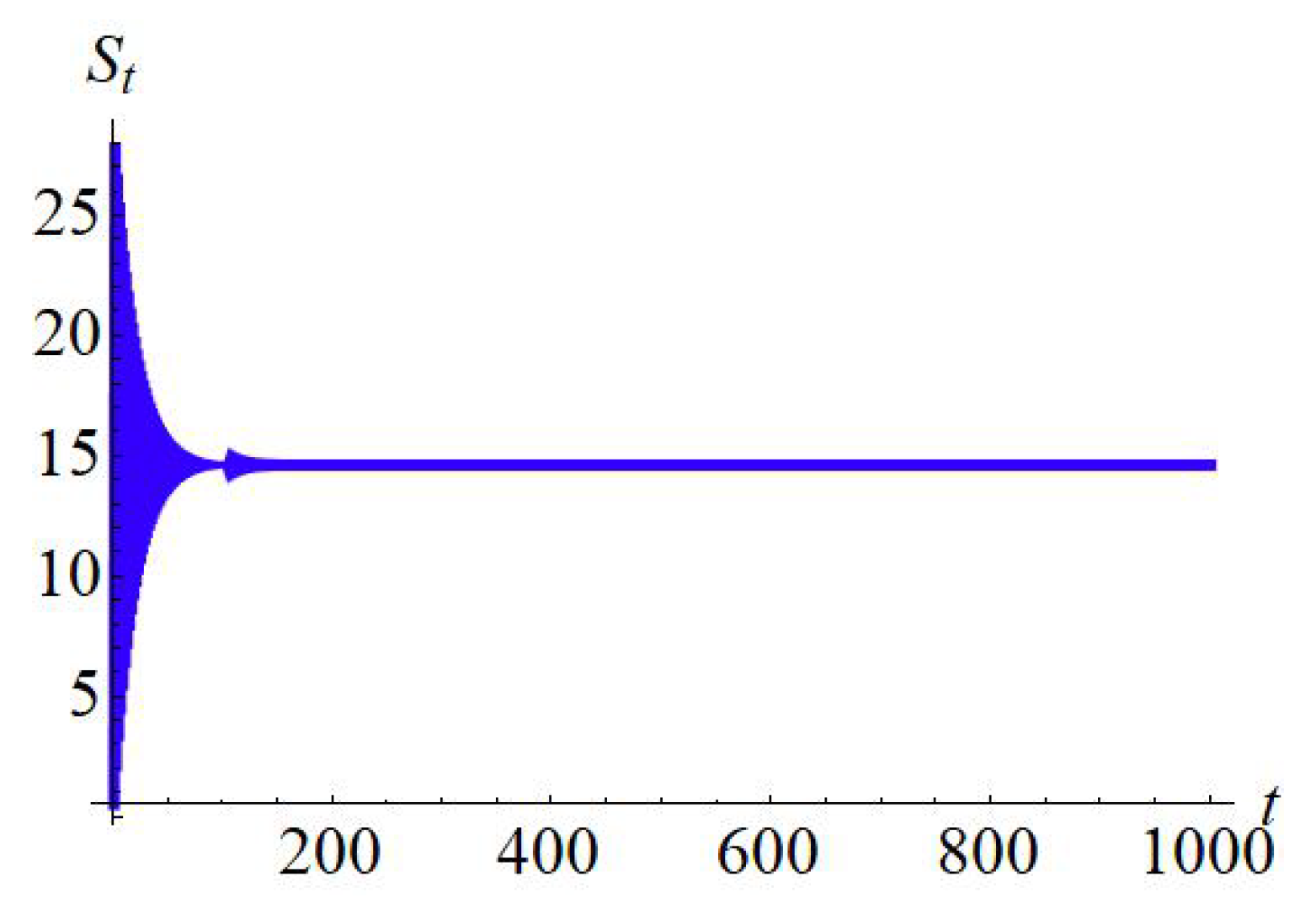
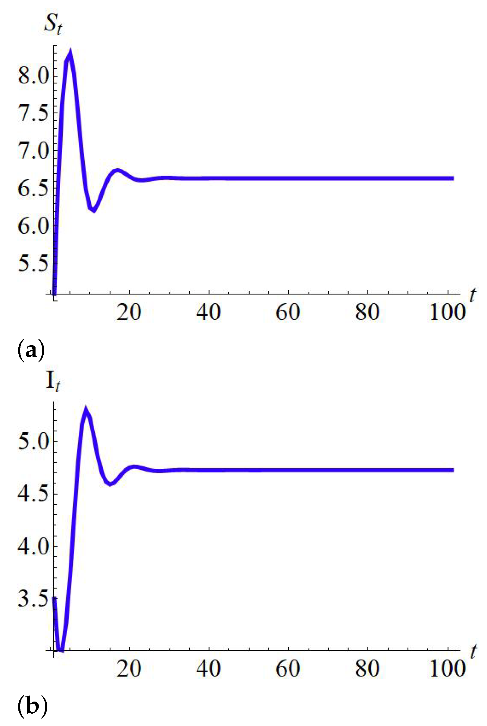
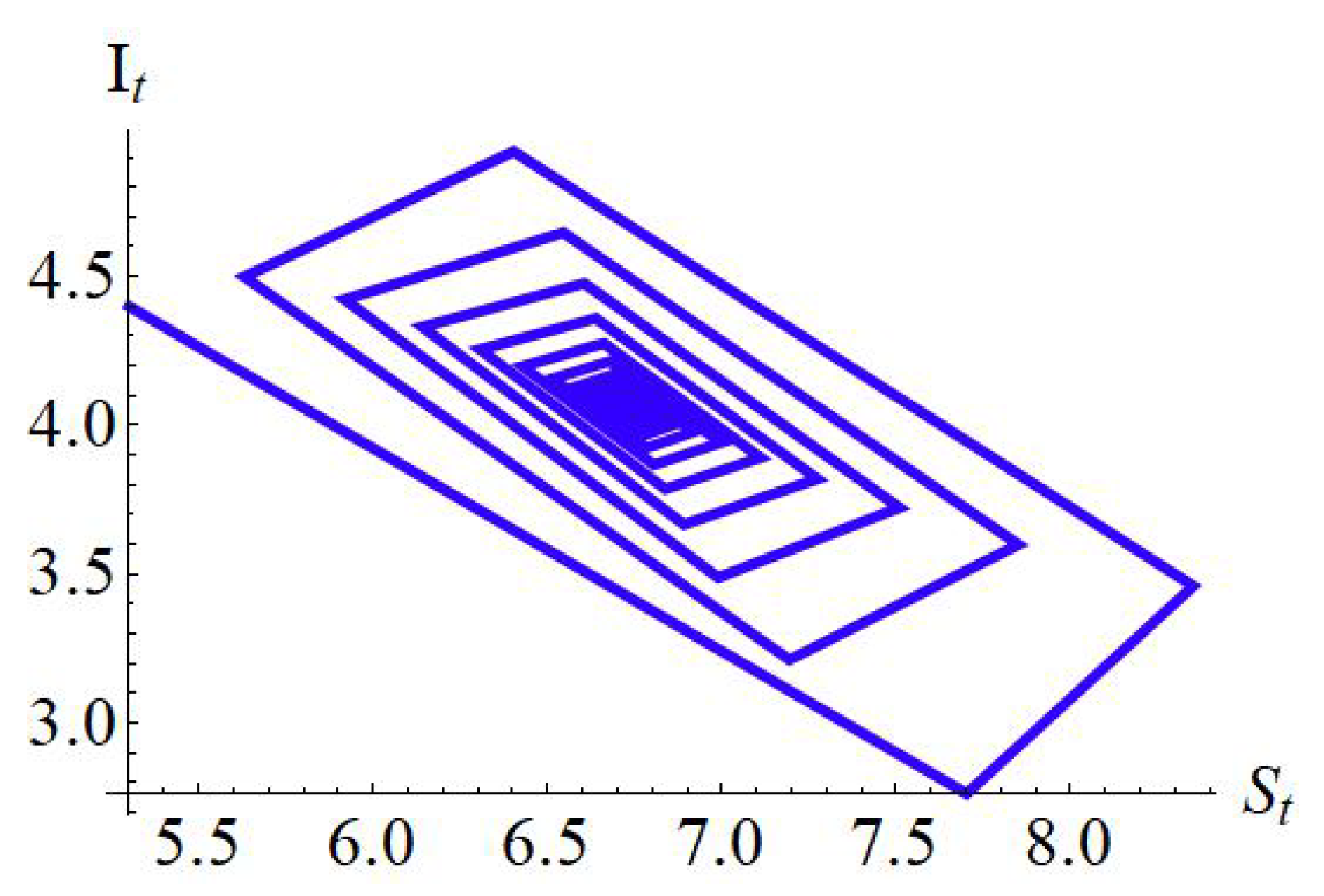
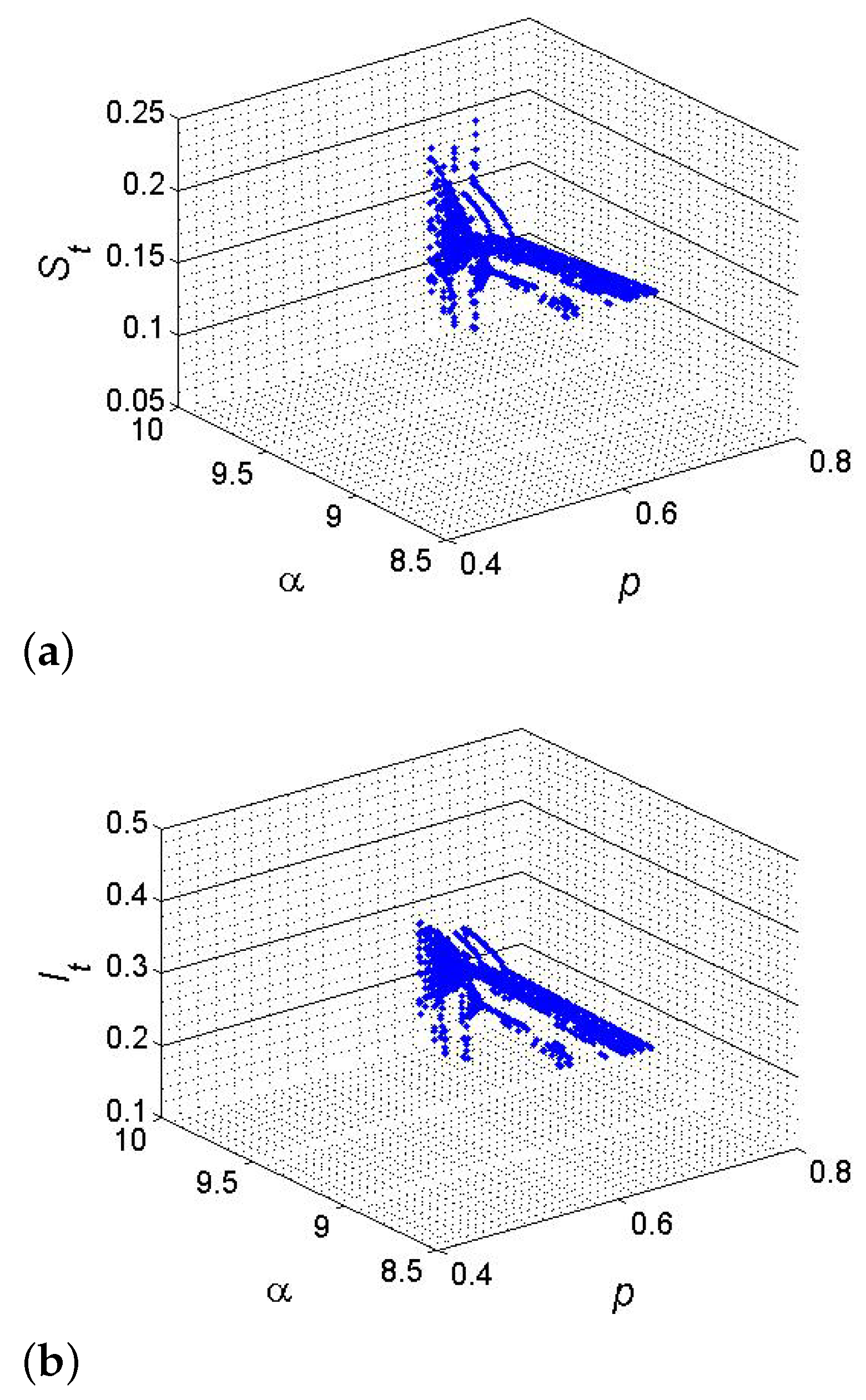
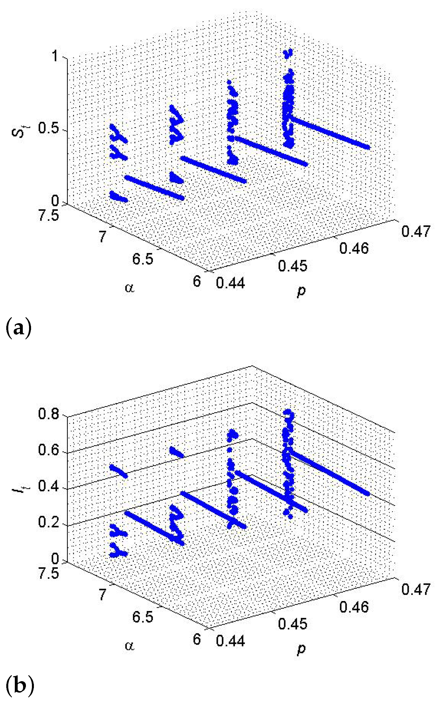
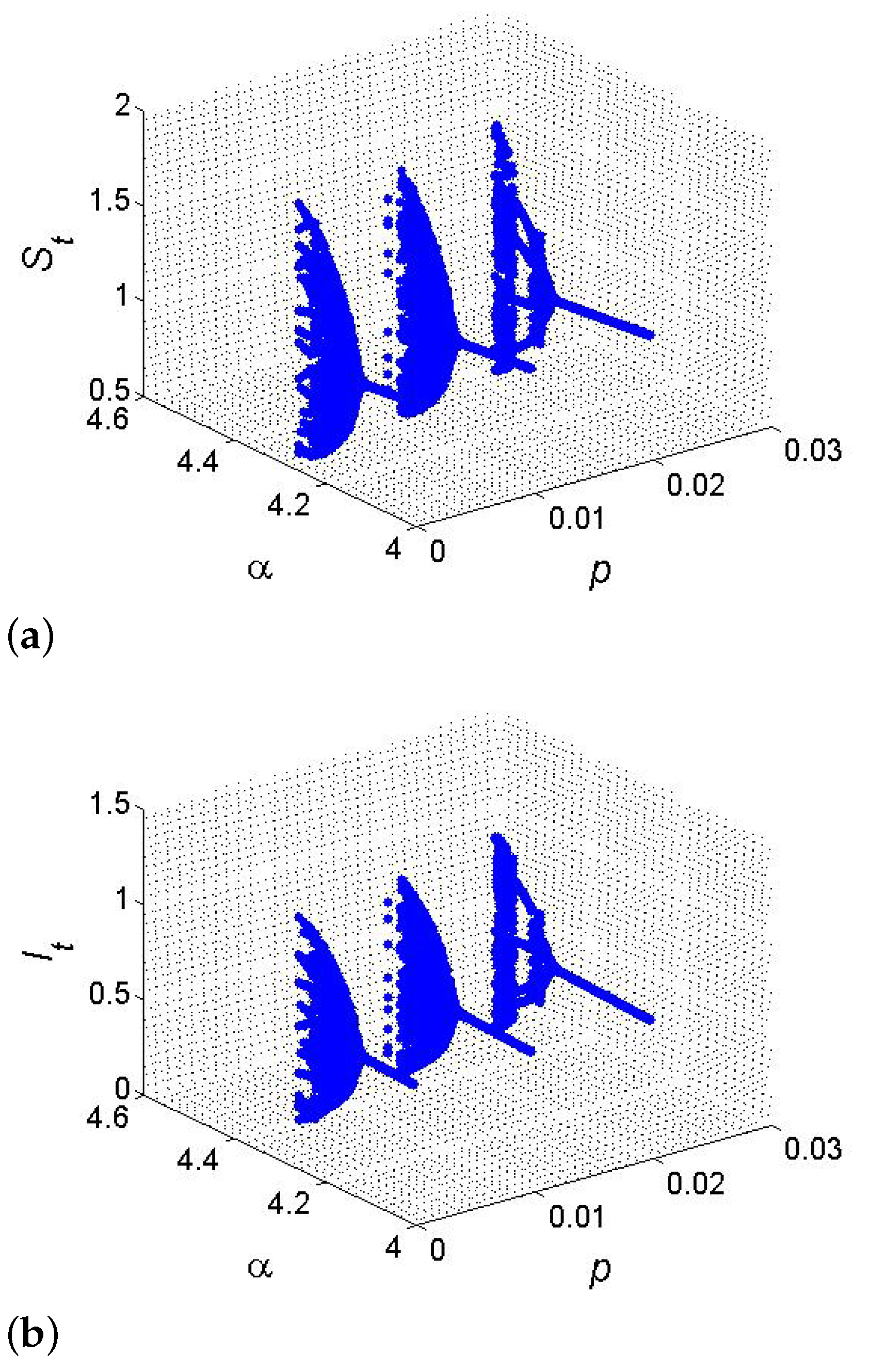
6. Numerical Simulations

The theory is numerically verified in this section.

Example 5.

If $p=0.05$, $N=15$, $\gamma =1.5$ and $\beta =1.9$, then from the parametric condition, which is depicted in (32), one has ${\displaystyle \frac{(p+\beta )\left((p+\beta )(\beta +\gamma -1)-\beta -\gamma \right)}{\beta (p+\beta -1)}}=1.38282548476425427<$$\alpha <\min \left\{{\displaystyle \frac{(p+\beta )\left(1+\beta +\gamma \right)+1}{\beta }},\right.\left.{\displaystyle \frac{(p+\beta )\left(3\beta +2\gamma +p-(p+\beta )\left(\beta +\gamma -1\right)-4\right)}{\beta (2-p-\beta )}}\right\}=\min \{5.042105263157895,$$1.4368421052631442\}=1.4368421052631442$ which implies that ${\Omega }_1$ of the SI model (12) is a sink if $\alpha \in \left(1.3828254847645427,1.43684210\right.\left.52631442\right)$. So, if $\alpha =1.39\in (1.3828254847645427,$$1.4368421052631442)$ then Figure 5 indicates that ${\Omega }_1=(14.615384615384617,0)$ is a sink.

Example 6.

If $p=0.1$, $N=45$, $\gamma =0.5$ and $\beta =0.09$, then from the parametric condition, which is depicted in (49), one has $\max \left\{{\displaystyle \frac{(p+\beta )(\beta +\gamma )}{\beta }},{\displaystyle \frac{(p+\beta ){(\beta +\gamma )}^2}{\beta (\beta +\gamma -1)}}\right\}$$=\max \{-1.792384823848238,$$1.245555555555555\}=1.245555555555555<\alpha <$${\displaystyle \frac{(\beta +\gamma )\left((p+\beta )(\beta +\gamma )-4\right)}{\beta (\beta +\gamma -2)}}$$=18.0761308116627$ which implies that ${\Omega }_2$ of SI model (12) is a sink if $\alpha \in (1.245555555555555,$$18.0761308116627)$. So, if $\alpha =4.0\in (1.245555555555555,$$18.0761308116627)$, then Figure 6 indicates that ${\Omega }_2=\left(6.63749999999999,4.72690677966101\right)$ is a sink.

Example 7.

If $p=0.05$, $N=15$, $\gamma =0.85$ and $\beta =0.9$, then from (55), one has the global condition $\max \left\{{\displaystyle \frac{{(\beta +\gamma )}^2}{\beta }},{\displaystyle \frac{(\beta +\gamma )(p+\beta )}{\beta }}\right\}=\max \left\{3.402777777777778,1.8472222222222223\right\}=$$3.402777777777778<\alpha <\min \left\{{\displaystyle \frac{(\beta +\gamma )(\beta +\gamma +2)}{\beta }},{\displaystyle \frac{(\beta +\gamma +2)(p+\beta )}{\beta }}\right\}=\min \{7.291666666666667,$$3.958333333333334\}=3.958333333333334$ which implies that ${\Omega }_2$ of te SI model (12) is globally stable if $\alpha \in \left(3.402777777777778,3.958333333333334\right)$. So, if $\alpha =3.9\in \left(3.402777777777778,3.958333333333334\right)$, then Figure 7 indicates that ${\Omega }_2=$$(6.730769230769232,4.060439560439559)$ is globally stable.

Example 8.

If $N=0.85$, $\beta =0.6$ and $\gamma =0.88$, then from (82), one gets $\alpha ={\displaystyle \frac{4(\beta +\gamma )}{\beta }}=9.866666666666667$ and $p={\displaystyle \frac{4(\beta +\gamma -1)}{\beta +\gamma }}-\beta =0.6972972972972973$. Furthermore, for said parametric values, the SI model (12) has a fixed point ${\Omega }_2=\left(0.1275,0.23283418553688823\right)$, where from (80), one gets ${\lambda }_{1,2}=-1$, and hence, for the existence of codimension-two bifurcation with 1:2 strong resonance, the eigenvalues criterion holds. Therefore, the set $\left(p,N,\alpha ,\beta ,\gamma \right)=\left(0.6972972972972973,0.85,9.866666666666667,0.6,0.88\right)\in {\mathcal{F}}_{12}{|}_{{\Omega }_2=\left(0.1275,0.23283418553688823\right)}$. But from (111), the simple manipulation yields that $C={\displaystyle \frac{16\left(3{\beta }^2+\beta (6\gamma -8)+3{\gamma }^2-8\gamma +4\right)}{{\beta }^2{N}^2}}=-78.04998077662438<0$, $D={\displaystyle \frac{16\left(7{\beta }^2+2\beta (7\gamma -6)+\gamma (7\gamma -12)+8\right)}{{\beta }^2{N}^2}}=342.80968858131496$, and $D+3C={\displaystyle \frac{64(\beta +\gamma -1)(4\beta +4\gamma -5)}{{\beta }^2{N}^2}}=108.65974625144176\ne 0$, which implies that at ${\Omega }_2=\left(0.1275,0.23283418553688823\right)$, the discrete-time SI model (12) undergoes a 1:2 strong resonance bifurcation if $\left(p,N,\alpha ,\beta ,\gamma \right)=\left(0.6972972972972973,0.85,9.866666666666667,0.6,0.88\right)\in {\mathcal{F}}_{12}{|}_{{\Omega }_2=\left(0.1275,0.23283418553688823\right)}$ which satisfies the conclusion of Theorem 11. Hence, 1:2 strong resonance bifurcation diagrams are drawn in Figure 8.

Example 9.

If $N=1.6$, $\beta =0.7$ and $\gamma =0.92$, then from (83), one gets $\alpha ={\displaystyle \frac{3(\beta +\gamma )}{\beta }}=6.942857142857143$ and $p={\displaystyle \frac{3(\beta +\gamma -1)}{\beta +\gamma }}-\beta =0.4481481481481482$. Furthermore, for said parametric values, the SI model (12) has a fixed point ${\Omega }_2=\left(0.3733333333,0.42676421277244325\right)$, where from (80), one gets ${\lambda }_{1,2}=0.4999999999999998\pm 0.8660254037844384\iota$, and hence, for the existence of codimension-two bifurcation with 1:3 strong resonance, the eigenvalues criterion holds. Therefore, the set $\left(p,N,\alpha ,\beta ,\gamma \right)=(0.4481481481481482,1.6,6.942857142857143,$$0.7,0.92)\in {\mathcal{F}}_{13}{|}_{{\Omega }_2=\left(0.3733333333,0.42676421277244325\right)}$. But from (130), one has $C={\displaystyle \frac{3(\beta +\gamma )}{8\beta N}}$$\left((6+2(\beta +\gamma ))+\iota \left(2(\beta +\gamma )+3+\sqrt{3}\right)\right)=0.5011875+0.432412577285544\iota$ and $D=$${\displaystyle \frac{9{(\beta +\gamma )}^2}{8{\beta }^2{N}^2}}\left(7{(\beta +\gamma )}^2-24(\beta +\gamma )+24+\iota \left(\sqrt{3}{(\beta +\gamma )}^2-8\sqrt{3}(\beta +\gamma )\right)\right)=0.08216208912627555-$$0.42134983366861994\iota$. Finally, from (131), one gets $C_1=-{\displaystyle \frac{9(\beta +\gamma )}{16\beta N}}\times \left(2(1-\sqrt{3})(\beta +\gamma )+3(1-\sqrt{3})+\iota \left(2(1+\sqrt{3})(\beta +\gamma )+(3+7\sqrt{3})\right)\right)$$=0.37165958053554915-1.9507421871059567\iota \ne 0$ and $D_1=-{\displaystyle \frac{27{(\beta +\gamma )}^2}{32{\beta }^2{N}^2}}\left(12{(\beta +\gamma )}^2+2(9+\sqrt{3})(\beta +\gamma )+72+3\sqrt{3}+\iota \left(16\sqrt{3}{(\beta +\gamma )}^2+64\sqrt{3}(\beta +\gamma )+12\sqrt{3}\right)\right)$$=-2.532450754654462-4.8207939172228595\iota$ where $\Re \left(D_1\right)=-2.532450754654462<0$ imply that at ${\Omega }_2=(0.3733333333,$$0.42676421277244325)$, model (12) undergoes a 1:3 strong resonance bifurcation if $\left(p,N,\alpha ,\beta ,\gamma \right)=(0.4481481481481482,1.6,$$6.942857142857143,0.7,0.92)\in$${\mathcal{F}}_{13}{|}_{{\Omega }_2=\left(0.3733333333,0.42676421277244325\right)}$, which satisfies the conclusion of Theorem 12. Hence, 1:3 strong resonance bifurcation diagrams are drawn in Figure 9.

Example 10.

If $N=2.7$, $\beta =0.8$ and $\gamma =0.9$, then from (84), one gets $\alpha ={\displaystyle \frac{2(\beta +\gamma )}{\beta }}=4.25$ and $p={\displaystyle \frac{2(\beta +\gamma -1)}{\beta +\gamma }}-\beta =0.02352941176470602$. Furthermore, for said parametric values, the SI model (12) has a fixed point ${\Omega }_2=\left(1.08,0.7474048442906572\right)$, where from (80), one gets ${\lambda }_{1,2}=\pm \iota$, and hence, for the existence of codimension-two bifurcation with 1:4 strong resonance, the eigenvalues criterion holds. Therefore, the set $\left(p,N,\alpha ,\beta ,\gamma \right)=\left(0.06666666666666665,0.7,5.0,0.6,0.9\right)\in {\mathcal{F}}_{14}{|}_{{\Omega }_2=\left(1.08,0.7474048442906572\right)}$. But from (143), the simple manipulation yields that $C={\displaystyle \frac{{(\beta +\gamma )}^2}{2{\beta }^2{N}^2}}{\times (5(\beta +\gamma )}^2-13(\beta +\gamma )+2+\iota (-9{(\beta +\gamma )}^2+$$12(\beta +\gamma )-2\left)\right)=-1.7498821159122078-2.3569208676268865\iota$, $D=-{\displaystyle \frac{{(\beta +\gamma )}^2}{2{\beta }^2{N}^2}}(2(\beta +\gamma )+$$\iota (2-{(\beta +\gamma )}^2))=-1.053026406035665+0.2756451474622772\iota$, moreover, from (144), one gets $C_1=-{\displaystyle \frac{2{(\beta +\gamma )}^2}{{\beta }^2{N}^2}}\left(9{(\beta +\gamma )}^2-12(\beta +\gamma )+2+\iota \left(5{(\beta +\gamma )}^2-13(\beta +\gamma )+2\right)\right)=-9.427683470507546+6.999528463648831\iota \ne 0$, $D_1={\displaystyle \frac{2{(\beta +\gamma )}^2}{{\beta }^2{N}^2}}\left({(\beta +\gamma )}^2-2+2(\beta +\gamma )\iota \right)=1.1025805898491088+4.21210562414266\iota \ne 0$. Finally, from (145), one gets $B=-{\displaystyle \frac{\sqrt{2}(\beta +\gamma )}{\beta N\sqrt{{(\beta +\gamma )}^4+4}}}\left(9{(\beta +\gamma )}^2-12(\beta +\gamma )+2)+\left(5{(\beta +\gamma )}^2-13(\beta +\gamma )+2\right)\iota \right)=-4.097069647399329+3.041845401814218\iota$ where $\Re \left(B\right)=-4.097069647399329\ne 0$ and $\Im \left(B\right)=3.041845401814218\ne 0$, which implies that at ${\Omega }_2=\left(1.08,0.7474048442906572\right)$, the discrete-time SI model (12) undergoes a 1:4 strong resonance bifurcation if $\left(p,N,\alpha ,\beta ,\gamma \right)=\left(0.06666666666666665,0.7,5.0,0.6,0.9\right)\in {\mathcal{F}}_{14}{|}_{{\Omega }_2=\left(1.08,0.7474048442906572\right)}$, which satisfies the conclusion of Theorem 13. Hence, 1:4 strong resonance bifurcation diagrams are drawn in Figure 10.

7. Conclusions

This work is about the global dynamics and codimension-two bifurcation analysis of a discrete epidemic model (12) that describes the spread of an infectious disease within a closed population. More precisely, it is proved that if $p<\gamma$ and $p+\beta <1$, then the solution ${\left\{\left(S_t,I_t\right)\right\}}_{t=0}^{\infty }$ of the SI model (12) is bounded, which implies biologically that when vaccination efforts are insufficient to outpace the recovery of individual I, the disease burden remains constrained, but it does not necessarily disappear. Furthermore, the set $\left[0,{\displaystyle \frac{\beta N}{p+\beta }}\right]\times \left[0,{\displaystyle \frac{\beta N}{p+\beta }}\right]$ is an invariant set, suggesting that the maximum number of individuals S and I in the population depends on the birth and vaccination rates $\beta$ and p, respectively. This emphasizes the role of vaccination in controlling outbreaks, as increasing p reduces the population S, thereby depressing the risk of the spread of disease. We then constructed the linearized system at a fixed point of the SI model (12). By the theory of linear stability, it is proved that ${\Omega }_1$ is a sink if the contact rate $\alpha$ lies within a specific range, that is, ${\displaystyle \frac{(p+\beta )\left((p+\beta )(\beta +\gamma -1)-\beta -\gamma \right)}{\beta (p+\beta -1)}}<\alpha <\min \left\{{\displaystyle \frac{(p+\beta )\left(1+\beta +\gamma \right)+1}{\beta }},{\displaystyle \frac{(p+\beta )\left(3\beta +2\gamma +p-(p+\beta )\left(\beta +\gamma -1\right)-4\right)}{\beta (2-p-\beta )}}\right\}$, which means that if the rate of transmission is sufficiently low, any introduced infection will eventually disappear, emphasizing the importance of reducing contact rate $\alpha$ through public health interventions, such as quarantine and social distancing (source: if ${\displaystyle \frac{(p+\beta )\left((p+\beta )(\beta +\gamma -1)+\beta +\gamma +2\right)}{\beta (p+\beta -1)}}<\alpha <\min \left\{{\displaystyle \frac{(p+\beta )\left(1+\beta +\gamma \right)+1}{\beta }},{\displaystyle \frac{(p+\beta )\left(3\beta +2\gamma +p-(p+\beta )\left(\beta +\gamma -1\right)-4\right)}{\beta (2-p-\beta )}}\right\}$ means leading to disease outbreaks, saddle if ${\displaystyle \frac{(p+\beta )(\gamma -p)}{\beta }}<\alpha <{\displaystyle \frac{(p+\beta )\left(3\beta +2\gamma +p-(p+\beta )\left(\beta +\gamma -1\right)-4\right)}{\beta (2-p-\beta )}}$, and nonhyperbolic if one has the condition $\alpha ={\displaystyle \frac{(p+\beta )\left(3\beta +2\gamma +p-(p+\beta )\left(\beta +\gamma -1\right)-4\right)}{\beta (2-p-\beta )}}$). We have also derived the sufficient condition, that is, $\alpha >{\displaystyle \frac{(p+\beta )\left(3\beta +2\gamma +p-(p+\beta )\left(\beta +\gamma -1\right)-4\right)}{\beta (2-p-\beta )}}$ under which ${\Omega }_1$ is a sink. Furthermore, it was also proved that ${\Omega }_2$ is a sink if $\max \left\{{\displaystyle \frac{(p+\beta )(\beta +\gamma )}{\beta }},{\displaystyle \frac{(p+\beta ){(\beta +\gamma )}^2}{\beta (\gamma +\beta -1)}}\right\}<\alpha <{\displaystyle \frac{(\beta +\gamma )\left((p+\beta )(\beta +\gamma )-4\right)}{\beta (\gamma +\beta -2)}}$, which suggests that the disease becomes endemic despite control measures. This theoretical finding highlights the need for enhanced treatment protocols and vaccination campaigns to diminish transmission and push the system to extinction (source: if one holds the parametric condition ${\displaystyle \frac{(p+\beta )(\beta +\gamma )}{\beta }}<\alpha <\min \left\{{\displaystyle \frac{(\beta +\gamma )\left((p+\beta )(\beta +\gamma )-4\right)}{\beta (\gamma +\beta -2)}},{\displaystyle \frac{(\beta +\gamma )\left((p+\beta )(\beta +\gamma )-2\right)}{\beta (\gamma +\beta -1)}}\right\}$, which can be interpreted as unpredictable or periodic outbreaks epidemic patterns, nonhyperbolic if $\alpha ={\displaystyle \frac{(p+\beta )(\beta +\gamma )}{\beta }},$ or $\alpha ={\displaystyle \frac{(\gamma +\beta )\left((p+\beta )(\beta +\gamma )-4\right)}{\beta (\gamma +\beta -2)}}$, saddle if $\max \left\{{\displaystyle \frac{2(\gamma +\beta )\left(\gamma +\beta +\sqrt{(\beta +\gamma )(\gamma -p)}\right)}{\beta }},{\displaystyle \frac{2(\gamma +\beta )\left(\gamma +\beta -\sqrt{(\beta +\gamma )(\gamma -p)}\right)}{\beta }}\right\}<\alpha <{\displaystyle \frac{(\gamma +\beta )\left(\right(p+\beta \left)\right(\beta +\gamma )-4)}{\beta (\gamma +\beta -2)}},$, and finally, one has the condition $\alpha <{\displaystyle \frac{(\gamma +\beta )(4-(p+\beta \left)\right(\beta +\gamma \left)\right)}{\beta (2-\beta -\gamma )}}$, where ${\Omega }_2$ is a sink). We then studied the global dynamics and proved that ${\Omega }_1$ is a global attractor if $\alpha <{\displaystyle \frac{(\beta +\gamma )(p+\beta )}{\beta }}$, which implies that if the rate of transmission is kept below a threshold, then the disease will be eliminated regardless of the initial conditions. Also, ${\Omega }_2$ is a global attractor if $\max \left\{{\displaystyle \frac{{(\beta +\gamma )}^2}{\beta }},{\displaystyle \frac{(\beta +\gamma )(\beta +p)}{\beta }}\right\}<\alpha <\min \left\{{\displaystyle \frac{(\beta +\gamma )(2+\beta +\gamma )}{\beta }},{\displaystyle \frac{(\beta +p)(\beta +\gamma +2)}{\beta }}\right\}$, meaning that disease persistence is inevitable. This highlights the importance of early intervention strategies such as improved healthcare infrastructure, mass vaccination, and public awareness campaigns to keep the rate of transmission low and then drive the system toward a disease-free state. Additionally, for the study of complex dynamics, we have also first identified two-parameter bifurcation sets, that is, (i) 1:2 strong resonance set ${\mathcal{F}}_{12}{|}_{{\Omega }_2}=\left\{\left(p,N,\alpha ,\beta ,\gamma \right):\alpha ={\displaystyle \frac{4(\beta +\gamma )}{\beta }},p={\displaystyle \frac{4(\beta +\gamma -1)}{\beta +\gamma }}-\beta \right\}$, (ii) 1:3 strong resonance set ${\mathcal{F}}_{13}{|}_{{\Omega }_2}=\left\{\left(p,N,\alpha ,\beta ,\gamma \right):\alpha ={\displaystyle \frac{3(\beta +\gamma )}{\beta }},p={\displaystyle \frac{3(\beta +\gamma -1)}{\beta +\gamma }}-\beta \right\}$, and (iii) 1:4 strong resonance set ${\mathcal{F}}_{14}{|}_{{\Omega }_2}=\left\{\left(p,N,\alpha ,\beta ,\gamma \right):\alpha ={\displaystyle \frac{2(\beta +\gamma )}{\beta }},p={\displaystyle \frac{2(\beta +\gamma -1)}{\beta +\gamma }}-\beta \right\}$, and then detail two-parameter bifurcation analysis is given by series of affine transformations and bifurcation theory. The occurrence of two-parameter bifurcations indicates that under derivable parameter conditions, the SI model (12) may exhibit complex behaviors such as chaotic fluctuations or periodic oscillations in infection levels. Biologically, this implies that certain epidemiological scenarios could lead to cyclic epidemics, where the level of infection falls and rises in an irregular or regular manner. Such findings are particularly relevant for diseases with seasonal transmission patterns or those affected by varying environmental conditions. Finally, theoretical results are validated numerically, where the numerical simulation section includes two-parameter bifurcation diagrams, time series graphs, global attractor, and region of stability in two and three-dimensional parametric space accordingly.

Future Work

Dynamical analysis of a discrete SI model (12) with complex network and stochastic modeling is our next aim.

References

1. Nii-Trebi, N.I. Emerging and neglected infectious diseases: Insights, advances, and challenges. BioMed Res. Int. 2017, 2017, 5245021. [Google Scholar] [CrossRef] [PubMed]
2. Church, D.L. Major factors affecting the emergence and re-emergence of infectious diseases. Clin. Lab. Med. 2004, 24, 559–586. [Google Scholar] [CrossRef] [PubMed]
3. Frank, S.A. Immunology and Evolution of Infectious Disease; Princeton University Press: Princeton, NJ, USA, 2002. [Google Scholar]
4. Li, M.Y. An Introduction to Mathematical Modeling of Infectious Diseases; Springer: Cham, Switzerland, 2018. [Google Scholar]
5. Cohen, J.; Powderly, W.G.; Opal, S.M. Infectious Diseases E-Book; Elsevier Health Sciences: New York, NY, USA, 2016. [Google Scholar]
6. Elaydi, S.N.; Cushing, J.M. Discrete Mathematical Models in Population Biology: Ecological, Epidemic, and Evolutionary Dynamics; Springer Nature: New York, NY, USA, 2024. [Google Scholar]
7. Giles, P. The mathematical theory of infectious diseases and its applications. J. Oper. Res. Soc. 1977, 28, 479–480. [Google Scholar] [CrossRef]
8. Vynnycky, E.; White, R. An Introduction to Infectious Disease Modelling; OUP Oxford: Oxford, UK, 2010. [Google Scholar]
9. Frauenthal, J.C. Mathematical Modeling in Epidemiology; Springer Science & Business Media: New York, NY, USA, 2012. [Google Scholar]
10. Huppert, A.; Katriel, G. Mathematical modelling and prediction in infectious disease epidemiology. Clin. Microbiol. Infect. 2013, 19, 999–1005. [Google Scholar] [CrossRef] [PubMed]
11. Strogatz, S.H. Nonlinear Dynamics and Chaos: With Applications to Physics, Biology, Chemistry, and Engineering; Westview Press: Boulder, CO, USA, 2001. [Google Scholar]
12. Hilborn, R.C. Chaos and Nonlinear Dynamics: An Introduction for Scientists and Engineers; Oxford University Press: Oxford, UK, 2000. [Google Scholar]
13. Allen, L.J. An Introduction to Stochastic Processes with Applications to Biology; CRC Press: Boca Raton, FL, USA, 2010. [Google Scholar]
14. Brauer, F.; Castillo-Chavez, C.; Castillo-Chavez, C. Mathematical Models in Population Biology and Epidemiology; Springer: New York, NY, USA, 2012. [Google Scholar]
15. Roberts, M.G.; Heesterbeek, J.A.P. Mathematical Models in Epidemiology; EOLSS: Abu Dhabi, United Arab Emirates, 2003. [Google Scholar]
16. Parsamanesh, M.; Erfanian, M.; Mehrshad, S. Stability and bifurcations in a discrete-time epidemic model with vaccination and vital dynamics. BMC Bioinform. 2020, 21, 525. [Google Scholar] [CrossRef] [PubMed]
17. Parsamanesh, M.; Erfanian, M. Global dynamics of an epidemic model with standard incidence rate and vaccination strategy. Chaos Solitons Fractals 2018, 117, 192–199. [Google Scholar] [CrossRef]
18. Chen, Y.; Wen, B.; Teng, Z. The global dynamics for a stochastic SIS epidemic model with isolation. Phys. A Stat. Mech. Its Appl. 2018, 492, 1604–1624. [Google Scholar] [CrossRef] [PubMed]
19. Cui, J.A.; Zhao, S.; Guo, S.; Bai, Y.; Wang, X.; Chen, T. Global dynamics of an epidemiological model with acute and chronic HCV infections. Appl. Math. Lett. 2020, 103, 106203. [Google Scholar] [CrossRef]
20. Darti, I.; Suryanto, A.; Hartono, M. Global stability of a discrete SIR epidemic model with saturated incidence rate and death induced by the disease. Commun. Math. Biol. Neurosci. 2020, 2020, 33. [Google Scholar]
21. Li, T.; Zhang, F.; Liu, H.; Chen, Y. Threshold dynamics of an SIRS model with nonlinear incidence rate and transfer from infectious to susceptible. Appl. Math. Lett. 2017, 70, 52–57. [Google Scholar] [CrossRef]
22. Hu, D.; Liu, X.; Li, K.; Liu, M.; Yu, X. Codimension-two bifurcations of a simplified discrete-time SIR model with nonlinear incidence and recovery rates. Mathematics 2023, 11, 4142. [Google Scholar] [CrossRef]
23. Eskandari, Z.; Alidousti, J. Stability and codimension-2 bifurcations of a discrete time SIR model. J. Frankl. Inst. 2020, 357, 10937–10959. [Google Scholar] [CrossRef]
24. Ruan, M.; Li, C.; Li, X. Codimension two 1:1 strong resonance bifurcation in a discrete predator-prey model with Holling IV functional response. AIMS Math. 2021, 7, 3150–3168. [Google Scholar] [CrossRef]
25. Abdelaziz, M.A.; Ismail, A.I.; Abdullah, F.A.; Mohd, M.H. Codimension-one and two bifurcations of a discrete-time fractional-order SEIR measles epidemic model with constant vaccination. Chaos Solitons Fractals 2020, 140, 110104. [Google Scholar] [CrossRef]
26. Yi, N.; Zhang, Q.; Liu, P.; Lin, Y. Codimension-two bifurcations analysis and tracking control on a discrete epidemic model. J. Syst. Sci. Complex. 2011, 24, 1033–1056. [Google Scholar] [CrossRef]
27. Khan, A.Q.; Akhtar, T.; Jhangeer, A.; Riaz, M.B. Codimension-two bifurcation analysis at an endemic equilibrium state of a discrete epidemic model. AIMS Math. 2024, 9, 13006–13027. [Google Scholar] [CrossRef]
28. Allen, L.J. An Introduction to Mathematical Biology; Pearson Prentice Hall: Upper Saddle River, NJ, USA, 2007. [Google Scholar]
29. Grove, E.A.; Ladas, G. Periodicities in Nonlinear Difference Equations; Chapman and Hall/CRC: Boca Raton, FL, USA, 2004. [Google Scholar]
30. Kulenović, M.R.S.; Ladas, G. Dynamics of Second-Order Rational Difference Equations: With Open Problems and Conjectures; Chapman and Hall/CRC: Boca Raton, FL, USA, 2001. [Google Scholar]
31. Camouzis, E.; Ladas, G. Dynamics of Third-Order Rational Difference Equations with Open Problems and Conjectures; CRC Press: Boca Raton, FL, USA, 2007. [Google Scholar]
32. Guckenheimer, J.; Holmes, P. Nonlinear Oscillations, Dynamical Systems, and Bifurcations of Vector Fields; Springer Science & Business Media: New York, NY, USA, 2013. [Google Scholar]
33. Kuznetsov, Y.A.; Kuznetsov, I.A.; Kuznetsov, Y. Elements of Applied Bifurcation Theory; Springer: New York, NY, USA, 1998. [Google Scholar]
34. Liu, X.; Liu, Y. Codimension-two bifurcation analysis on a discrete Gierer-Meinhardt system. Int. J. Bifurc. Chaos 2020, 30, 2050251. [Google Scholar] [CrossRef]
35. Wiggins, S. Introduction to Applied Nonlinear Dynamical System and Chaos; Springer: New York, NY, USA, 2003. [Google Scholar]
36. Wu, X.P.; Wang, L. Analysis of oscillatory patterns of a discrete-time Rosenzweig-MacArthur model. Int. J. Bifurc. Chaos 2018, 28, 1850075. [Google Scholar] [CrossRef]
37. Wikan, A. Discrete Dynamical Systems with an Introduction to Discrete Optimization Problems; Bookboon.com: London, UK, 2013. [Google Scholar]
Figure 1. Dynamics of Ω 1 with α ( 0.0 , 2.5 ) and p ( 0.0 , 1.1 ) .
Axioms 14 00463 g001
Figure 2. Dynamics of Ω 1 with p ( 0.0 , 1.0 ) , γ ( 1.0 , 3.3 ) and α ( 1.5 , 3.0 ) .
Axioms 14 00463 g002
Figure 3. Dynamics of Ω 2 with p ( 0.1 , 1.0 ) and α ( 0.0 , 5.5 ) .
Axioms 14 00463 g003
Figure 4. Dynamics of Ω 2 with p ( 0.1 , 1.5 ) , γ ( 0.3 , 1.5 ) and α ( 1.9 , 5.9 ) .
Axioms 14 00463 g004
Figure 5. Local dynamics at Ω 1 = ( 14.615384615384617 , 0 ) of the SI model (12).
Axioms 14 00463 g005
Figure 6. (a) Plot of t vs. S t ; (b) Plot of t vs. I t . Local dynamics at Ω 2 = ( 6.63749999999999 , 4.72690677966101 ) of the SI model (12).
Axioms 14 00463 g006
Figure 7. Global dynamics at Ω 2 = ( 6.730769230769232 , 4.060439560439559 ) of the SI model (12).
Axioms 14 00463 g007
Figure 8. (a) Plot for p, α and S t ; (b) Plot for p, α and I t . A 1:2 strong resonance bifurcation diagram if p , N , α , β , γ = ( 0.6972972972972973 , 0.85 , 9.866666666666667 , 0.6 , 0.88 ) F 12 | Ω 2 = 0.1275 , 0.23283418553688823 .
Axioms 14 00463 g008
Figure 9. (a) Plot for p, α and S t ; (b) Plot for p, α and I t . A 1:3 strong resonance bifurcation diagram if p , N , α , β , γ = ( 0.4481481481481482 , 1.6 , 6.942857142857143 , 0.7 , 0.92 ) F 13 | Ω 2 = 0.3733333333 , 0.42676421277244325 .
Axioms 14 00463 g009
Figure 10. (a) Plot for p, α and S t ; (b) Plot for p, α and I t . A 1:4 strong resonance bifurcation diagram if p , N , α , β , γ = ( 0.06666666666666665 , 0.7 , 5.0 , 0.6 , 0.9 ) F 14 | Ω 2 = 1.08 , 0.7474048442906572 .
Axioms 14 00463 g010
Disclaimer/Publisher’s Note: The statements, opinions and data contained in all publications are solely those of the individual author(s) and contributor(s) and not of MDPI and/or the editor(s). MDPI and/or the editor(s) disclaim responsibility for any injury to people or property resulting from any ideas, methods, instructions or products referred to in the content.