Mode Locking, Farey Sequence, and Bifurcation in a Discrete Predator-Prey Model with Holling Type IV Response

Abstract

This paper presents and examines a discrete-time predator–prey model of the Leslie type, integrating a Holling type IV functional response for analysis. The mathematical analysis succinctly identifies fixed points and evaluates their local stability within the model. The study employs the normal form approach and bifurcation theory to explore codimension-one and two bifurcation behaviors for this model. The primary conclusions are substantiated by a combination of rigorous theoretical analysis and meticulous computational simulations. Additionally, utilizing fractal basin boundaries, periodicity variations, and Lyapunov exponent distributions within two-parameter spaces, we observe a mode-locking structure akin to Arnold tongues. These periods are arranged in a Farey tree sequence and embedded within quasi-periodic/chaotic regions. These findings enhance comprehension of bifurcation cascade emergence and structural patterns in diverse biological systems with discrete dynamics.

1. Introduction

Predator–prey dynamics remain a cornerstone of ecological modeling, with enduring relevance to the field. Recent advancements have refined traditional frameworks, yielding a wealth of novel insights through published studies [1,2,3,4,5,6]. Among these diverse models, ecological researchers and mathematical scientists have rigorously explored those models incorporating Holling-type functional responses, driving deep theoretical and empirical insights. The functional response is the specific growth rate representing the prey consumption per unit time, which describes how the rate at which predators consume prey changes with prey abundance. Proposed by ecologist C.S. Holling [7], these models categorize predation rates into three main types—Holling type II [8,9], Holling type III [10,11], and Holling type IV [12,13]—and they bridge empirical observations with theoretical models, enabling ecologists to predict and manage ecosystems more effectively. Qualitative analyses of these studies have revealed rich dynamics, including limit cycles, stable states, Hopf bifurcations, fold bifurcations, Bogdanov–Takens bifurcations of codimension-two and codimension-three, etc. While prior works have predominantly centered on predator–prey dynamics modeled by ordinary differential equations (ODEs), there is a growing enthusiasm among modern researchers for discrete-time difference equation frameworks.

It is widely recognized that discrete-time models are particularly suited for studying the evolutionary behavior of species or taxonomic groups with clearly defined developmental stages and nonoverlapping generations. Furthermore, mathematical models are often inferred from biological and chemical measurements acquired at discrete temporal and spatial scales. Consequently, discrete-time models present a superior alternative to continuous models by enabling more direct formulation, efficient simulation, and enhanced fidelity to empirical observations. As a result, there has been growing interest in discrete models in recent years, especially concerning codimension-two bifurcations [14,15,16]. Yuan and Yang [14] demonstrated that a traditional discrete predator–prey system exhibited a 1:2 strong resonance in addition to codimension-one bifurcations. Li and He [15] explored the bifurcation dynamics of a discrete Hindmarsh–Rose system with two controlling parameters, uncovering coexisting 1:2 and 1:4 resonances within the system. Zhang et al. [16] deciphered the codimension-two bifurcation in a discrete predator–prey model, revealing its intricate linkage with 1:2 resonance and lower-order codimension-one bifurcations. Our primary objective is to report on the codimension-two bifurcations in a discrete-time difference model, focusing on their coupling with 1:2, 1:3, and 1:4 resonance phenomena.

In [17], Sohel Rana and Kulsum developed a Leslie-type predator–prey model incorporating a simplified Holling type IV functional response, which is expressed as

$$\left\{\begin{array}{c}{\displaystyle \frac{dx}{d\tau }}=rx\left(1-{\displaystyle \frac{x}{k}}\right)-{\displaystyle \frac{mxy}{x^2+b}},\hfill \\ {\displaystyle \frac{dy}{d\tau }}=sy\left(1-{\displaystyle \frac{y}{hx}}\right),\hfill \end{array}\right.$$

(1)

where x and y denote prey and predator densities, k represents the carrying capacity, r denotes the intrinsic growth rate of the prey in the absence of predation, and h quantifies the preys food quality for converting into predator births. The parameter s corresponds to the predators’ intrinsic growth rate, while the term $mx/(x^2+b)$ embodies a simplified Holling type IV functional response. All parameters are positive constants.

To simplify the model, we nondimensionalize the variables and parameters as follows:

$${\displaystyle \frac{x}{k}}\to x,{\displaystyle \frac{my}{r{k}^2}}\to y,t=r\tau ,a={\displaystyle \frac{b}{k^2}},\alpha ={\displaystyle \frac{s}{r}},\beta ={\displaystyle \frac{sk}{hm}}.$$

We then reformulate system (1) as follows:

$$\left\{\begin{array}{c}{\displaystyle \frac{dx}{dt}}=x\left(1-x\right)-{\displaystyle \frac{xy}{x^2+a}},\hfill \\ {\displaystyle \frac{dy}{dt}}=y\left(\alpha -{\displaystyle \frac{\beta y}{x}}\right).\hfill \end{array}\right.$$

(2)

Solving a complex differential equation without a computer is challenging, so one effective strategy involves employing discretization techniques to derive and analyze a corresponding discrete-time system. This analysis aids in elucidating the characteristics of the underlying continuous system. Discretizing a complex differential equation can be accomplished using tailored numerical approaches, including the forward Euler method for explicit time integration, the backward Euler method for implicit stability, or semidiscretization to handle spatial derivatives while retaining temporal continuousness. The choice depends on the equation’s stiffness, accuracy requirements, and computational constraints. Here, the forward Euler method is applied to derive the discrete model of system (2). As the most straightforward discretization approach, it transforms continuous differential equations into a difference scheme. However, its explicit nature limits stability for large time steps, especially compared to higher-order or implicit methods like backward Euler or Runge–Kutta. The forward Euler method is applied to system (2), yielding the following discrete form:

$$\left(\begin{array}{c}x\\ y\end{array}\right)\to \left(\begin{array}{c}x+\delta x\left[(1-x)-{\displaystyle \frac{y}{x^2+a}}\right]\\ y+\delta y(\alpha -{\displaystyle \frac{\beta y}{x}})\end{array}\right),$$

(3)

where $\delta >0$ represents the integral step size. In Ref. [17], the authors employed center manifold theory to analyze codimension-one bifurcations in model (3), focusing on flip and Neimark–Sacker bifurcations. All numerical simulations and analytical results were considered under the variation of at most one parameter. Building on prior work, we investigate the high-order bifurcations of model (3), specifically codimension-two cases like 1:2, 1:3, and 1:4 resonances. The emergence conditions for these bifurcations are systematically characterized. Numerical simulations, comprising bifurcation diagrams, phase portraits, and Lyapunov exponents, are employed to validate theoretical predictions and reveal emergent nonlinear phenomena. A key finding reveals that the mode-locking structure follows a broken Farey tree sequence. Furthermore, the model’s multistability is systematically explored to elucidate its complex dynamics. In fact, the conclusions drawn in this paper serve as a comprehensive elaboration and enhancement of the research findings previously reported in [17].

The structure of the paper is outlined as follows. Section 2 addresses the existence and stability of fixed points in the model. Section 3 examines one-dimensional bifurcations governed by the parameter $\delta$. Section 4 explores codimension-two bifurcations, with numerical simulations validating theoretical predictions. Section 5 extends this analysis to fractal basins and two-parameter bifurcation spaces through computational methods. Finally, Section 6 consolidates the key findings and concludes with overarching insights.

2. Fixed Point Analysis and Stability Assessment

Computing the solutions for Equation (3) yields two fixed points: $E_0(1,0),E_1(x_1,y_1)$. Applying Cardano’s methods from [18,19], explicit expressions for $E_1(x_1,y_1)$ can be derived.

$$x_1=a(q-{\displaystyle \frac{R}{q}}+{\displaystyle \frac{1}{3a}}),y_1={\displaystyle \frac{\alpha x_1}{\beta }},$$

where

$$R={\displaystyle \frac{1}{3a}}+{\displaystyle \frac{\alpha }{3a^2\beta }}-{\displaystyle \frac{1}{9a^2}},Q={\displaystyle \frac{\alpha }{3a^3\beta }}-{\displaystyle \frac{2}{27a^3}}-{\displaystyle \frac{2}{3a^2}},q=\sqrt[3]{{\displaystyle \frac{-Q+\sqrt{Q^2+4R^3}}{2}}}.$$

To assess the stability of system (3) at its fixed points, we examine the eigenvalues of the Jacobian matrix. The magnitude of these eigenvalues, when evaluated at a fixed point $E(x,y)$, dictates the local stability of that point. The Jacobian matrix for any $E(x,y)$ is

$$\mathit{J}(x,y)=\left(\begin{array}{cc}1-\delta {\theta }_{11}& -\delta {\theta }_{12}\\ \delta {\theta }_{13}& 1+\delta {\theta }_{14}\end{array}\right),$$

where

$${\theta }_{11}=2x-1-{\displaystyle \frac{y(x^2-a)}{{(x^2+a)}^2}},{\theta }_{12}={\displaystyle \frac{x}{x^2+a}},{\theta }_{13}={\displaystyle \frac{\beta y^2}{x^2}},{\theta }_{14}=\alpha -{\displaystyle \frac{2\beta y}{x}}.$$

The characteristic polynomial of $J\left(E\right)$ reads

$${\lambda }^2-(2+\delta G)\lambda +1+\delta G+{\delta }^{2}H=0,$$

where

$$\begin{array}{ccc}& & G={\theta }_{14}-{\theta }_{11}=-\alpha -2x+1+{\displaystyle \frac{(1-x)(x^2-a)}{x^2+a}},\hfill \\ & & H={\theta }_{12}{\theta }_{13}-{\theta }_{11}{\theta }_{14}={\displaystyle \frac{{\alpha }^{2}x}{\beta (x^2+a)}}+\alpha \left[2x-1-{\displaystyle \frac{(1-x)(x^2-a)}{x^2+a}}\right].\hfill \end{array}$$

By Jury’s criterion [20], $E_0(1,0)$ behaves as a saddle for $0<\delta <2$, a source for $\delta >2$, and is nonhyperbolic at $\delta =2.$

For the dynamical properties of fixed point $E_1(x_1,y_1)$, the primary conclusions are summarized as follows, which align with what is described in [17].

Proposition 1.

Suppose that the fixed point $E_1$ occurs; the analysis shows that it is proposed as follows:

(I) 

A sink if one of the following conditions is met:

(I.1) 

$G^2-4H<0$ and $\delta <-G/H;$

(I.2) 

$G^2-4H\ge 0$ and $\delta <(-G-\sqrt{G^2-4H})/H;$

(II) 

A source if one of the following conditions is met:

(II.1) 

$G^2-4H<0$ and $\delta >-G/H;$

(II.2) 

$G^2-4H\ge 0$ and $\delta >(-G+\sqrt{G^2-4H})/H;$

(III) 

A saddle if the following conditions are met:

$G^2-4H\ge 0$ and $(-G-\sqrt{G^2-4H})/H<\delta <(-G+\sqrt{G^2-4H})/H;$

(IV) 

Nonhyperbolic if one of the following conditions is met:

(IV.1) 

$G^2-4H<0$ and $\delta =-G/H;$

(IV.2) 

$G^2-4H\ge 0$ and $\delta =(-G\pm \sqrt{G^2-4H})/H.$

In the scenario where fixed points are nonhyperbolic, bifurcations and chaos may ensue, thereby elevating the extinction risk for populations as a result of heightened unpredictability [21,22]. Additionally, theoretically grounded demonstrations offer compelling corroboration for both the presence and nature of such bifurcation phenomena. Therefore, a detailed analysis of the bifurcations is important and necessary. Consequently, this study centers on the parameter-based conditions for nonhyperbolicity. The two eigenvalues of $\mathit{J}(x_1,y_1)$ are ${\lambda }_{1,2}=1+\delta (G\pm \sqrt{G^2-4H})/2.$

We state the following Proposition about codimension-two bifurcation for $E_1(x_1,y_1)$.

Proposition 2.

Assuming the presence of fixed point $E_1$, a codimension-two bifurcation might transpire under any of the subsequent circumstances:

(I) 

$F_{12}=\{(a,\alpha ,\beta ,\delta ):\delta =-{\displaystyle \frac{4}{G}},\beta ={\displaystyle \frac{4{\alpha }^2{x}_1}{(x_1^2+a){(G+2\alpha )}^2}},\delta >0,\alpha >0,a>0,\beta >0\};$

(II) 

$F_{13}=\{(a,\alpha ,\beta ,\delta ):\delta =-{\displaystyle \frac{3}{G}},\beta ={\displaystyle \frac{3{\alpha }^2{x}_1}{(x_1^2+a)[{(G+\frac{3\alpha }{2})}^2+\frac{3{\alpha }^2}{4}]}},\delta >0,\alpha >0,a>0,\beta >0\};$

(III) 

$F_{14}=\{(a,\alpha ,\beta ,\delta ):\delta =-{\displaystyle \frac{2}{G}},\beta ={\displaystyle \frac{2{\alpha }^2{x}_1}{(x_1^2+a)[{(G+\alpha )}^2+{\alpha }^2]}},\delta >0,\alpha >0,a>0,\beta >0\}.$

Remark 1.

If $H=G=0$, then ${\lambda }_{1,2}=1$. However, from the expression of G and H, it is noted that G and H are never zero, and so model (3) does not undergo 1:1 resonance at $E_1$.

3. Codimension-One Bifurcation Analysis

The analysis in Section 2 guides the application of normal forms to the system, revealing codimension-one bifurcation and explicitly computing the nondegeneracy coefficients for equilibria $E_0(1,0),E_1(x_1,y_1)$. Additionally, reference [17] presents a comprehensive study of codimension-one bifurcations using center manifold theory, deriving critical results for system behavior near equilibria. At $\delta =2$, the analysis in [17] reveals that $E_0(1,0)$ possesses two eigenvalues, with one being $-1$, while the other differs from $\pm 1$ in magnitude. This implies that a period-doubling bifurcation may emerge as $\delta$ approaches 2, marking a critical transition in the systems dynamics.

Assume that $u=x-1,v=y$; the fixed point $E_0$ can be inverted into the origin. Thus, model (3) becomes

$$\left[\begin{array}{c}u\\ v\end{array}\right]\to A\left[\begin{array}{c}u\\ v\end{array}\right]+{\displaystyle \frac{1}{2}}\left[\begin{array}{c}{B}_1(u,v)\\ B_2(u,v)\end{array}\right]+{\displaystyle \frac{1}{6}}\left[\begin{array}{c}{C}_1(u,v,w)\\ C_2(u,v,w)\end{array}\right],$$

(4)

where

$$\begin{array}{c}\hfill \mathit{A}=\left[\begin{array}{cc}1-\delta & -{\displaystyle \frac{\delta }{1+a}}\\ 0& 1+\alpha \delta \end{array}\right],\end{array}$$

$$\begin{array}{ccc}& & B_1(u,v)=-2\delta u_1{v}_1+{\displaystyle \frac{\delta (1-a)}{{(1+a)}^2}}(u_1{v}_2+u_2{v}_1),B_2(u,v)=-2\beta \delta u_2{v}_2,\hfill \\ & & C_1(u,v,w)={\displaystyle \frac{2\delta (3a-2)}{{(1+a)}^3}}(u_1{v}_2{w}_1+u_2{v}_1{w}_1+u_1{v}_1{w}_2),\hfill \\ & & C_2(u,v,w)=2\beta \delta (u_1{v}_2{w}_2+u_2{v}_1{w}_2+u_2{v}_2{w}_1).\hfill \end{array}$$

The authors are advised to refer to [17] for the detailed expressions of $B_i$ and $C_i$, which we omit here. For map (4), $\delta =2$ (denoted as ${\delta }^{*}$) is the threshold for a flip bifurcation at the origin, where stability properties abruptly change. At the critical point ${\delta }^{*}$, the eigenvalues of A are ${\lambda }_1=-1,{\lambda }_2=1+2\alpha$. Correspondingly, there exist $p,q\in {\mathbb{R}}^2$, satisfying $A\left({\delta }^{*}\right)q=-q,A{\left({\delta }^{*}\right)}^{T}p=-p$, and the normalization $<p,q>=1$. This leads to the conclusion that

$$q=\left[\begin{array}{c}1\\ 0\end{array}\right],p=\left[\begin{array}{c}1\\ {\displaystyle \frac{1}{(1+a)(1+\alpha )}}\end{array}\right].$$

As shown in Kuznetsov [23], the normal form of model (4) near ${\delta }^{*}$ is derived by

$$\xi \to -\xi +c\left({\delta }^{*}\right){\xi }^3+O\left({\xi }^4\right),$$

where

$$c\left({\delta }^{*}\right)={\displaystyle \frac{1}{6}}<p,C(q,q,q)>-{\displaystyle \frac{1}{2}}<p,B(q,{(A\left({\delta }^{*}\right)-I_2)}^{-1}B(q,q))>=4>0.$$

(5)

Consequently, the above reasoning naturally leads to the following theorem.

Theorem 1.

The condition $c\left({\delta }^{*}\right)>0$, which complies with (5), ensures a supercritical flip bifurcation at $E_0(1,0)$ of model (3) for $\delta ={\delta }^{*}$. Therefore, the resulting period-two cycles are asymptotically stable.

In what follows, we address the flip and Neimark–Sacker bifurcation dynamics associated with the fixed point $E_1$. To streamline the discussion, we reference [17] for the codimension-one bifurcation conclusions of $E_1$. Consider the following two sets:

$$\begin{array}{ccc}& & FB=\{(a,\alpha ,\beta ,\delta ):\delta ={\displaystyle \frac{-G\pm \sqrt{G^2-4H}}{H}},G^2-4H\ge 0,\delta >0,\alpha >0,a>0,\beta >0\},\hfill \\ & & NB=\{(a,\alpha ,\beta ,\delta ):\delta =-{\displaystyle \frac{G}{H}},G^2-4H<0,\delta >0,\alpha >0,a>0,\beta >0\}.\hfill \end{array}$$

For $\delta$ in the vicinity of $FB$, $E_1$ is susceptible to a flip bifurcation, while proximity to $NB$ it triggers a Neimark–Sacker bifurcation.

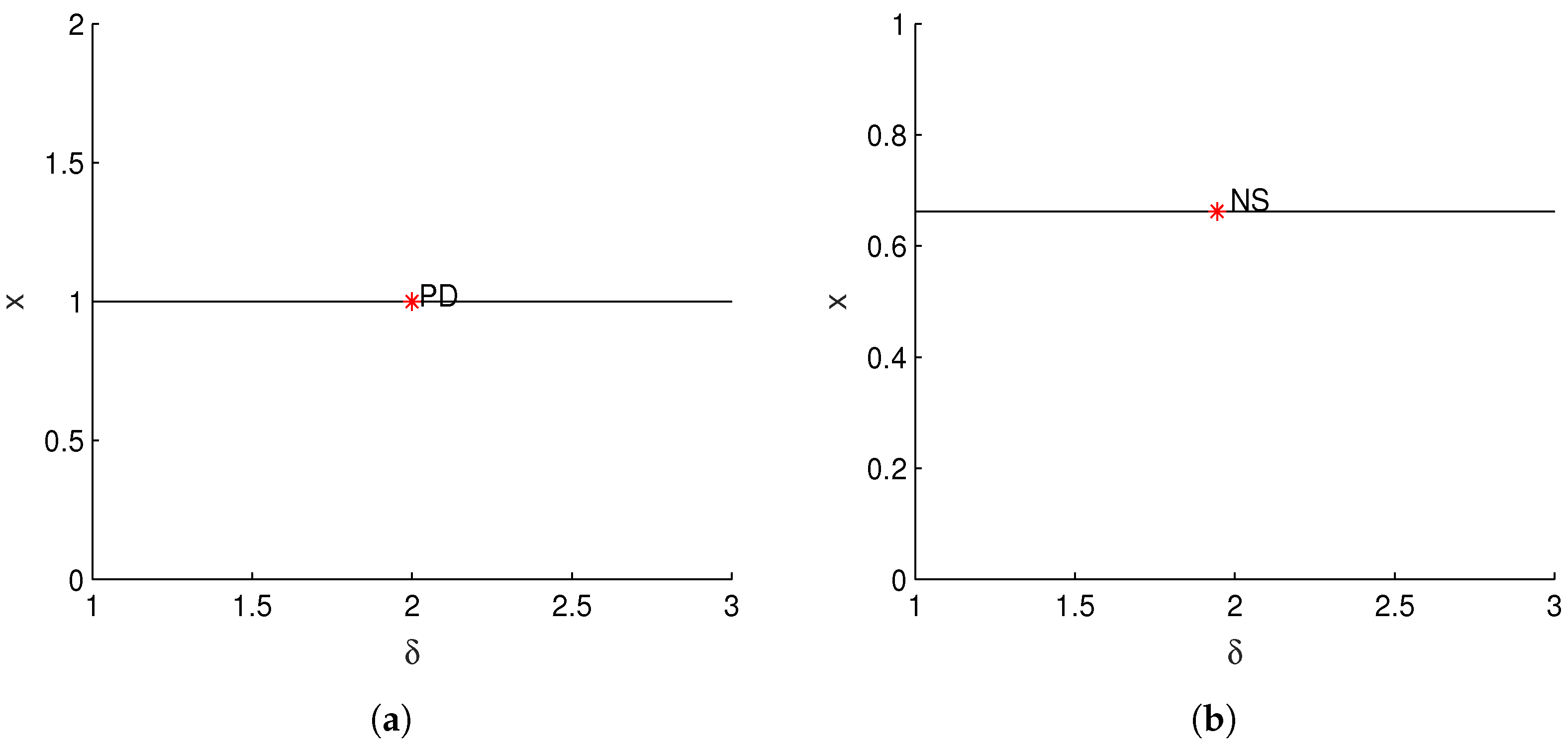
To validate the aforementioned results, we proceed with a numerical illustration. Fix $a=2.5,\alpha =0.75,\beta =4$, and treat $\delta$ as a free parameter. At $\delta =2$, $E_0$ experiences a flip bifurcation consistent with Theorem 1. This is captured in Figure 1a, which plots the continuation curve of $E_0$ and marks the critical point as PD. Moreover, a numerical continuation analysis is performed for $E_1$. With parameters $a=2.5,\alpha =0.75,\beta =0.5,\delta \in (1,3)$ and initial values $(0.662032,0.993048)$, model (3) is found to exhibit a Neimark–Sacker bifurcation at $\delta =1.94431$. Figure 1b depicts the continuation curve of $E_1$, highlighting the Neimark–Sacker bifurcation at the marked point NS.

4. Codimension-Two Bifurcation Analysis

Building on the prior analysis, this section consolidates the study of the codimension-two bifurcation for system (3) at $E_1$, adopting $\beta ,\delta$ as bifurcation variables.

4.1. Bifurcation Analysis of $E_1$ with 1:2 Resonance

We first discuss the 1:2 resonance bifurcation for system (3) near $E_1(x_1,y_1)$, focusing on the parameter changes in a small neighborhood of $F_{12}$.

Selecting arbitrary parameters $(a,\alpha ,\beta ,\delta )$ from $F_{12}$, the system (3) possesses exactly one positive equilibrium $E_1(x_1,y_1)$. Let $u=x-x_1,v=y-y_1$, and shift the equilibrium point $(x_1,y_1)$ to the origin point $(0,0)$; then, system (3) is transformed into a new form

$$\left[\begin{array}{c}u\\ v\end{array}\right]\to \left[\begin{array}{cc}1-\delta {\theta }_{11}& -\delta {\theta }_{12}\\ \delta {\theta }_{13}& 1+\delta {\theta }_{14}\end{array}\right]\left[\begin{array}{c}u\\ v\end{array}\right]+\left[\begin{array}{c}f(u,v)\\ g(u,v)\end{array}\right],$$

(6)

here

$$\begin{array}{ccc}& & f(u,v)={\displaystyle \frac{\delta y_1(a^2-6a{x}_1^2+x_1^4)}{{(x_1^2+a)}^4}}{u}^3+{\displaystyle \frac{\delta (6a{x}_1-2x_1^3)}{2{(x_1^2+a)}^3}}{u}^{2}v+\left[-\delta +{\displaystyle \frac{\delta y_1(6a{x}_1-2x_1^3)}{2{(x_1^2+a)}^3}}\right]u^2\hfill \\ & & +{\displaystyle \frac{\delta (x_1^2-a)}{{(x_1^2+a)}^2}}uv=a_{30}{u}^3+a_{21}{u}^{2}v+a_{20}{u}^2+a_{11}uv+O\left(\right(\left|u\right|+{\left|v\right|)}^4),\hfill \\ & & g(u,v)={\displaystyle \frac{\beta \delta (1-x_1)y_1^2}{x_1^4}}{u}^3-{\displaystyle \frac{2\beta \delta (1-x_1)y_1}{x_1^3}}{u}^{2}v+{\displaystyle \frac{\beta \delta (1-x_1)}{x_1^2}}u{v}^2\hfill \\ & & =b_{30}{u}^3+b_{21}{u}^{2}v+b_{12}u{v}^2+O\left(\right(\left|u\right|+{\left|v\right|)}^4).\hfill \end{array}$$

We denote

$$\mathit{J}(\overline{\beta },\overline{\delta })=\left[\begin{array}{cc}1-\delta {\theta }_{11}& -\delta {\theta }_{12}\\ \delta {\theta }_{13}& 1+\delta {\theta }_{14}\end{array}\right],$$

Consequently, there are $p_i,q_i\in {\mathbb{C}}^2$ satisfying the following relations:

$$\begin{array}{ccc}& & J{p}_1=-p_1,J{p}_2=-p_2+p_1,J^T{q}_2=-q_2,J^T{q}_1=-q_1+q_2,\hfill \\ & & <p_1,q_1>=<p_2,q_2>=1,<p_1,q_2>=<p_2,q_1>=0.\hfill \end{array}$$

Thus, we have

$$p_1(\tilde{\beta },\tilde{\delta })=\left[\begin{array}{c}{\displaystyle \frac{\delta {\theta }_{12}}{2-\delta {\theta }_{11}}}\\ 1\end{array}\right],p_2(\tilde{\beta },\tilde{\delta })=\left[\begin{array}{c}{\displaystyle \frac{\delta {\theta }_{12}}{{(2-\delta {\theta }_{11})}^2}}\\ 0\end{array}\right],$$

Consider the following transformation ${[u,v]}^T=p_1\overline{x}+p_2\overline{y}$. Now, in coordinates $(\overline{x},\overline{y})$, the model general representation of (6) is

$$\left[\begin{array}{c}\overline{x}\\ \overline{y}\end{array}\right]\to \left[\begin{array}{cc}-1+a_{10}(\overline{\beta },\overline{\delta })& 1+a_{01}(\overline{\beta },\overline{\delta })\\ b_{10}(\overline{\beta },\overline{\delta })& -1+b_{01}(\overline{\beta },\overline{\delta })\end{array}\right]\left[\begin{array}{c}\overline{x}\\ \overline{y}\end{array}\right]+\left[\begin{array}{c}\overline{f}(\overline{x},\overline{y})\\ \overline{g}(\overline{x},\overline{y})\end{array}\right],$$

(7)

where

$$\overline{f}(\overline{x},\overline{y})=\sum _{2\le j+k\le 3}{\overline{a}}_{jk}{\overline{x}}^j{\overline{y}}^k,\overline{g}(\overline{x},\overline{y})=\sum _{2\le j+k\le 3}{\overline{b}}_{jk}{\overline{x}}^j{\overline{y}}^k,$$

with

$$\begin{array}{ccc}& & a_{10}=2+\delta {\theta }_{14}+{\displaystyle \frac{{\delta }^2{\theta }_{12}{\theta }_{13}}{2-\delta {\theta }_{11}}},a_{01}=-1+{\displaystyle \frac{{\delta }^2{\theta }_{12}{\theta }_{13}}{{(2-\delta {\theta }_{11})}^2}},\hfill \\ & & b_{01}=2-\delta {\theta }_{11}-{\displaystyle \frac{{\delta }^2{\theta }_{12}{\theta }_{13}}{2-\delta {\theta }_{11}}},b_{10}=-{\delta }^2{\theta }_{12}{\theta }_{13}-(2-\delta {\theta }_{11})(2+\delta {\theta }_{14}),\hfill \\ & & {\overline{a}}_{12}={\displaystyle \frac{{\delta }^2{\theta }_{12}^2}{{(2-\delta {\theta }_{11})}^5}}\left[(2-\delta {\theta }_{11})b_{21}+3\delta {\theta }_{12}{b}_{30}\right],{\overline{a}}_{03}={\displaystyle \frac{{\delta }^3{\theta }_{12}^3}{{(2-\delta {\theta }_{11})}^6}}{b}_{30},\hfill \\ & & {\overline{a}}_{21}={\displaystyle \frac{\delta {\theta }_{12}}{{(2-\delta {\theta }_{11})}^4}}\left[{(2-\delta {\theta }_{11})}^2{b}_{12}+2\delta {\theta }_{12}(2-\delta {\theta }_{11})b_{21}+3{\delta }^2{\theta }_{12}^2{b}_{30}\right],\hfill \\ & & {\overline{a}}_{30}={\displaystyle \frac{\delta {\theta }_{12}}{{(2-\delta {\theta }_{11})}^3}}\left[{(2-\delta {\theta }_{11})}^2{b}_{12}+\delta {\theta }_{12}(2-\delta {\theta }_{11})b_{21}+{\delta }^2{\theta }_{12}^2{b}_{30}\right],\hfill \\ & & {\overline{b}}_{20}=\delta {\theta }_{12}{a}_{20}+(2-\delta {\theta }_{11})a_{11},{\overline{b}}_{11}=a_{11}+{\displaystyle \frac{2\delta {\theta }_{12}}{2-\delta {\theta }_{11}}}{a}_{20},\hfill \\ & & {\overline{b}}_{21}={\displaystyle \frac{3{\delta }^2{\theta }_{12}^2}{{(2-\delta {\theta }_{11})}^2}}{a}_{30}+{\displaystyle \frac{2\delta {\theta }_{12}}{2-\delta {\theta }_{11}}}{a}_{21}-(2-\delta {\theta }_{11}){\overline{a}}_{21},\hfill \\ & & {\overline{b}}_{12}={\displaystyle \frac{3{\delta }^2{\theta }_{12}^2}{{(2-\delta {\theta }_{11})}^3}}{a}_{30}+{\displaystyle \frac{\delta {\theta }_{12}}{{(2-\delta {\theta }_{11})}^2}}{a}_{21}-(2-\delta {\theta }_{11}){\overline{a}}_{12},\hfill \\ & & {\overline{b}}_{30}={\displaystyle \frac{{\delta }^2{\theta }_{12}^2}{2-\delta {\theta }_{11}}}{a}_{30}+\delta {\theta }_{12}{a}_{21}-(2-\delta {\theta }_{11}){\overline{a}}_{30},{\overline{b}}_{02}={\displaystyle \frac{\delta {\theta }_{12}}{{(2-\delta {\theta }_{11})}^2}}{a}_{20},\hfill \\ & & {\overline{b}}_{03}={\displaystyle \frac{{\delta }^2{\theta }_{12}^2}{{(2-\delta {\theta }_{11})}^4}}{a}_{30}-(2-\delta {\theta }_{11}){\overline{a}}_{03},{\overline{a}}_{20}={\overline{a}}_{11}={\overline{a}}_{02}=0.\hfill \end{array}$$

Implement the following invertible linear transformation

$$\left[\begin{array}{c}\overline{x}\\ \overline{y}\end{array}\right]\to \left[\begin{array}{cc}1+a_{01}(\overline{\beta },\overline{\delta })& 0\\ -a_{10}(\overline{\beta },\overline{\delta })& 1\end{array}\right]\left[\begin{array}{c}\tilde{x}\\ \tilde{y}\end{array}\right],$$

(8)

the mapping defined in (7) is reformulated as

$$\left[\begin{array}{c}\tilde{x}\\ \tilde{y}\end{array}\right]\to \left[\begin{array}{cc}-1& 1\\ c_1(\overline{\beta },\overline{\delta })& -1+c_2(\overline{\beta },\overline{\delta })\end{array}\right]\left[\begin{array}{c}\tilde{x}\\ \tilde{y}\end{array}\right]+\left[\begin{array}{c}G(\tilde{x},\tilde{y})\\ H(\tilde{x},\tilde{y})\end{array}\right],$$

(9)

where

$$\begin{array}{ccc}& & G(\tilde{x},\tilde{y})=\sum _{2\le j+k\le 3}{g}_{jk}{\tilde{x}}^j{\tilde{y}}^k,H(\tilde{x},\tilde{y})=\sum _{2\le j+k\le 3}{h}_{jk}{\tilde{x}}^j{\tilde{y}}^k,\hfill \\ & & c_1=b_{10}+a_{01}{b}_{10}-a_{10}{b}_{01},c_2=a_{10}+b_{01},\hfill \\ & & g_{20}=g_{02}=g_{11}=0,g_{12}={\overline{a}}_{12}-{\displaystyle \frac{3a_{10}}{1+a_{01}}}{\overline{a}}_{03},\hfill \\ & & g_{21}=(1+a_{01}){\overline{a}}_{21}-2a_{10}{\overline{a}}_{12}+{\displaystyle \frac{3a_{10}^2}{1+a_{01}}}{\overline{a}}_{03},g_{03}={\displaystyle \frac{1}{1+a_{01}}}{\overline{a}}_{03},\hfill \\ & & g_{30}=a_{10}^2{\overline{a}}_{12}-(1+a_{01})a_{10}{\overline{a}}_{21}+{(1+a_{01})}^2{\overline{a}}_{30}-{\displaystyle \frac{a_{10}^3}{1+a_{01}}}{\overline{a}}_{03},\hfill \\ & & h_{20}={(1+a_{01})}^2{\overline{b}}_{20}-a_{10}(1+a_{01}){\overline{b}}_{11}+a_{10}^2{\overline{b}}_{02},\hfill \\ & & h_{11}=(1+a_{01}){\overline{b}}_{11}-2a_{10}{\overline{b}}_{02},h_{02}={\overline{b}}_{02},\hfill \\ & & h_{21}={(1+a_{01})}^2{\overline{b}}_{21}-2a_{10}(1+a_{01}){\overline{b}}_{12}+3a_{10}^2{\overline{b}}_{03}+a_{10}{g}_{21},\hfill \\ & & h_{12}=(1+a_{01}){\overline{b}}_{12}-3a_{10}{\overline{b}}_{03}+a_{10}{g}_{12},h_{03}={\overline{b}}_{03},\hfill \\ & & h_{30}={(1+a_{01})}^3{\overline{b}}_{30}-a_{10}{(1+a_{01})}^2{\overline{b}}_{21}+a_{10}^2(1+a_{01}){\overline{b}}_{12}-a_{10}^3{\overline{b}}_{03}+a_{10}{g}_{30}.\hfill \end{array}$$

We employ the transformation

$$\begin{array}{c}\hfill \tilde{x}={\xi }_1+\sum _{2\le j+k\le 3}{\phi }_{jk}(\overline{\beta },\overline{\delta }){\xi }_1^j{\xi }_2^k,\tilde{y}={\xi }_2+\sum _{2\le j+k\le 3}{\psi }_{jk}(\overline{\beta },\overline{\delta }){\xi }_1^j{\xi }_2^k,\end{array}$$

where

$$\begin{array}{ccc}& & {\phi }_{20}={\displaystyle \frac{1}{4}}{h}_{20},{\phi }_{11}={\displaystyle \frac{1}{2}}{h}_{20}+{\displaystyle \frac{1}{4}}{h}_{11},{\phi }_{02}={\displaystyle \frac{1}{8}}{h}_{20}+{\displaystyle \frac{1}{4}}{h}_{11}+{\displaystyle \frac{1}{4}}{h}_{02},\hfill \\ & & {\phi }_{30}={\displaystyle \frac{1}{3}}{g}_{30}+{\displaystyle \frac{1}{9}}{h}_{30},{\phi }_{21}={\displaystyle \frac{1}{2}}{g}_{30}+{\displaystyle \frac{1}{2}}{g}_{21}+{\displaystyle \frac{5}{12}}{h}_{30}+{\displaystyle \frac{1}{4}}{h}_{21},\hfill \\ & & {\phi }_{12}={\displaystyle \frac{1}{6}}{g}_{30}+{\displaystyle \frac{1}{2}}{g}_{21}+g_{12}+{\displaystyle \frac{17}{36}}{h}_{30}+{\displaystyle \frac{3}{4}}{h}_{21}+h_{12},\hfill \\ & & {\psi }_{20}={\displaystyle \frac{1}{2}}{h}_{20},{\psi }_{11}={\displaystyle \frac{1}{2}}{h}_{20}+{\displaystyle \frac{1}{2}}{h}_{11},{\psi }_{02}={\displaystyle \frac{1}{4}}{h}_{11}+{\displaystyle \frac{1}{2}}{h}_{02},\hfill \\ & & {\psi }_{30}={\displaystyle \frac{1}{3}}{h}_{30},{\psi }_{21}={\displaystyle \frac{1}{2}}{h}_{30}+{\displaystyle \frac{1}{2}}{h}_{21},{\psi }_{12}={\displaystyle \frac{1}{6}}{h}_{30}+{\displaystyle \frac{1}{2}}{h}_{21}+h_{12}.\hfill \end{array}$$

The normal form for the 1:2 resonance is therefore obtained as shown below:

$$\left[\begin{array}{c}{\xi }_1\\ {\xi }_2\end{array}\right]\to \left[\begin{array}{cc}-1& 1\\ c_1(\overline{\beta },\overline{\delta })& -1+c_2(\overline{\beta },\overline{\delta })\end{array}\right]\left[\begin{array}{c}{\xi }_1\\ {\xi }_2\end{array}\right]+\left[\begin{array}{c}0\\ C(\overline{\beta },\overline{\delta }){\xi }_1^3+D(\overline{\beta },\overline{\delta }){\xi }_1^2{\xi }_2\end{array}\right],$$

(10)

where

$$\begin{array}{ccc}& & C(\overline{\beta },\overline{\delta })=h_{30}+{\displaystyle \frac{1}{2}}{h}_{20}^2+{\displaystyle \frac{1}{2}}{h}_{20}{h}_{11},\hfill \\ & & D(\overline{\beta },\overline{\delta })=h_{21}+3g_{30}+{\displaystyle \frac{5}{4}}{h}_{20}{h}_{11}+h_{20}{h}_{02}+h_{20}^2+{\displaystyle \frac{1}{2}}{h}_{11}^2.\hfill \end{array}$$

Combining Lemma 9.10 and Theorem 9.3 in [23], the smooth equivalence of map (10) to the system is established.

$$\left[\begin{array}{c}\dot{{\tau }_1}\\ \dot{{\tau }_2}\end{array}\right]\to \left[\begin{array}{cc}0& 1\\ r_1\left(\theta \right)& r_2\left(\theta \right)\end{array}\right]\left[\begin{array}{c}{\tau }_1\\ {\tau }_2\end{array}\right]+\left[\begin{array}{c}0\\ C_1\left(\theta \right){\tau }_1^3+D_1\left(\theta \right){\tau }_1^2{\tau }_2\end{array}\right],$$

(11)

where

$$\left\{\begin{array}{c}{r}_1\left(\theta \right)=4{\theta }_1+{O\left(\right|\left|\theta \right||}^2),\hfill \\ r_2\left(\theta \right)=-2{\theta }_1-2{\theta }_2+{O\left(\right|\left|\theta \right||}^2),\hfill \end{array}\right.$$

and

$$\theta ={({\theta }_1,{\theta }_2)}^T,C_1\left(0\right)=4C\left(0\right),D_1\left(0\right)=-2D\left(0\right)-6C\left(0\right).$$

For the approximating system (11), we now analyze its bifurcations under the nondegeneracy conditions: $C_1\left(0\right)\ne 0,D_1\left(0\right)\ne 0$.

Without loss of generality, assume that $C_1\left(0\right)>0,D_1\left(0\right)<0$ (reversing time if necessary); we rescale the variables, parameters, and time in (11) to derive the system

$$\left\{\begin{array}{c}\dot{l_1}=l_2,\hfill \\ \dot{l_2}=k_1{l}_1+k_2{l}_2+l_1^3-l_1^2{l}_2,\hfill \end{array}\right.$$

(12)

where $k_1={\displaystyle \frac{D_1^2\left(\theta \right)}{C_1^2\left(\theta \right)}}{r}_1\left(\theta \right),k_2=-{\displaystyle \frac{D_1\left(\theta \right)}{C_1\left(\theta \right)}}{r}_2\left(\theta \right)$. For system (12), there exists a pitchfork bifurcation curve $F=\{(k_1,k_2):k_1=0\}$ leading to the emergence of two symmetrically coupled saddles. It is not difficult to obtain $r_1=0,i.e.{\theta }_1=0$ for $k_1=0$. With analogous argument, we can obtain the nondegenerate Neimark–Sacker bifurcation condition $H=\{(k_1,k_2):k_2=0,k_1<0\}$.

Similarly, crossing the curve

$$CH=\{(k_1,k_2):k_2=-{\displaystyle \frac{1}{5}}{k}_1+O\left(k_1\right),k_1<0\},$$

the cycle is eliminated via a heteroclinic bifurcation.

Combining the preceding analysis with findings from [23,24,25,26], the subsequent results are derived.

Theorem 2.

If $C(\overline{\beta },\overline{\delta })\ne 0$ and $D(\overline{\beta },\overline{\delta })+3C(\overline{\beta },\overline{\delta })\ne 0,$ then the map (3) exhibits the following bifurcation behaviors:

(I) 

When $C(\overline{\beta },\overline{\delta })<0,$ the critical point is classified as a saddle; whereas if $C(\overline{\beta },\overline{\delta })>0,$ it is identified as an elliptic point. The condition $D(\overline{\beta },\overline{\delta })+3C(\overline{\beta },\overline{\delta })\ne 0$ determines the bifurcation scenario near the 1:2 point.

(II) 

A flip bifurcation curve similar to the pitchfork bifurcation curve $F=\{(k_1,k_2):k_1=0\}$ exists. A stable double-period cycle splits from $E_1$ when crossing the curve.

(III) 

A stable closed invariant cycle is observed to bifurcate from $E_1$ when traversing the Neimark–Sacker bifurcation curve $H=\{(k_1,k_2):k_2=0,k_1<0\}$.

(IV) 

A heteroclinic bifurcation curve $CH=\{(k_1,k_2):k_2=-{\displaystyle \frac{1}{5}}{k}_1+O\left(k_1\right),k_1<0\}$ exists. This implies that long-period cycles emerge and vanish through fold bifurcations within an exponentially narrow interval near the critical point $CH$.

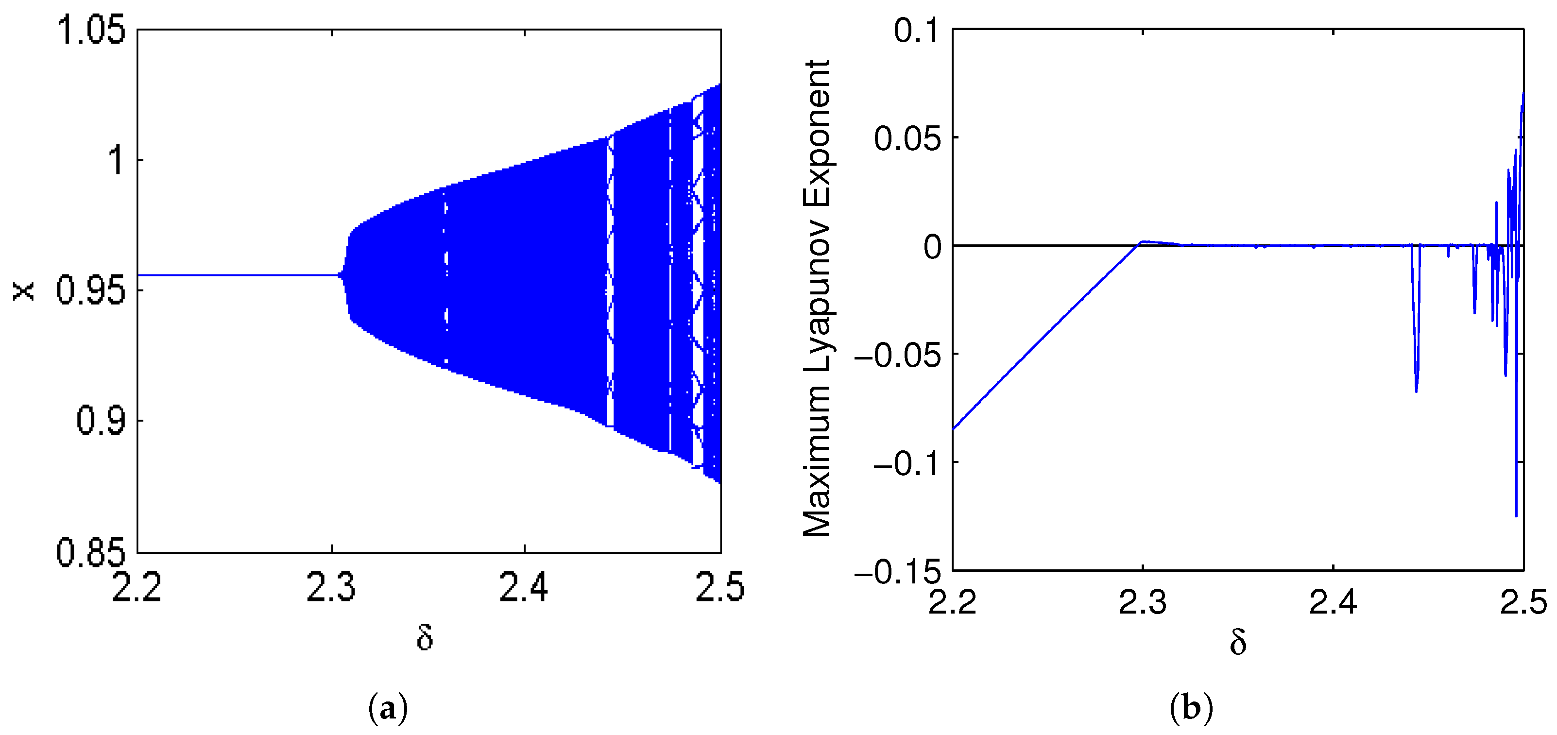
Example 1.

The unique fixed point $E_1(0.95578,0.150944)$ is observed at $\delta =2.378$ when δ is swept through $[2.2,2.5]$ in map (3), with $a=2.5,\alpha =0.75,\beta =4.749$. Further calculations yield eigenvalues ${\lambda }_{1,2}=-1$ for the Jacobian matrix $J\left(E_1\right)$, along with $C(\overline{\beta },\overline{\delta })=19.2162,D(\overline{\beta },\overline{\delta })=-1.3147$. Theorem 2 confirms that system (3) undergoes a 1:2 resonance bifurcation at $E_1$ under these conditions.

Figure 2 presents the codimension-two bifurcation diagrams exhibiting a prominent 1:2 resonance dynamics. Figure 2a illustrates the two-dimensional bifurcation diagram for map (3) in the $(\delta ,x)$ plane at $\overline{\beta }=4.749$, with $\delta$ ranging from $2.2$ to $2.5$, which is a neighborhood around $\overline{\delta }$. The robust Lyapunov exponent test in Figure 2b validates the presence of periodic orbits and chaotic behaviors. 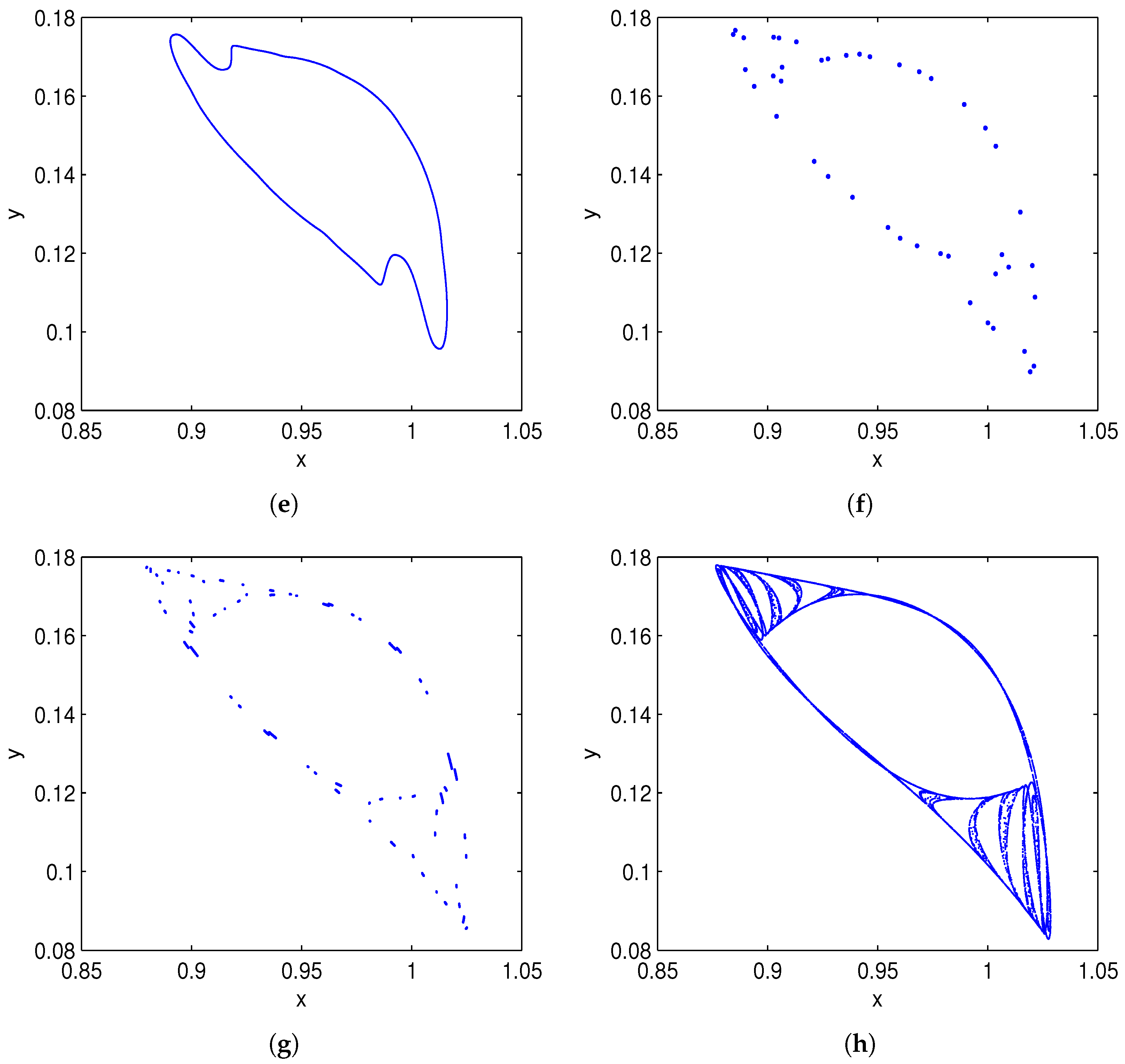In Figure 2b, negative Lyapunov exponents reflect the existence of stable fixed points or periodic windows, whereas positive exponents highlight chaotic regions. The corresponding phase portraits are displayed in Figure 3 for different $\delta$ near $\overline{\delta }=2.378$. An invariant curve bifurcates from $E_1$ due to a Neimark–Sacker bifurcation at $\overline{\delta }=2.378,\overline{\beta }=4.749$. After that point, quasi-periodic motion appears in the system, and chaotic motion finally occurs, as shown in Figure 3h.

4.2. Bifurcation Analysis of $E_1$ with 1:3 Resonance

This subsection addresses codimension-two bifurcation with 1:3 resonance in model (3). Firstly, we translate $E_1$ to the origin and expand the system into a Taylor series (analogous to system (6)). Subsequently, the Jacobian matrix at $E_1$ is derived as

$$\mathit{J}(\tilde{\beta },\tilde{\delta })=\left[\begin{array}{cc}1-\delta {\theta }_{11}& -\delta {\theta }_{12}\\ \delta {\theta }_{13}& 1+\delta {\theta }_{14}\end{array}\right].$$

The corresponding eigenvalues are ${\lambda }_{1,2}={\displaystyle \frac{-1\pm \sqrt{3}i}{2}}.$ The eigenvalues $q_3(\tilde{\beta },\tilde{\delta })\in {\mathbb{C}}^2$ and the adjoint eigenvector $p_3(\tilde{\beta },\tilde{\delta })\in {\mathbb{C}}^2$ are straightforward to obtain, as they naturally satisfy the required conditions.

$$J{q}_3={\displaystyle \frac{\sqrt{3}i-1}{2}}{q}_3,J^T{p}_3=-{\displaystyle \frac{\sqrt{3}i+1}{2}}{p}_3,<p_3,q_3>=1,$$

Hence, we obtain

$$q_3(\tilde{\beta },\tilde{\delta })=\left[\begin{array}{c}\delta {\theta }_{12}\\ {\displaystyle \frac{3-\sqrt{3}i}{2}}-\delta {\theta }_{11}\end{array}\right],p_3(\tilde{\beta },\tilde{\delta })=\left[\begin{array}{c}{\displaystyle \frac{3-\sqrt{3}i(3+2\delta {\theta }_{14})}{6\delta {\theta }_{12}}}\\ -{\displaystyle \frac{\sqrt{3}i}{3}}\end{array}\right].$$

For any $Z={(u,v)}^{\mathit{T}}\in {\mathbb{R}}^2$, the representation $Z=z{q}_3+\overline{z}\overline{q_3}$ holds, enabling system (6) to be reformulated as

$$\left[\begin{array}{c}z\\ \overline{z}\end{array}\right]\to \left[\begin{array}{cc}{\displaystyle \frac{\sqrt{3}i-1}{2}}& 0\\ 0& {\displaystyle \frac{-\sqrt{3}i-1}{2}}\end{array}\right]\left[\begin{array}{c}z\\ \overline{z}\end{array}\right]+\left[\begin{array}{c}{\displaystyle \sum _{2\le j+k\le 3}}{\displaystyle \frac{g_{jk}}{j!k!}}{z}^j{\overline{z}}^k\\ {\displaystyle \sum _{2\le j+k\le 3}}{\displaystyle \frac{{\overline{g}}_{jk}}{j!k!}}{z}^j{\overline{z}}^k\end{array}\right],$$

(13)

where

$$\begin{array}{ccc}& & g_{20}=2{\delta }^2{\theta }_{12}^2\left[\left({\displaystyle \frac{3-\sqrt{3}i}{2}}-\delta {\theta }_{11}\right)a_{11}+\delta {\theta }_{12}{a}_{20}\right],\hfill \\ & & g_{02}=2{\delta }^2{\theta }_{12}^2\left[\left({\displaystyle \frac{3+\sqrt{3}i}{2}}-\delta {\theta }_{11}\right)a_{11}+\delta {\theta }_{12}{a}_{20}\right],\hfill \\ & & g_{11}=2{\delta }^2{\theta }_{12}^2\left({\displaystyle \frac{3-2\delta {\theta }_{11}}{2}}{a}_{11}+\delta {\theta }_{12}{a}_{20}\right),\hfill \\ & & g_{21}=2{\delta }^2{\theta }_{12}^2\left({\displaystyle \frac{3+\sqrt{3}i}{2}}-\delta {\theta }_{11}\right)\left[\left({\displaystyle \frac{9-\sqrt{3}i}{2}}-3\delta {\theta }_{11}\right)b_{21}+3\delta {\theta }_{12}{b}_{30}\right]\hfill \\ & & +2\delta {\theta }_{12}{b}_{12}\left({\displaystyle \frac{3-\sqrt{3}i}{2}}-\delta {\theta }_{11}\right)\left({\displaystyle \frac{3+\sqrt{3}i}{2}}-\delta {\theta }_{11}\right)\left({\displaystyle \frac{9+\sqrt{3}i}{2}}-3\delta {\theta }_{11}\right)\hfill \\ & & +2{\delta }^3{\theta }_{12}^3\left[\left({\displaystyle \frac{9-\sqrt{3}i}{2}}-3\delta {\theta }_{11}\right)a_{21}+3\delta {\theta }_{12}{a}_{30}\right],\hfill \\ & & g_{12}=2{\delta }^2{\theta }_{12}^2\left({\displaystyle \frac{3+\sqrt{3}i}{2}}-\delta {\theta }_{11}\right)\left[\left({\displaystyle \frac{9+\sqrt{3}i}{2}}-3\delta {\theta }_{11}\right)b_{21}+3\delta {\theta }_{12}{b}_{30}\right]\hfill \\ & & +2\delta {\theta }_{12}{b}_{12}{\left({\displaystyle \frac{3+\sqrt{3}i}{2}}-\delta {\theta }_{11}\right)}^2\left({\displaystyle \frac{9-\sqrt{3}i}{2}}-3\delta {\theta }_{11}\right)\hfill \\ & & +2{\delta }^3{\theta }_{12}^3\left[\left({\displaystyle \frac{9+\sqrt{3}i}{2}}-3\delta {\theta }_{11}\right)a_{21}+3\delta {\theta }_{12}{a}_{30}\right],\hfill \\ & & g_{30}=6\delta {\theta }_{12}\left({\displaystyle \frac{3+\sqrt{3}i}{2}}-\delta {\theta }_{11}\right)\left[\delta {\theta }_{12}{b}_{21}\left({\displaystyle \frac{3-\sqrt{3}i}{2}}-\delta {\theta }_{11}\right)+{\left({\displaystyle \frac{3-\sqrt{3}i}{2}}-\delta {\theta }_{11}\right)}^2{b}_{12}+{\delta }^2{\theta }_{12}^2{b}_{30}\right]\hfill \\ & & +6{\delta }^3{\theta }_{12}^3\left[\left({\displaystyle \frac{3-\sqrt{3}i}{2}}-\delta {\theta }_{11}\right)a_{21}+\delta {\theta }_{12}{a}_{30}\right],\hfill \\ & & g_{03}=6\delta {\theta }_{12}\left({\displaystyle \frac{3+\sqrt{3}i}{2}}-\delta {\theta }_{11}\right)\left[\delta {\theta }_{12}{b}_{21}\left({\displaystyle \frac{3+\sqrt{3}i}{2}}-\delta {\theta }_{11}\right)+{\left({\displaystyle \frac{3+\sqrt{3}i}{2}}-\delta {\theta }_{11}\right)}^2{b}_{12}+{\delta }^2{\theta }_{12}^2{b}_{30}\right]\hfill \\ & & +6{\delta }^3{\theta }_{12}^3\left[\left({\displaystyle \frac{3+\sqrt{3}i}{2}}-\delta {\theta }_{11}\right)a_{21}+\delta {\theta }_{12}{a}_{30}\right].\hfill \end{array}$$

Here, ${\overline{g}}_{ij}$ and $g_{ij}$ are complex conjugates of each other.

Hence, the analysis can be simplified to studying

$$z\to {\displaystyle \frac{\sqrt{3}i-1}{2}}z+\sum _{2\le j+k\le 3}{\displaystyle \frac{g_{jk}}{j!k!}}{z}^j{\overline{z}}^k,$$

(14)

given that the second component of (13) represents the complex conjugate of the first.

To eliminate some second-order terms, a transformation is introduced

$$z=w+{\displaystyle \frac{1}{2}}{h}_{20}{w}^2+h_{11}w\overline{w}+{\displaystyle \frac{1}{2}}{h}_{02}{\overline{w}}^2,$$

(15)

where $h_{jk}$ with $j+k=2$ will be given later. Utilizing transformation (15) along with its inverse transformation, (14) becomes

$$w\to {\displaystyle \frac{\sqrt{3}i-1}{2}}w+\sum _{2\le j+k\le 3}{\displaystyle \frac{{\sigma }_{jk}}{j!k!}}{w}^j{\overline{w}}^k,$$

(16)

where

$$\begin{array}{ccc}& & {\sigma }_{20}={\lambda }_1{h}_{20}+g_{20}-{\lambda }_1^2{h}_{20},{\sigma }_{11}={\lambda }_1{h}_{11}+g_{11}-{\left|{\lambda }_1\right|}^2{h}_{11},\hfill \\ & & {\sigma }_{30}=3(1-{\lambda }_1)g_{20}{h}_{20}+3g_{11}{\overline{h}}_{02}+g_{30}+3({\lambda }_1^3-{\lambda }_1^2)h_{20}^2+3({\lambda }_1^3-|{\lambda }_1{|}^2)h_{11}{\overline{h}}_{02}\hfill \\ & & -3{\lambda }_1{\overline{g}}_{02}{h}_{11},{\sigma }_{02}={\lambda }_1{h}_{02}+g_{02}-{\overline{\lambda }}_1^2{h}_{02},\hfill \\ & & {\sigma }_{21}=2g_{11}{\overline{h}}_{11}+g_{11}{h}_{20}+2g_{20}{h}_{11}+g_{02}{\overline{h}}_{02}+g_{21}+2{\lambda }_1^2({\overline{\lambda }}_1-1)h_{20}{h}_{11}-2{\lambda }_1{g}_{11}{h}_{20}\hfill \\ & & -{\overline{\lambda }}_1{g}_{20}{h}_{11}+2|{\lambda }_1{|}^2({\lambda }_1-1)|h_{11}{|}^2-2{\lambda }_1{h}_{11}{\overline{g}}_{11}+{\left|{\lambda }_1\right|}^2({\lambda }_1-1)h_{11}{h}_{20}\hfill \\ & & -{\overline{\lambda }}_1{\overline{g}}_{02}{h}_{02}+{\overline{\lambda }}_1({\lambda }_1^2-{\overline{\lambda }}_1){\left|h_{02}\right|}^2,\hfill \\ & & {\sigma }_{12}=2g_{11}{h}_{11}+g_{11}{\overline{h}}_{20}+2g_{02}{\overline{h}}_{11}+g_{20}{h}_{02}+g_{12}+{\lambda }_1({\overline{\lambda }}_1^2-{\lambda }_1)h_{20}{h}_{02}-{\lambda }_1{\overline{g}}_{20}{h}_{11}\hfill \\ & & -2{\lambda }_1{g}_{02}{h}_{20}-2{\overline{\lambda }}_1{g}_{11}{h}_{11}+2|{\lambda }_1{|}^2(\overline{{\lambda }_1}-1)h_{11}^2+{\left|{\lambda }_1\right|}^2({\overline{\lambda }}_1-1)h_{11}{\overline{h}}_{20}\hfill \\ & & +2{\overline{\lambda }}_1^2({\lambda }_1-1)h_{02}{\overline{h}}_{11}-2{\overline{\lambda }}_1{\overline{g}}_{11}{h}_{02},\hfill \\ & & {\sigma }_{03}=3g_{11}{h}_{02}+3g_{02}{\overline{h}}_{20}+g_{03}+3({\overline{\lambda }}_1^3-|{\lambda }_1{|}^2)h_{11}{h}_{02}-3{\overline{\lambda }}_1{g}_{02}{h}_{11}-3{\overline{\lambda }}_1{\overline{g}}_{20}{h}_{02}\hfill \\ & & +3{\overline{\lambda }}_1^2({\overline{\lambda }}_1-1)h_{02}{\overline{h}}_{20},{\lambda }_1={\displaystyle \frac{\sqrt{3}i-1}{2}}.\hfill \end{array}$$

Now, it should be noted that the quadratic terms of (16) should vanish if

$$h_{20}={\displaystyle \frac{\sqrt{3}i}{3}}{g}_{20},h_{11}={\displaystyle \frac{3+\sqrt{3}i}{6}}{g}_{11},h_{02}=0.$$

Furthermore, the following transformation annihilates some cubic terms:

$$w=\xi +{\displaystyle \frac{1}{6}}{h}_{30}{\xi }^3+{\displaystyle \frac{1}{2}}{h}_{12}\xi {\overline{\xi }}^2+{\displaystyle \frac{1}{2}}{h}_{21}{\xi }^2\overline{\xi }+{\displaystyle \frac{1}{6}}{h}_{03}{\overline{\xi }}^3.$$

(17)

Model (16) is reformulated via (17), and its inverse transformation is defined as

$$\begin{array}{c}\hfill \xi \to {\displaystyle \frac{\sqrt{3}i-1}{2}}\xi +{\displaystyle \frac{1}{2}}{g}_{02}{\overline{\xi }}^2+\sum _{2\le j+k\le 3}{\displaystyle \frac{r_{jk}}{j!k!}}{\xi }^j{\overline{\xi }}^k,\end{array}$$

where

$$\begin{array}{ccc}& & r_{30}={\displaystyle \frac{\sqrt{3}i-3}{2}}{h}_{30}+{\sigma }_{30},r_{21}={\sigma }_{21},\hfill \\ & & r_{12}=\sqrt{3}i{h}_{12}+{\sigma }_{12},r_{03}={\displaystyle \frac{\sqrt{3}i-3}{2}}{h}_{03}+{\sigma }_{03},\hfill \end{array}$$

upon setting

$$h_{30}={\displaystyle \frac{3+\sqrt{3}i}{6}}{\sigma }_{30},h_{12}={\displaystyle \frac{\sqrt{3}i}{3}}{\sigma }_{12},h_{03}={\displaystyle \frac{3+\sqrt{3}i}{6}}{\sigma }_{03},h_{21}=0.$$

Therefore, the desired normal form of 1:3 resonance bifurcation is derived as

$$\xi \to {\displaystyle \frac{\sqrt{3}i-1}{2}}\xi +C(\tilde{\beta },\tilde{\delta }){\overline{\xi }}^2+D(\tilde{\beta },\tilde{\delta }){\xi \left|\xi \right|}^2+{O\left(\right|\xi |}^4),$$

(18)

where

$$\begin{array}{ccc}& & C(\tilde{\beta },\tilde{\delta })={\displaystyle \frac{1}{2}}{g}_{02},\hfill \\ & & D(\tilde{\beta },\tilde{\delta })={\displaystyle \frac{3+\sqrt{3}i}{6}}{g}_{20}{g}_{11}+{\displaystyle \frac{3-\sqrt{3}i}{6}}{\left|g_{11}\right|}^2+{\displaystyle \frac{1}{2}}{g}_{21}.\hfill \end{array}$$

Let

$$\begin{array}{ccc}& & C_1(\tilde{\beta },\tilde{\delta })=3\overline{{\lambda }_1}C(\tilde{\beta },\tilde{\delta })=-{\displaystyle \frac{3}{2}}(\sqrt{3}i+1)C(\tilde{\beta },\tilde{\delta }),\hfill \\ & & D_1(\tilde{\beta },\tilde{\delta })=-3|C(\tilde{\beta },\tilde{\delta }){|}^2+3{\lambda }_1^{2}D(\tilde{\beta },\tilde{\delta })=-3{\left|C(\tilde{\beta },\tilde{\delta })\right|}^2-{\displaystyle \frac{3}{2}}(\sqrt{3}i+1)D(\tilde{\beta },\tilde{\delta }).\hfill \end{array}$$

Thus, the bifurcation curves in model (18) can be locally characterized near the origin.

Theorem 3.

If $(\tilde{\beta },\tilde{\delta })\in F_{13}$, $C_1(\tilde{\beta },\tilde{\delta })\ne 0$, and $Re{D}_1(\tilde{\beta },\tilde{\delta })\ne 0$, the model (3) then exhibits the following dynamic characteristics at point $E_1$:

(I) 

Under the conditions $C_1(\tilde{\beta },\tilde{\delta })\ne 0$ and $Re{D}_1(\tilde{\beta },\tilde{\delta })\ne 0$, a 1:3 resonance bifurcation occurs at $E_1$. The stability of the closed invariant curve near the 1:3 resonance point depends on the sign of $Re{D}_1(\tilde{\beta },\tilde{\delta })$: it is stable for $Re{D}_1<0$ and unstable for $Re{D}_1>0$.

(II) 

At the trivial fixed point $E_0$, a nondegenerate Neimark–Sacker bifurcation takes place.

(III) 

A period-three saddle cycle arises in model (18), which is associated with the saddle points $E_k(k=1,2,3)$.

(IV) 

The stable and unstable invariant manifolds of the period-three cycle in model (18) form a homoclinic structure through transverse intersection in an exponentially small parameter region.

Example 2.

Let $a=2.5,\alpha =0.75$. We can obtain the critical parameter values $\tilde{\delta }=2.037$ and $\tilde{\beta }=0.794$, and J has two eigenvalues ${\lambda }_{1,2}={\displaystyle \frac{-1\pm \sqrt{3}i}{2}}.$ Then, a unique fixed point $E_1(0.803428,0.758906)$ exists in model (3), and $C(\tilde{\beta },\tilde{\delta })=-0.4316-0.0836i,D(\tilde{\beta },\tilde{\delta })=-0.2598+0.0964i$. A 1:3 resonance bifurcation occurs at $E_1$ in model (3), as indicated by Theorem 3.

Figure 4 presents the two-dimensional bifurcation diagrams exhibiting a 1:3 strong resonance in both the $(\delta ,x)$ and $(\delta ,y)$ space when $\tilde{\beta }=0.794$, with $\delta$ varying within a neighborhood around $\tilde{\delta }=2.037$. Figure 4b displays the corresponding Maximum Lyapunov Exponents (MLEs) related to Figure 4a. It is evident that some MLE values are negative, indicating that system (3) is stable in the vicinity of the 1:3 resonance point $E_1$. 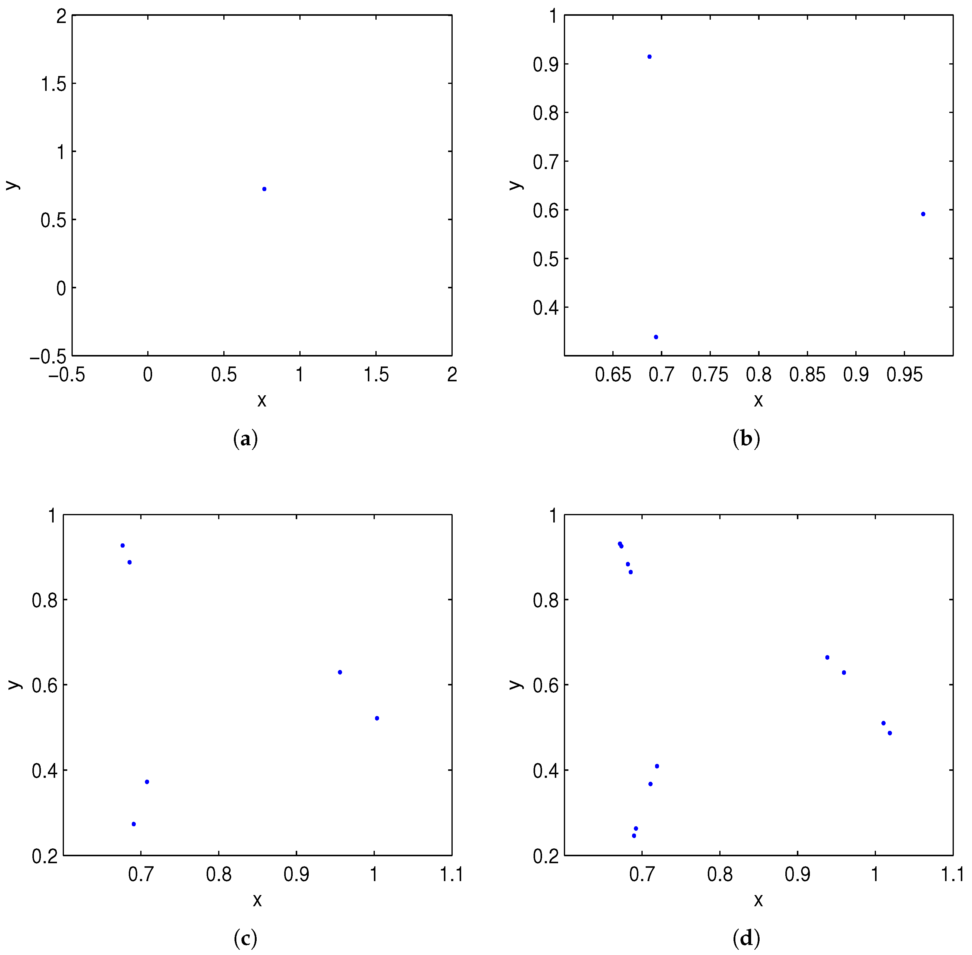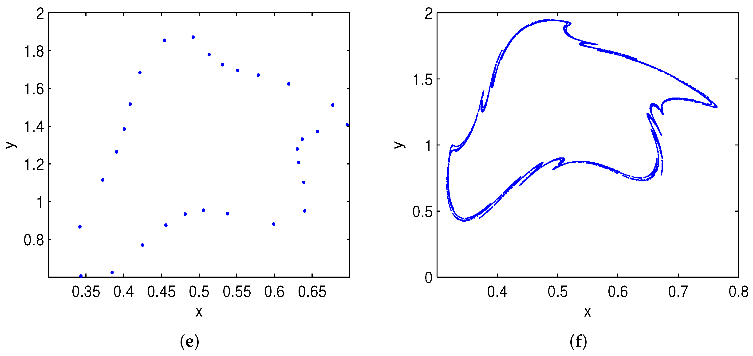Figure 5 presents the corresponding phase portraits for different $\delta$ values in a neighborhood around $\delta =2.037$. Periodic orbits of periods 1, 3, 6, 12, 24, and multi-periodic orbits (shown in Figure 5g) can also be observed, eventually leading to chaotic behavior (shown in Figure 5h). This follows the classical route to chaos.

4.3. Bifurcation Analysis of $E_1$ with 1:4 Resonance

At last, we investigate the 1:4 resonance behavior in system (3) by randomly choosing the values $(a,\alpha ,\beta ,\delta )$ from bifurcation set $F_{14}$. By translating $E_1$ to the origin, we can express the model as a Taylor series expansion, which is similar to system (6). The corresponding Jacobian matrix at $E_1$ is calculated as below as

$$\mathit{J}(\widehat{\beta },\widehat{\delta })=\left[\begin{array}{cc}1-\delta {\theta }_{11}& -\delta {\theta }_{12}\\ \delta {\theta }_{13}& 1+\delta {\theta }_{14}\end{array}\right].$$

$\mathit{J}$ has two eigenvalues ${\lambda }_{1,2}=\pm i$. A pair of adjoint eigenvectors $q_4(\widehat{\beta },\widehat{\delta })\in {\mathbb{C}}^2,p_4(\widehat{\beta },\widehat{\delta })\in {\mathbb{C}}^2$ satisfying the following conditions can be easily identified.

$$J{q}_4=i{q}_4,J^T{p}_4=-i{p}_4,<p_4,q_4>=1.$$

Hence, we obtain

$$q_4(\widehat{\beta },\widehat{\delta })=\left[\begin{array}{c}\delta {\theta }_{12}\\ 1-\delta {\theta }_{11}-i\end{array}\right],p_4(\widehat{\beta },\widehat{\delta })=\left[\begin{array}{c}{\displaystyle \frac{1-i(1+\delta {\theta }_{14})}{2\delta {\theta }_{12}}}\\ -{\displaystyle \frac{i}{2}}\end{array}\right].$$

To represent any vector $Z={(u,v)}^{\mathit{T}}\in {\mathbb{R}}^2$ in the form $Z=z{q}_4+\overline{z}\overline{q_4}$, we can translate the system (6) into

$$z\to iz+\sum _{2\le j+k\le 3}{\displaystyle \frac{g_{jk}}{j!k!}}{z}^j{\overline{z}}^k,$$

(19)

where

$$\begin{array}{ccc}& & g_{20}=2{\delta }^2{\theta }_{12}^2\left[\left(1-\delta {\theta }_{11}-i\right)a_{11}+\delta {\theta }_{12}{a}_{20}\right],\hfill \\ & & g_{02}=2{\delta }^2{\theta }_{12}^2\left[\left(1-\delta {\theta }_{11}+i\right)a_{11}+\delta {\theta }_{12}{a}_{20}\right],\hfill \\ & & g_{11}=2{\delta }^2{\theta }_{12}^2\left[(1-\delta {\theta }_{11})a_{11}+\delta {\theta }_{12}{a}_{20}\right],\hfill \\ & & g_{21}=2{\delta }^2{\theta }_{12}^2\left(1-\delta {\theta }_{11}+i\right)\left[\left(3-3\delta {\theta }_{11}-i\right)b_{21}+3\delta {\theta }_{12}{b}_{30}\right]+2{\delta }^3{\theta }_{12}^3\left[\left(3-3\delta {\theta }_{11}-i\right)a_{21}+3\delta {\theta }_{12}{a}_{30}\right]\hfill \\ & & +2\delta {\theta }_{12}{b}_{12}\left(1-\delta {\theta }_{11}-i\right)\left(1-\delta {\theta }_{11}+i\right)\left(3-3\delta {\theta }_{11}+i\right),\hfill \\ & & g_{12}=2{\delta }^2{\theta }_{12}^2\left(1-\delta {\theta }_{11}+i\right)\left[\left(3-3\delta {\theta }_{11}+i\right)b_{21}+3\delta {\theta }_{12}{b}_{30}\right]+2{\delta }^3{\theta }_{12}^3\left[\left(3-3\delta {\theta }_{11}+i\right)a_{21}+3\delta {\theta }_{12}{a}_{30}\right]\hfill \\ & & +2\delta {\theta }_{12}{b}_{12}{\left(1-\delta {\theta }_{11}-i\right)}^2\left(3-3\delta {\theta }_{11}-i\right),\hfill \\ & & g_{30}=6\delta {\theta }_{12}\left(1-\delta {\theta }_{11}-i\right)\left[\left(1-\delta {\theta }_{11}-i\right)\delta {\theta }_{12}{b}_{21}+{\left(1-\delta {\theta }_{11}-i\right)}^2{b}_{12}+{\delta }^2{\theta }_{12}^2{b}_{30}\right]\hfill \\ & & +6{\delta }^3{\theta }_{12}^3\left[\left(1-\delta {\theta }_{11}-i\right)a_{21}+\delta {\theta }_{12}{a}_{30}\right],\hfill \\ & & g_{03}=6\delta {\theta }_{12}\left(1-\delta {\theta }_{11}+i\right)\left[\left(1-\delta {\theta }_{11}+i\right)\delta {\theta }_{12}{b}_{21}+{\left(1-\delta {\theta }_{11}+i\right)}^2{b}_{12}+{\delta }^2{\theta }_{12}^2{b}_{30}\right]\hfill \\ & & +6{\delta }^3{\theta }_{12}^3\left[\left(1-\delta {\theta }_{11}+i\right)a_{21}+\delta {\theta }_{12}{a}_{30}\right].\hfill \end{array}$$

Now the transformation, which is depicted in (15) along with its inverse transformation, is utilized to eliminate the quadratic terms from (19); then, it becomes

$$w\to iw+\sum _{2\le j+k\le 3}{\displaystyle \frac{{\sigma }_{jk}}{j!k!}}{w}^j{\overline{w}}^k,$$

(20)

where ${\sigma }_{jk}$ is determined by

$$\begin{array}{ccc}& & {\sigma }_{20}=i{h}_{20}+g_{20}+h_{20},{\sigma }_{11}=i{h}_{11}+g_{11}-h_{11},{\sigma }_{02}=i{h}_{02}+g_{02}+h_{02},\hfill \\ & & {\sigma }_{21}=2g_{11}{\overline{h}}_{11}+(1-2i)g_{11}{h}_{20}+(2+i)g_{20}{h}_{11}+g_{02}{\overline{h}}_{02}+g_{21}+(1+3i)h_{20}{h}_{11}\hfill \\ & & -2(1-i)h_{11}{\overline{h}}_{11}-2i{h}_{11}{\overline{g}}_{11}+i{\overline{g}}_{02}{h}_{02}+(1+i){\overline{h}}_{02}{h}_{02},\hfill \\ & & {\sigma }_{12}=2(1+i)g_{11}{h}_{11}+g_{11}{\overline{h}}_{20}+2g_{02}{\overline{h}}_{11}+g_{20}{h}_{02}+g_{12}+(1-i)h_{20}{h}_{02}-i{\overline{g}}_{20}{h}_{11}\hfill \\ & & -i{g}_{02}{h}_{20}-2(1+i)h_{11}^2-(1+i)h_{11}{\overline{h}}_{20}+2(1-i)h_{02}{\overline{h}}_{11}+2i{\overline{g}}_{11}{h}_{02},\hfill \\ & & {\sigma }_{30}=3(1-i)g_{20}{h}_{20}+3g_{11}{\overline{h}}_{02}+g_{30}+3(1-i)h_{20}^2-3(1+i)h_{11}{\overline{h}}_{02}-3i{\overline{g}}_{02}{h}_{11},\hfill \\ & & {\sigma }_{03}=3g_{11}{h}_{02}+3g_{02}{\overline{h}}_{20}+g_{03}+3(i-1)h_{11}{h}_{02}+3i{g}_{02}{h}_{11}+3i{\overline{g}}_{20}{h}_{02}+3(1+i)h_{02}{\overline{h}}_{20}.\hfill \end{array}$$

Now, it should be noted that the quadratic terms of (20) should vanish if

$$h_{20}={\displaystyle \frac{i-1}{2}}{g}_{20},h_{11}={\displaystyle \frac{i+1}{2}}{g}_{11},h_{02}={\displaystyle \frac{i+1}{2}}{g}_{02}.$$

Using (17) along with inverse transformation from (20), one obtains

$$\begin{array}{c}\hfill \xi \to i\xi +\sum _{2\le j+k\le 3}{\displaystyle \frac{r_{jk}}{j!k!}}{\xi }^j{\overline{\xi }}^k,\end{array}$$

where

$$\begin{array}{ccc}& & r_{30}={\sigma }_{30}+2i{h}_{30},r_{21}={\sigma }_{21},\hfill \\ & & r_{12}={\sigma }_{12}+2i{h}_{12},r_{03}={\sigma }_{03}.\hfill \end{array}$$

Set

$$h_{30}={\displaystyle \frac{i}{2}}{\sigma }_{30},h_{12}={\displaystyle \frac{i}{2}}{\sigma }_{12},h_{03}=h_{21}=0.$$

In the end, by applying the above transformation, model (20) takes on the normal form for the 1:4 resonance, as seen below:

$$\xi \to i\xi +C(\widehat{\beta },\widehat{\delta }){\xi \left|\xi \right|}^2+D(\widehat{\beta },\widehat{\delta }){\overline{\xi }}^3+{O\left(\right|\xi |}^4),$$

(21)

where

$$\begin{array}{ccc}& & C(\widehat{\beta },\widehat{\delta })={\displaystyle \frac{3i+1}{4}}{g}_{11}{g}_{20}+{\displaystyle \frac{1-i}{2}}|g_{11}{|}^2-{\displaystyle \frac{i+1}{4}}{\left|g_{02}\right|}^2+{\displaystyle \frac{1}{2}}{g}_{21},\hfill \\ & & D(\widehat{\beta },\widehat{\delta })={\displaystyle \frac{i-1}{4}}{g}_{02}{g}_{11}-{\displaystyle \frac{1+i}{4}}{g}_{11}{g}_{20}+{\displaystyle \frac{1}{6}}{g}_{03}.\hfill \end{array}$$

Given the quantities $C_1(\widehat{\beta },\widehat{\delta })=-4iC(\widehat{\beta },\widehat{\delta }),D_1(\widehat{\beta },\widehat{\delta })=-4iD(\widehat{\beta },\widehat{\delta }),$ we define $B(\widehat{\beta },\widehat{\delta })$ as $B(\widehat{\beta },\widehat{\delta })={\displaystyle \frac{C_1(\widehat{\beta },\widehat{\delta })}{|D_1(\widehat{\beta },\widehat{\delta })|}}$ provided that $D_1(\widehat{\beta },\widehat{\delta })\ne 0$.

The following conclusions may be obtained upon implementing the bifurcation theory [23,24,25,26].

Theorem 4.

For $(\widehat{\beta },\widehat{\delta })\in F_{14}$, $B(\widehat{\beta },\widehat{\delta })$ governs the bifurcation behavior near the 1:4 resonance point. This means that if both the real and imaginary parts of $B(\widehat{\beta },\widehat{\delta })$ are nonzero, the system (3) will undergo a 1:4 strong resonance bifurcation at the unique fixed point $E_1$. Two four-order equilibrium bifurcation families originate from $E_1$, with one exhibiting instability or attractivity as closed invariant curves, depending on parameters β and δ. Additionally, the system features numerous codimension-one bifurcation curves of map (21) near $E_1$.

Example 3.

Fix $a=2.5,\alpha =0.75$. We obtain the critical parameter values $\widehat{\delta }=1.736,\widehat{\beta }=0.278$ and a unique fixed point $E_1(0.491633,1.326348)$. By further calculation, the eigenvalues of $J\left(E_1\right)$ are ${\lambda }_{1,2}=\pm i$, and $C(\widehat{\beta },\widehat{\delta })=-0.1376+0.6153i,D(\widehat{\beta },\widehat{\delta })=0.2294-0.3342i$. Theorem 4 indicates that model (3) exhibits a 1:4 resonance bifurcation at the fixed point $E_1$.

Figure 6 illustrates the bifurcation diagrams in the $(\delta ,x)$ space and $(\delta ,y)$ space for $\widehat{\beta }=0.278$, with $\delta$ ranging from $1.68$ to $1.765$. Corresponding phase portraits are depicted in Figure 7. Figure 6 and Figure 7 demonstrate the Neimark–Sacker bifurcation curve, quasi-period orbits, and invariant circle attracting chaotic set near the 1:4 resonance point, consistent with theoretical predictions. Thus, the numerical results are shown to be in perfect agreement with the theoretical analyses.

5. Two-Parameter Space Plots and Fractal Basins

Investigating higher codimensional bifurcations presents a substantial analytical challenge. Consequently, uncovering alternative dynamical behaviors requires reliance on numerical results within parameter spaces. Utilizing the advanced techniques described in references [27,28,29], we employ high-resolution phase diagrams to reveal a broader spectrum and richer tapestry of nonlinear dynamics inherent in this model. These detailed visualizations serve as invaluable tools for understanding the intricate dynamics that emerge under varying conditions. Figure 8a illustrates the Lyapunov phase diagram in the $(\delta ,\beta )$ parameter space, with $a=2.5,\alpha =0.75$. The right-hand color bar corresponds to the magnitude of the largest Lyapunov exponent. Periodic motions are marked by a smooth transition from dark green to light green. The blue area represents quasi-periodic responses, while the continuous yellow-to-red gradient signifies chaotic regimes. Meanwhile, the white regions denote divergent areas in the phase diagram.

Figure 8b presents an isoperiod diagram. Figure 8c,d provide magnified views of the boxed regions A and B in Figure 8a, respectively. The right color bar (30 colors) represents the number of periods. For instance, the period-29 solution appears in light gray, and regions corresponding to periods 1 through 28 are marked by a variety of distinct colors. In addition to periodic solutions, quasi-periodic solutions, which emerge after a Neimark–Sacker bifurcation, are also present. Divergence regions, characterized by parameters that result in unbounded orbits, are illustrated in white. It is important to note that quasi-periodic solutions fall beyond the scope of the period count. Therefore, quasi-periodic regions are identified using Lyapunov phase diagrams, as shown in Figure 8a. Indeed, Figure 8a,b serve as complementary methods for representing phase diagrams. Figure 8b reveals a notable 1:3 resonance when parameters approach $\delta =2.037,\beta =0.794$, whereas a distinct 1:4 resonance emerges for values near $\delta =1.736,\beta =0.278$. This observation further underscores the validity of our analytical findings, illustrating their effectiveness in capturing the system’s behavior across a dual-parameter space.

Within the chaotic zone, illustrated in white in Figure 8c, a sequence of periodic formations becomes discernible, enumerated as 9, 13, 17, 21, and 25, with the numerals signifying the period of each unique structure. Concurrently, other periodic arrangements, bearing numbers 8, 12, 16, 20, 24, and 28, also come to light. These periodic islands strikingly exhibit a self-similarity characteristic akin to fractals. The prevalence of a 1:4 resonance within this domain dictates that the separation between successive periods is consistently four units. Analogously, Figure 8d showcases a 1:3 resonance, leading to an interval of three units amidst adjoining periods, manifesting as $-7,-10,-13,-16,-19,-22$. Furthermore, Figure 8d elucidates the Arnold tongues [30,31] nestled within the $\delta ,\beta$ parameter framework of system (3), which inherently possess self-similar attributes. Notably, several Arnold tongues, adorned with fractal intricacies, are ensconced amidst the quasi-periodic expanse, suggesting an alternating pattern where mode-locking territories and quasi-periodic domains coexist. Each periodic response is correlated with its individual tongue-shaped domain (locking zone), whose dimensions systematically diminish as the parameter $\delta$ escalates. Ultimately, these discrete tongue-shaped enclaves converge via period-doubling bifurcations, progressively amalgamating into a unified whole.

Interestingly, upon examining the rotation counts of these Arnold tongues in Figure 8d, we discern that the mode-locking sequence adheres to a fragmented Farey tree structure. This systematic arrangement meticulously catalogues all rational numbers within the 0 to 1 interval following an unambiguous schema [27]. Notably, for any pair of adjacent tongues bearing rotation numbers $p/q$ and $r/s$, an intermediate tongue arises, featuring a combined period of $(q+s)$ and a rotation number of $(p+r)/(q+s)$. To illustrate, the tongue labeled with a rotation number of $7/25$, resides neatly between those marked $5/18$ and $2/7$. Further evidence in Figure 8d reveals additional sequences: Tongue 24 intervenes between rotations 7 and 17, Tongue 27 bridges 17 and 10, and Tongue 23 occupies the gap between 10 and 13. The resultant series of rotation numbers—$2/7,7/24,5/17,8/27,3/10,7/23,4/13$—merely constitutes a minuscule, disconnected fragment of the expansive Farey tree, far from its complete form.

The presence of multiple attractors stands as a captivating testament to the intricacy and unpredictable nature inherent within the model’s dynamical framework. This complexity is vividly underscored by the vibrant overlay of hues near the parameter coordinates $p_1=({\delta }_1,{\beta }_1)=(1.847,0.3156)$ and $p_2=({\delta }_2,{\beta }_2)=(1.867,0.3311)$ depicted in Figure 8c, serving as a powerful visual manifestation of multistability, which is a hallmark of systems wherein diverse outcomes coexist for ostensibly similar conditions. Fractal basin boundaries, those intricate filigrees delineating domains of attraction within phase space, are masterfully utilized here to demarcate regions corresponding to distinct dynamical fates through a color-coding scheme. As illustrated in the enlightening Figure 9, this palette elegantly segments the initial condition landscape: pristine white signifies the domain leading the system (3) into a period-4 rhythm, passionate red ushers it towards a period-16 oscillation, while regal purple heralds the path to a period-12 cycle. Figure 9a,b poignantly capture simultaneous coexistence, with period-4 attractors sharing the stage alongside their period-16 and period-12 counterparts, thereby painting a rich tapestry of dynamical diversity within this discrete model’s behavioral repertoire.

6. Conclusions

For nonoverlapping generations, such as those of annual plants or insects reproducing annually, discrete-time models are the most suitable tools to study the interactions within these populations. It is widely recognized that discrete models exhibit more intricate dynamics than continuous models and can lead to chaotic behaviors. As a result, this paper investigates the dynamical behaviors of a class of discrete systems. It is widely recognized that complex dynamics arise from equilibrium bifurcations. We first analyze the existence and stability of fixed points and then focus on flip bifurcation and codimension-two bifurcations. Key results are summarized in Theorems 1–4. In addition, we also certify that discretization step size $\delta$ significantly influences the stability of the model’s equilibria. To validate our theoretical findings, we employ numerical simulations, including bifurcation diagrams, Maximum Lyapunov Exponent diagrams and phase portraits. The analytical predictions are in excellent agreement with the numerical results.

Figure 8 showcases high-definition phase diagrams, highlighting Arnold tongue structures amid quasi-periodic regions, thereby elucidating the model’s complex dynamics on the two-dimensional parameter plane. It is also used to depict mode-locking phenomena embedded in quasi-periodic motion. Furthermore, we observe multistability, where two distinct attractors coexist for identical parameter values. The refined approximations presented herein are well suited to advance the study of predator–prey systems undergoing codimension-two bifurcations, as exemplified by model (3). These refined methodologies offer a robust foundation for advancing our understanding and modeling capabilities in ecological dynamics where such complex transitions occur.