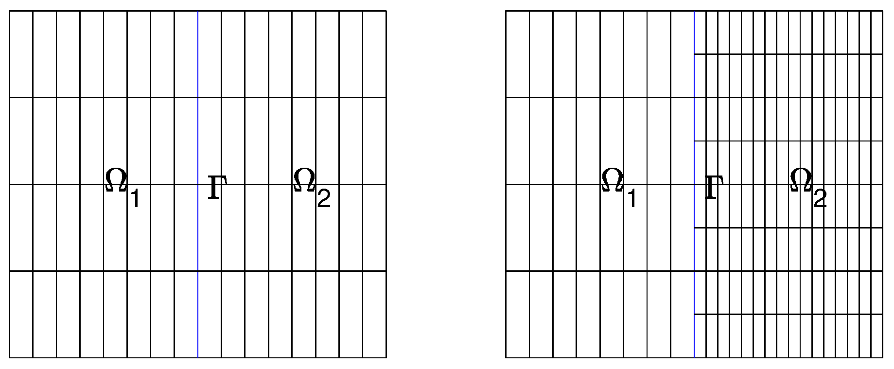
Figure 1.
(Left): quasi-uniform meshes. (Right): piecewise meshes.
Figure 1.
(Left): quasi-uniform meshes. (Right): piecewise meshes.
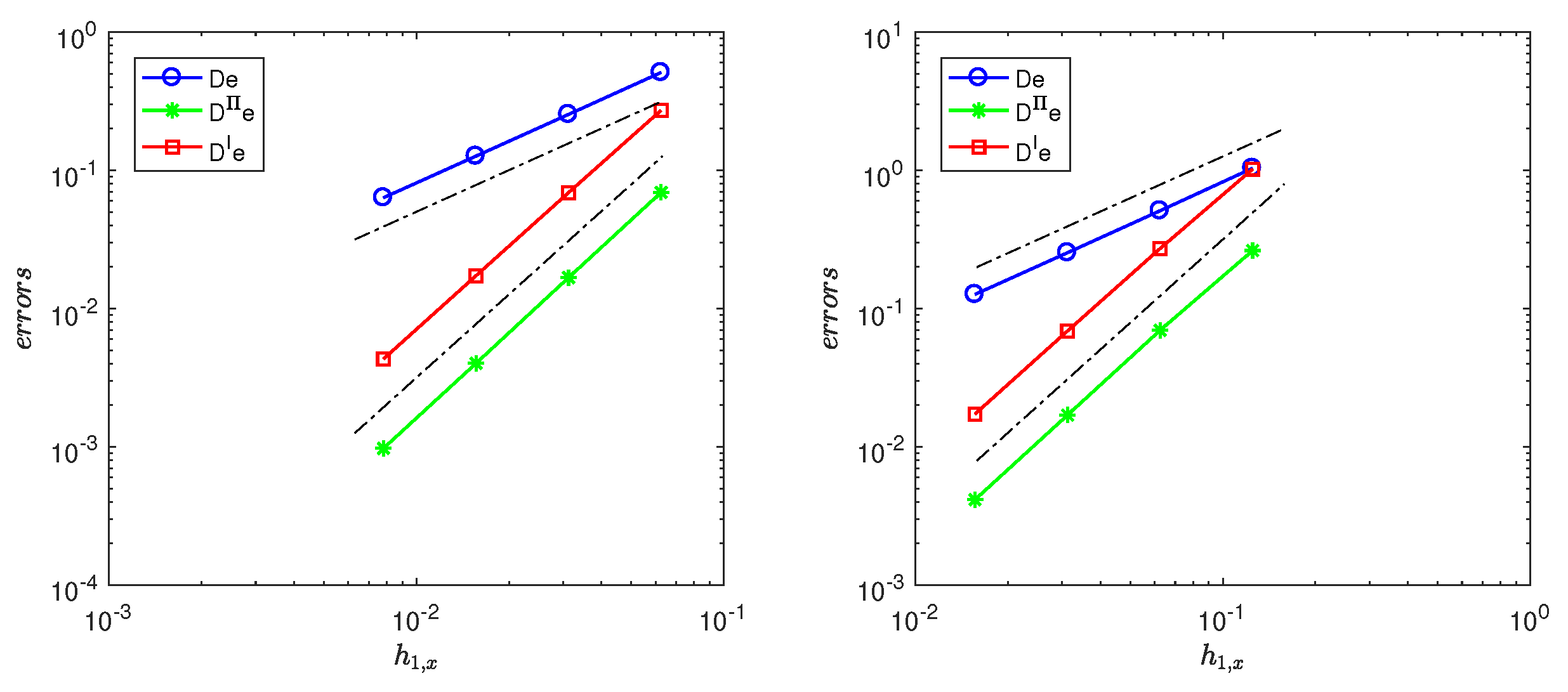
Figure 2.
(Left): Log–log plot of errors , , and versus with based on square quasi-uniform meshes for and for SNIPFEM. The dotted line gives the reference lines of slope 1 and 2. (Right): Log–log plot of errors , , and versus with based on square piecewise meshes and for and for SNIPFEM. The dotted line gives the reference lines of slope 1 and 2.
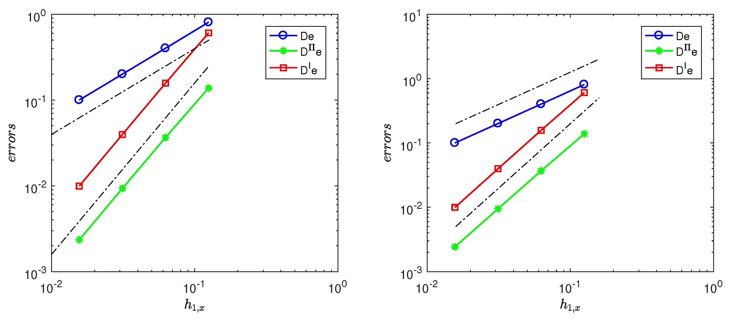
Figure 3.
(Left): Log–log plot of errors , , and versus with based on rectangular quasi-uniform meshes , for and for SNIPFEM. The dotted line gives the reference lines of slope 1 and 2. (Right): Log–log plot of errors , , and versus with based on rectangular piecewise meshes and , for and for SNIPFEM. The dotted line gives the reference lines of slope 1 and 2.
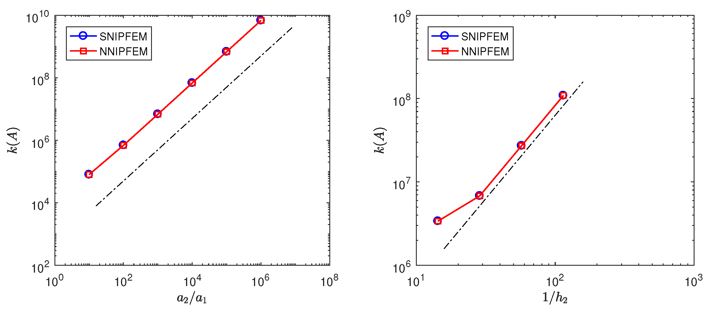
Figure 4.
(Left): Log–log plot of condition number versus with , , , fixed , and for SNIPFEM and NNIPFEM, respectively. The dotted line gives the reference line of slope 1. (Right): Log–log plot of condition number versus with , and fixed , and for SNIPFEM and NNIPFEM, respectively. The dotted line gives the reference line of slope 2.
Table 1.
Rates of errors for Example 1 based on square quasi-uniform and piecewise meshes with and for SNIPFEM.
Table 1.
Rates of errors for Example 1 based on square quasi-uniform and piecewise meshes with and for SNIPFEM.
| | | | | | | |
|---|
| (,) | (,) | 4.6196 | | 7.8364 | | 3.3026 | |
| (,) | (,) | 2.3164 | 0.9958 | 2.2308 | 1.8126 | 9.0132 | 1.8734 |
| (,) | (,) | 1.1580 | 1.0003 | 5.2043 | 2.0998 | 2.3018 | 1.9692 |
| (,) | (,) | 5.7900 | 0.9999 | 1.1042 | 2.2366 | 5.7681 | 1.9966 |
| (,) | (,) | 4.5010 | | 7.9155 | | 3.2036 | |
| (,) | (,) | 2.2559 | 0.9965 | 2.3180 | 1.7717 | 8.7343 | 1.8749 |
| (,) | (,) | 1.1274 | 1.0007 | 5.8135 | 1.9954 | 2.2310 | 1.9689 |
| (,) | (,) | 5.6363 | 1.0001 | 1.4727 | 1.9808 | 5.5966 | 1.9951 |
Table 2.
Rates of errors for Example 1 based on square quasi-uniform and piecewise meshes with and and for NNIPFEM.
Table 2.
Rates of errors for Example 1 based on square quasi-uniform and piecewise meshes with and and for NNIPFEM.
| | | | | | | |
|---|
| (,) | (,) | 4.6394 | | 9.1992 | | 3.3182 | |
| (,) | (,) | 2.3191 | 1.0003 | 2.5519 | 1.8499 | 9.0549 | 1.8736 |
| (,) | (,) | 1.1582 | 1.0016 | 5.8662 | 2.1210 | 2.3102 | 1.9706 |
| (,) | (,) | 5.7902 | 1.0002 | 1.2288 | 2.2551 | 5.7821 | 1.9984 |
| (,) | (,) | 4.5246 | | 9.4562 | | 3.2196 | |
| (,) | (,) | 2.2597 | 1.0016 | 2.7429 | 1.7855 | 8.7770 | 1.8751 |
| (,) | (,) | 1.1280 | 1.0024 | 7.0802 | 1.9538 | 2.2396 | 1.9704 |
| (,) | (,) | 5.6374 | 1.0006 | 1.9158 | 1.8858 | 5.6108 | 1.9969 |
Table 3.
Rates of errors for Example 1 based on rectangular quasi-uniform and piecewise meshes with and for SNIPFEM.
Table 3.
Rates of errors for Example 1 based on rectangular quasi-uniform and piecewise meshes with and for SNIPFEM.
| | | | | | | |
|---|
| (,) | (,) | 3.6234 | | 2.3571 | | 1.9231 | |
| (,) | (,) | 1.8263 | 0.9884 | 6.3468 | 1.8929 | 5.0804 | 1.9204 |
| (,) | (,) | 9.1496 | 0.9971 | 1.5595 | 2.0249 | 1.2884 | 1.9792 |
| (,) | (,) | 4.5770 | 0.9992 | 3.6774 | 2.0843 | 3.2320 | 1.9951 |
| (,) | (,) | 3.5277 | | 2.4795 | | 1.8719 | |
| (,) | (,) | 1.7779 | 0.9884 | 7.4105 | 1.7424 | 4.9452 | 1.9204 |
| (,) | (,) | 8.9066 | 0.9972 | 2.1790 | 1.7658 | 1.2544 | 1.9789 |
| (,) | (,) | 4.4552 | 0.9993 | 6.7520 | 1.6902 | 3.1480 | 1.9945 |
Table 4.
Rates of errors for Example 1 based on rectangular quasi-uniform and piecewise meshes with and for NNIPFEM.
Table 4.
Rates of errors for Example 1 based on rectangular quasi-uniform and piecewise meshes with and for NNIPFEM.
| | | | | | | |
|---|
| (,) | (,) | 3.6307 | | 3.5022 | | 1.9292 | |
| (,) | (,) | 1.8271 | 0.9906 | 8.8727 | 1.9808 | 5.0970 | 1.9203 |
| (,) | (,) | 9.1503 | 0.9976 | 2.0360 | 2.1236 | 1.2917 | 1.9803 |
| (,) | (,) | 4.5771 | 0.9993 | 4.4831 | 2.1831 | 3.2374 | 1.9964 |
| (,) | (,) | 3.5367 | | 3.7686 | | 1.8781 | |
| (,) | (,) | 1.7793 | 0.9910 | 1.0722 | 1.8134 | 4.9621 | 1.9202 |
| (,) | (,) | 8.9087 | 0.9980 | 3.0838 | 1.7978 | 1.2578 | 1.9800 |
| (,) | (,) | 4.4556 | 0.9995 | 9.6200 | 1.6805 | 3.1535 | 1.9958 |
Table 5.
Study of the dependence of the errors for Example 1 on the jump of coefficients with ,,, , and for SNIPFEM and NNIPFEM, respectively.
Table 5.
Study of the dependence of the errors for Example 1 on the jump of coefficients with ,,, , and for SNIPFEM and NNIPFEM, respectively.
| | | | | | |
|---|
| 1.5041 | 9.6301 | 8.9066 | 8.8309 | 8.8233 | 8.8226 |
| 1.2868 | 5.1235 | 2.1790 | 1.5790 | 1.5056 | 1.4981 |
| 1.4935 | 1.2793 | 1.2544 | 1.2519 | 1.2516 | 1.2516 |
| 1.5081 | 9.6426 | 8.9087 | 8.8319 | 8.8241 | 8.8234 |
| 1.7818 | 7.5053 | 3.0838 | 2.1238 | 2.0018 | 1.9892 |
| 1.4922 | 1.2824 | 1.2578 | 1.2552 | 1.2550 | 1.2550 |
Table 6.
Rates of errors for Example 2 based on square quasi-uniform and piecewise meshes with and for NNIPFEM.
Table 6.
Rates of errors for Example 2 based on square quasi-uniform and piecewise meshes with and for NNIPFEM.
| | | | | | | |
|---|
| (,) | (,) | 5.1043 | | 7.3770 | | 2.7228 | |
| (,) | (,) | 2.5368 | 1.0086 | 1.7462 | 2.0787 | 6.9024 | 1.9799 |
| (,) | (,) | 1.2667 | 1.0019 | 4.1175 | 2.0844 | 1.7292 | 1.9969 |
| (,) | (,) | 6.3316 | 1.0004 | 9.8873 | 2.0581 | 4.3221 | 2.0002 |
| (,) | (,) | 1.0409 | | 2.8618 | | 1.0224 | |
| (,) | (,) | 5.1034 | 1.0284 | 7.4612 | 1.9394 | 2.7217 | 1.9094 |
| (,) | (,) | 2.5362 | 1.0087 | 1.7989 | 2.0522 | 6.9001 | 1.9798 |
| (,) | (,) | 1.2663 | 1.0020 | 4.4065 | 2.0294 | 1.7289 | 1.9967 |
Table 7.
Rates of errors for Example 2 based on rectangular quasi-uniform and piecewise meshes with and for NNIPFEM.
Table 7.
Rates of errors for Example 2 based on rectangular quasi-uniform and piecewise meshes with and for NNIPFEM.
| | | | | | | |
|---|
| (,) | (,) | 8.0920 | | 1.4805 | | 6.0783 | |
| (,) | (,) | 4.0160 | 1.0107 | 3.8413 | 1.9464 | 1.5756 | 1.9476 |
| (,) | (,) | 2.0035 | 1.0031 | 9.5984 | 2.0007 | 3.9752 | 1.9868 |
| (,) | (,) | 1.0012 | 1.0008 | 2.3824 | 2.0103 | 9.9597 | 1.9968 |
| (,) | (,) | 8.0907 | | 1.4914 | | 6.0755 | |
| (,) | (,) | 4.0150 | 1.0108 | 3.9040 | 1.9336 | 1.5749 | 1.9476 |
| (,) | (,) | 2.0029 | 1.0032 | 9.9301 | 1.9750 | 3.9735 | 1.9868 |
| (,) | (,) | 1.0008 | 1.0008 | 2.5501 | 1.9612 | 9.9560 | 1.9967 |
Table 8.
Study of the dependence of the errors on the jump of coefficients with , , , , and for SNIPFEM and NNIPFEM, respectively.
Table 8.
Study of the dependence of the errors on the jump of coefficients with , , , , and for SNIPFEM and NNIPFEM, respectively.
| | | | | | |
|---|
| 4.0771 | 4.0199 | 4.0134 | 4.0128 | 4.0127 | 4.0127 |
| 5.3341 | 3.9508 | 3.6929 | 3.6648 | 3.6620 | 3.6617 |
| 1.5806 | 1.5739 | 1.5732 | 1.5731 | 1.5731 | 1.5731 |
| 4.0913 | 4.0237 | 4.0150 | 4.0141 | 4.0140 | 4.0140 |
| 6.5611 | 4.4112 | 3.9040 | 3.8459 | 3.8400 | 3.8394 |
| 1.5814 | 1.5756 | 1.5749 | 1.5749 | 1.5748 | 1.5748 |


