A Totally Relaxed, Self-Adaptive Tseng Extragradient Method for Monotone Variational Inequalities

Abstract

In this work, we study a class of variational inequality problems defined over the intersection of sub-level sets of a countable family of convex functions. We propose a new iterative method for approximating the solution within the framework of Hilbert spaces. The method incorporates several strategies, including inertial effects, a self-adaptive step size, and a relaxation technique, to enhance convergence properties. Notably, it requires computing only a single projection onto a half space. Using some mild conditions, we prove that the sequence generated by our proposed method is strongly convergent to a minimum-norm solution to the problem. Finally, we present some numerical results that validate the applicability of our proposed method.

1. Introduction

Ever since the independent introduction of the classical variational inequality problem (VIP) by Fichera [1] and Stampacchia [2], this field has received great attention from numerous researchers. Let $\mathcal{C}$ be a nonempty, closed and convex subset of a real Hilbert space $\mathcal{H}$ and let $\langle ·,·\rangle$ and $\parallel ·\parallel$ be the inner product and induced norm on $\mathcal{H}$, respectively. The VIP with an operator $\mathcal{F}$ is primarily to find a point $a\in \mathcal{C}$ such that

$$\langle \mathcal{F}\left(a\right),b-a\rangle \ge 0,\forall a\in \mathcal{C}.$$

(1)

We denote the solution set of the VIP (1) by $VI(\mathcal{C},\mathcal{F}).$ The great attention being received by the VIP is due to its applications in so many areas of studies such as optimization, economics, structural analysis, engineering, physics, and operation research (see [3,4,5,6,7,8] and the references therein).

From the fixed point formulation, find $a\in \mathcal{C}$ such that $a=P_{\mathcal{C}}(a-\lambda \mathcal{F}\left(a\right)),$ many projection algorithms for approximating the solution of VIPs have been proposed (for more on fixed point articles, see [9,10,11]). Some of these can be found in [7,12,13,14,15]. The simplest known projection method is the gradient projection method (GPM), which is formulated as

$$a_{m+1}=P_{\mathcal{C}}(a_m-\lambda \mathcal{F}\left(a_m\right)),\forall m>0$$

(2)

where $\lambda$ is a positive real number. This is obtained from the fixed point formulation $a=P_{\mathcal{C}}(a-\lambda \mathcal{F}\left(a\right)).$

This projection method is characterized by some stringent assumptions for its convergence. In a bid to weaken some of these assumptions, Korpelevich [7] proposed the following extragradient method (EgM):

EGM

$$\left\{\begin{array}{c}{a}_0\in \mathcal{C},\hfill \\ b_m=P_{\mathcal{C}}(a_m-\lambda \mathcal{F}\left(a_m\right)),\hfill \\ a_{m+1}=P_{\mathcal{C}}(a_m-\lambda F\left(b_m\right)),\forall m\ge 0\hfill \end{array}\right.$$

(3)

where $\lambda \in (0,{\displaystyle \frac{1}{\mathcal{L}}}),\mathcal{L}$ is the Lipschitz constant of the operator $\mathcal{F}$ and $P_{\mathcal{C}}$ is the metric projection of $\mathcal{H}$ onto $\mathcal{C}$.

Two projections of $\mathcal{H}$ onto the feasible set $\mathcal{C}$ and two evaluations of the cost operator $\mathcal{F}$ that must be performed at each iteration make EgM computationally difficult. This significantly reduces the method’s efficiency and applicability, especially when $\mathcal{F}$ and $\mathcal{C}$ are complex in structure. The authors  [16,17,18,19,20] came up with different modifications to address computational inefficiency of EgM. One of such notable modifications, called the Tseng extragradient method (TEgM), was proposed by Tseng [19]. This method, which is presented as follows, reduced the two projections of the EgM to one:

TEGM

$$\left\{\begin{array}{c}{b}_m=P_{\mathcal{C}}(a_m-\lambda \mathcal{F}\left(a_m\right)),\hfill \\ a_{m+1}=b_m+\lambda (\mathcal{F}\left(a_m\right)-\mathcal{F}\left(b_m\right))\hfill \end{array}\right.$$

(4)

where $\lambda \in (0,{\displaystyle \frac{1}{L}}).$

Another modification was given by Censor et al. [21] with the introduction of the subgradient extragradient method (SEgM), in which the second projection onto $\mathcal{C}$ was replaced with a projection onto a constructible half space, which is one of the subgradient half spaces known to have a simple structure. The following is the method proposed by Censor et al. in [21]:

SEgM

$$\left\{\begin{array}{c}{a}_0\in \mathcal{C},\hfill \\ b_m=P_{\mathcal{C}}(a_m-\lambda \mathcal{F}\left(a_m\right)),\hfill \\ {\mathcal{T}}_m=\{\overline{a}\in \mathcal{H}:\langle a_m-\lambda \mathcal{F}\left(a_m\right)-b_m,\overline{a}-b_m\rangle \le 0\},\hfill \\ a_{m+1}=P_{{\mathcal{T}}_m}(a_m-\lambda \mathcal{F}\left(b_m\right))\hfill \end{array}\right.$$

(5)

where $\lambda \in (0,{\displaystyle \frac{1}{L}}).$

It is clear that the TEgM and SEgM algorithms still have the drawback of calculating a projection onto the feasible set $\mathcal{C}.$ In order to weaken this requirement, Censor et al. [3] proposed the following two-subgradient extragradient method (TSEgM):

TSEgM

$$\left\{\begin{array}{c}{a}_0\in \mathcal{C},\hfill \\ b_m=P_{{\mathcal{T}}_m}(a_m-{\lambda }_m\mathcal{F}\left(a_m\right)),\hfill \\ {\mathcal{T}}_m:=\{\overline{a}\in \mathcal{H}:c\left(a_m\right)+\langle {ϵ}_m,\overline{a}-a_m\rangle \le 0\},\hfill \\ a_{m+1}=P_{{\mathcal{T}}_m}(a_m-\lambda \mathcal{F}\left(b_m\right)),\hfill \end{array}\right.$$

(6)

where ${ϵ}_m\in \partial c\left(a_m\right)$ and $\partial c\left(a\right)$ is the sub-differential of the convex function $c(.)$ at point a defined in (12).

In the TSEgM, the main idea is that any closed and convex set $\mathcal{C}$ can be expressed as

$$\begin{array}{c}\hfill \mathcal{C}=\{a\in \mathcal{H}:c(a)\le 0\},\end{array}$$

(7)

where $c:\mathcal{H}\to \mathbb{R}$ is a convex function. For instance, we can take $c\left(a\right):=\mathrm{dist}(a,\mathcal{C}),$ where “dist” is the distance function. In this method, we observe that two projections are made onto a half space, an advantage that enhances the computational efficiency of the algorithm.

Another method for solving the VIP is the projection and contraction method (PCM), which has been developed by many researchers in the literature (see [22,23,24,25] and the references therein). These PCM algorithms have been shown through numerical experiments to always outperform the EgMs (see [1]). He et al. [14] recently proposed another variant of the projection and contraction algorithm for solving the VIP. The algorithm is as follows:

PCM

$$\left\{\begin{array}{c}{b}_m=P_{{\mathcal{C}}_m}(a_m-{\lambda }_m\mathcal{F}\left(a_m\right))\hfill \\ d(a_m,b_m)=(a_m-b_m)-{\alpha }_m(\mathcal{F}\left(a_m\right)-\mathcal{F}\left(b_m\right))\hfill \\ a_{m+1}^1=a_m-\gamma {\beta }_{m}d(a_m,b_m)\hfill \\ or\hfill \\ a_{m+1}^2=P_{{\mathcal{Q}}_m}(a_m-\gamma {\beta }_m{\lambda }_m\mathcal{F}\left(b_m\right))\hfill \\ {\mathcal{C}}_m:=\{\overline{a}\in \mathcal{H}:c\left(a_m\right)+\langle c^{\prime }\left(a_m\right),\overline{a}-a_m\rangle \le 0\}\hfill \\ {\mathcal{Q}}_m:=\{\overline{a}\in \mathcal{H}:\langle \overline{a}-b_m,{\lambda }_m\mathcal{F}{b}_m-d(a_m-b_m)\rangle \ge 0\}\hfill \end{array}\right.$$

(8)

where ${\mathcal{C}}_m$ and ${\mathcal{Q}}_m$ are half spaces, $\gamma \in (0,2)$ is a relaxation factor, ${\lambda }_m$ is the production step size and ${\beta }_m$ is the optimal correction step length.

Iterative methods with an improved rate of convergence for solving the problems of optimization have received great attention from many researchers recently. The inertial and relaxation techniques are the two commonly used techniques researchers employ to speed up the rate of convergence of algorithms. The inertial technique, which was introduced by Polyak [26], has been used by many authors, few of whom are in [12,13,16,27]. The relaxation method, on the other hand, has also been adopted by many researchers; see [28,29,30]. The authors in [30] investigated the effect of these two techniques on the convergence properties of iterative schemes.

Cao and Guo [27] modified the work of Censor et al. in [3], with the addition of an inertial technique, and so proposed the following inertial two-subgradient extragradient algorithm for solving the VIP:

ITSEgM

$$\left\{\begin{array}{c}{s}_m=a_m+{\theta }_m(a_m-a_{m-1}),\hfill \\ {\mathcal{C}}_m:=\{\overline{a}\in \mathcal{H}:c\left(a_m\right)+\langle {ϵ}_m,\overline{a}-a_m\rangle \le 0\},\hfill \\ b_m=P_{{\mathcal{C}}_m}(s_m-\lambda \mathcal{F}\left(s_m\right)),\hfill \\ a_{m+1}:=P_{{\mathcal{C}}_m}(a_m-\lambda \mathcal{F}\left(b_m\right))\ge 0\}\hfill \end{array}\right.$$

(9)

where $\lambda >0$ and ${\theta }_m\ge 0.$

In this research, our interest is in studying the VIPs where the feasible set $\mathcal{C}$ is given as a finite intersection of sub-level sets of convex functions defined as follows:

$$\mathcal{C}:=\bigcap _{i=1}^k{\mathcal{C}}^i:=\{z\in \mathcal{H}:c_i\left(z\right)\le 0\},$$

(10)

where k is a positive integer and $c_i:\mathcal{H}\to \mathbb{R}$ for all $i\in I:=\{1,2,\dots ,k\}$ are convex functions.

In recent times, He et al. [31] proposed a new iterative algorithm called the totally relaxed and self-adaptive subgradient extragradient method (TRSSEM) for solving VIP. The algorithm is as follows:

TRSSEM

$$\left\{\begin{array}{c}{a}_0\in \mathcal{H},\hfill \\ {\mathcal{C}}_m^i:=\{a\in \mathcal{H}:c_i\left(a_m\right)+\langle c_i^{\prime }\left(a_m\right),a-a_m\}\le 0\},\hfill \\ {\mathcal{C}}_m:=\bigcap {\mathcal{C}}_m^i,\hfill \\ b_m=P_{{\mathcal{C}}_m}(a_m-{\beta }_m\mathcal{F}\left(a_m\right)),\hfill \\ {\beta }_m^2\parallel \mathcal{F}\left(a_m\right)-\mathcal{F}\left(b_m\right){\parallel }^2+M^{\prime }{\beta }_m\parallel a_m-b_m{\parallel }^2\le v^2\parallel a_m-b_m\parallel ,\hfill \\ a_{m+1}=P_{{\mathcal{C}}_m}(a_m-{\beta }_m\mathcal{F}\left(b_m\right))\mathrm{or},\hfill \\ a_{m+1}=P_{{\mathcal{T}}_m}(a_m-{\beta }_m\mathcal{F}\left(b_m\right)\hfill \end{array}\right.$$

(11)

where ${\beta }_m=\sigma {\rho }^{lm},\sigma >0,\rho \in (0,1),M^{\prime }=ML,$$L=max\left\{Li\right|i\in I\}$ and

$$\begin{array}{cc}\hfill {\mathcal{T}}_m:=& \left\{\begin{array}{c}\{a\in \mathcal{H}:\langle a_m,a-b_m\rangle \le 0\}\mathrm{if}{a}_m\ne 0,\hfill \\ \mathcal{H}\mathrm{if}{a}_m=0\hfill \end{array}\right.\hfill \end{array}$$

$v\in (0,1).$

A weak convergent result of the proposed method in the framework of Hilbert spaces was obtained by the authors in [31].

This paper is motivated by the above studies, which necessitated our proposed study on inertial and relaxation methods for solving the VIP in the framework of Hilbert spaces. The following are the important features of our algorithm:

• The combination of the inertial and relaxation techniques for speeding up the convergence rate the iterative scheme.
• The presence of a simple self-adaptive stepsize, which is generated at each iteration by some simple computations.
• The algorithm is independent of the use of the Lipschitz continuity assumption which is commonly employed by authors when solving the monotone variational inequality problem (MVIP).
• Strong convergence of the generated sequence to a minimum-norm solution to the problems.
• Computation of only one projection onto some half space.

The organization of the paper is as follows: Section 2 contains some recalled definitions and well-known lemmas needed for our analysis. Section 3 consists of our proposed algorithm, Section 4 accommodates strong convergence analysis of the algorithm, while in Section 5, there are numerical experiments used to validate our results, and the concluding remarks are given in Section 6.

2. Preliminaries

Let $\mathcal{C}$ be a nonempty, closed and convex subset of a real Hilbert space $\mathcal{H}.$ The weak convergence and strong convergence of $\left\{a_m\right\}$ to a are represented by $a_m\rightharpoonup a$ and $a_m\to a,$ respectively, and $w_{\omega }\left(a_m\right)$ denotes the set of weak limits of $\left\{a_m\right\},$ that is,

$$w_{\omega }\left(a_m\right)=\{a\in H:a_{m_j}\rightharpoonup a\mathrm{for}\mathrm{some}\mathrm{subsequence}\left\{a_{m_j}\right\}\mathrm{of}\left\{a_m\right\}\}.$$

Definition 1.

Let $\mathcal{H}$ be a real Hilbert space $\mathcal{H}$. The mapping $\mathcal{F}:\mathcal{H}\to \mathcal{H}$ is said to be

(1) $\mathcal{L}$-Lipschitz-continuous, where $\mathcal{L}>0,$ if

$$\parallel \mathcal{F}a-\mathcal{F}b\parallel \le \mathcal{L}\parallel a-b\parallel ,\forall a,b\in \mathcal{H}.$$

If $\mathcal{L}\in [0,1),$ then $\mathcal{F}$ is a contraction;

(2) nonexpansive, if $\mathcal{F}$ is 1-Lipschitz continuous.

Definition 2.

Given a mapping $\mathcal{F}:\mathcal{H}\to \mathcal{H}$, F is called monotone if 

$$\langle \mathcal{F}a-\mathcal{F}b,a-b\rangle \ge 0,\forall a,b\in \mathcal{H}.$$

Definition 3.

([32]). A function $c:\mathcal{H}\to \mathbb{R}$ is said to be G$\widehat{a}$teaux-differentiable at $a\in \mathcal{H}$ if there exists an element denoted by $c^{\prime }\left(a\right)\in \mathcal{H}$ such that

$$\begin{array}{c}\hfill \underset{h\to 0}{lim}{\displaystyle \frac{c(a+bh)-c\left(a\right)}{h}}=\langle b,c^{\prime }\left(a\right)\rangle ,\forall b\in \mathcal{H},h\in [0,1],\end{array}$$

where $c^{\prime }\left(a\right)$ is called the G$\widehat{a}$teaux differential of c at a. Recall that if for each $a\in \mathcal{H}$, c is G$\widehat{a}$teaux differentiable at a, then c is G$\widehat{a}$teaux-differentiable on $\mathcal{H}$.

Definition 4.

([32]). Let c be a convex function. $c:\mathcal{H}\to \mathbb{R}$ is said to be subdifferentiable at a point $a\in \mathcal{H}$ if the set

$$\begin{array}{c}\hfill \partial c\left(a\right)=\{\zeta \in \mathcal{H}:c(b)\ge c(a)+\langle \zeta ,b-a\rangle ,\forall b\in \mathcal{H}\}\end{array}$$

(12)

is nonempty. Each element in $\partial c\left(a\right)$ is called a subgradient of c at a. We note that if c is subdifferentiable at each $a\in \mathcal{H}$, then c is subdifferentiable on $\mathcal{H}$. It is also known that if c is G$\widehat{a}$teaux-differentiable at a, then c is subdifferentiable at a and $\partial c\left(a\right)=\left\{c^{\prime }\left(a\right)\right\}$.

Definition 5.

Let $\mathcal{H}$ be a real Hilbert space. A function $c:\mathcal{H}\to \mathbb{R}\cup \{+\infty \}$ is said to be weakly lower semi-continuous (w-lsc) at $a\in \mathcal{H},$ if

$$c\left(a\right)\le \underset{m\to \infty }{lim\; inf}c\left(a_m\right)$$

holds for every sequence $\left\{a_m\right\}$ in $\mathcal{H}$ satisfying $a_m\rightharpoonup a.$

Lemma 1.

Let $\mathcal{H}$ be a real Hilbert space such that $a,b\in \mathcal{H}.$ Then, the following results hold:

(i) 

$2\langle a,b\rangle ={\parallel a\parallel }^2+{\parallel b\parallel }^2{-\parallel a-b\parallel }^2={\parallel a+b\parallel }^2-{\parallel a\parallel }^2-{\parallel b\parallel }^2;$

(ii) 

${\parallel a+b\parallel }^2\le {\parallel a\parallel }^2+2\langle b,a+b\rangle ;$

(iii) 

  If $\alpha ,\beta \in [0,1]$ with $\alpha +\beta =1,$ we have

$${\parallel \alpha a+\beta b\parallel }^2={\alpha \parallel a\parallel }^2+{\beta \parallel b\parallel }^2-\alpha \beta {\parallel a-b\parallel }^2.$$

Lemma 2.

Let $\mathcal{C}$ be a nonempty, closed, and convex subset of H. Suppose $\mathcal{F}:\mathcal{C}\to \mathcal{H}$ is a continuous monotone mapping and $\overline{a}\in \mathcal{C}$; then,

$$\overline{a}\in VI(\mathcal{C},\mathcal{F})\iff \langle \mathcal{C}\left(a\right),a-\overline{a}\rangle \ge 0\forall a\in \mathcal{C}.$$

Lemma 3.

([33]). Let $\mathcal{C}$ be a set defined as in (10), and let $\mathcal{F}:h\to \mathcal{H}$ be an operator. Suppose the solution set $VI(\mathcal{C},\mathcal{F})$ is nonempty. Then, the following alternating theorem holds for the solution of the $VI(\mathcal{C},\mathcal{F})$, that is, given $\hat{a}\in \mathcal{C},\hat{a}\in VI(\mathcal{C},\mathcal{F})$, if and only if one of the following holds.

(i) 

$\mathcal{F}\widehat{a}=0,$ or

(ii) 

$\widehat{a}\in bd\left(\mathcal{C}\right),$ and there exist ${\beta }_{\widehat{a}}>0$ (depending on the point $\widehat{a}$) and $\kappa \in conv\{c_i^{\prime }\left(\widehat{a}\right):i\in I_{\widehat{a}}^{*}\}$ such that $\mathcal{F}\left(\widehat{a}\right)=-{\beta }_{\widehat{a}}\kappa ,$ where $bd\left(\mathcal{C}\right)$ denotes the boundary of the set $\mathcal{C},$$I_{\kappa }^{*}=\{i\in I:c_i\left(\widehat{a}\right)=0\}$ and $conv\{c_i^{\prime }\left(\widehat{a}\right):i\in I_{\widehat{a}}^{*}\}$ is the convex hull of the set $\{c_i^{\prime }\left(\widehat{a}\right):i\in I_{\widehat{a}}^{*}\}.$

Lemma 4.

([34]). Let $\left\{a_m\right\}$ be a sequence of non-negative real numbers, $\left\{{\alpha }_m\right\}$ be a sequence in $(0,1)$ with ${\sum }_{m=1}^{\infty }{\alpha }_m=\infty$ and $\left\{b_m\right\}$ be a sequence of real numbers. Assume that

$$a_{m+1}\le (1-{\alpha }_m)a_m+{\alpha }_m{b}_m,\mathrm{for}\mathrm{all}m\ge 1,$$

and if ${lim\; sup}_{k\to \infty }{b}_{m_k}\le 0$ for every subsequence $\left\{a_{m_k}\right\}$ of $\left\{a_m\right\}$ satisfying ${lim\; inf}_{k\to \infty }(a_{m_{k+1}}-a_{m_k})\ge 0,$ then ${lim}_{m\to \infty }{a}_m=0.$

Lemma 5.

([35]). Suppose $\left\{{\lambda }_m\right\}$ and $\left\{{\mu }_m\right\}$ are two nonnegative real sequences such that

$${\lambda }_{m+1}\le {\lambda }_m+{\mu }_m,\forall m\ge 1.$$

If ${\sum }_{m=1}^{\infty }{\mu }_m<+\infty ,$ then $\underset{m\to \infty }{lim}{\lambda }_m$ exists.

3. Proposed Algorithm

We present our proposed algorithm in this section and give the conditions for its convergence.

Assumption 1.

(1) 

The solution set $VI(\mathcal{C},\mathcal{F})$ is nonempty.

(2) 

The mapping $\mathcal{F}:\mathcal{H}⟶\mathcal{H}$ is monotone and $\mathcal{L}$-Lipschitz-continuous on $\mathcal{H}$.

(3) 

For all $i\in I$, the family of functions $c_i:\mathcal{H}\to \mathbb{R}$ satisfy the following conditions.

(i) 

Any $c_i(i\in I)$ is convex on $\mathcal{H}$.

(ii) 

Any $c_i(i\in I)$ is weakly lower semi-continuous on $\mathcal{H}.$

(iii) 

Any $c_i(i\in I)$ is Gâteaux-differentiable and $c_i^{\prime }(i\in I)$ is ${\mathcal{L}}_i$-Lipschitz-continuous on $\mathcal{H}.$

(iv) 

There exists a positive constant M such that for all $\widehat{a}\in bd\left(\mathcal{C}\right),$ the following holds:

$$\parallel \mathcal{F}\widehat{a}\parallel \le Minf\{\parallel m\left(\widehat{a}\right)\parallel :m\left(\widehat{a}\right)\in \mathrm{con}\{c_i^{\prime }\left(\widehat{a}\right):i\in I_{\widehat{a}}^{*}\}\},$$

where $I_{\widehat{a}}^{*}$ is defined as in Lemma 3.

(4) 

${\left\{{\alpha }_m\right\}}_{m=1}^{\infty },{\left\{{\beta }_m\right\}}_{m=1}^{\infty }$ and ${\left\{{\xi }_m\right\}}_{m=1}^{\infty }$ are non-negative sequences satisfying the following conditions:

(i) 

${\alpha }_m\in (0,1),$$\underset{m\to \infty }{lim}{\alpha }_m=0,{\sum }_{m=1}^{\infty }{\alpha }_m=+\infty ,\underset{m\to \infty }{lim}{\displaystyle \frac{{\xi }_m}{{\alpha }_m}}=0.$

(ii) 

$\left\{{\beta }_m\right\}\subset [a,b]\subset (0,1-{\alpha }_m),\left\{{\varphi }_m\right\}\subset (0,1]$ such that $\underset{m\to +\infty }{lim}{\varphi }_m=\varphi \in (0,1].$

(iii) 

$0<\delta <{\displaystyle \frac{2\varphi -M-2+\sqrt{M^2+4M(1-\varphi )+4}}{2\varphi }}.$

(iv) 

Let $\left\{{\sigma }_m\right\}$ be a nonnegative sequence such that ${\sum }_{m=1}^{\infty }{\sigma }_m<+\infty .$

The following is the proposed algorithm (Algorithm 1):

Algorithm 1: TRSTEM

Initialization: Given $\theta >0,{\lambda }_1>0.$ Let $a_0,a_1\in \mathcal{H}$ be two initial points and set $m=1.$ Given the $(m-1)th$ and $mth$ iterates, choose ${\theta }_m$ such that $0\le {\theta }_m\le {\widehat{\theta }}_m$ with ${\widehat{\theta }}_m$ defined by $${\widehat{\theta }}_m=\left\{\begin{array}{c}\min \left\{\theta ,{\displaystyle \frac{{\xi }_m}{\parallel a_m-a_{m-1}\parallel }}\right\},\mathrm{if}{a}_m\ne a_{m-1},\hfill \\ \theta ,\mathrm{otherwise}.\hfill \end{array}\right.$$ (13) Iterative steps: Calculate the next iterate $a_{m+1}$ as follows: $$\left\{\begin{array}{c}{s}_m=a_m+{\theta }_m(a_m-a_{m-1}),\hfill \\ {\mathcal{C}}_m^i=\left\{a\in H:c_i\left(s_m\right)+\langle c_i^{\prime }\left(s_m\right),a-s_m\rangle \le 0\right\},i\in I,\hfill \\ {\mathcal{C}}_m:=\bigcap _{i\in I}{\mathcal{C}}_m^i,\hfill \\ b_m=P_{{\mathcal{C}}_m}(s_m-{\lambda }_m\mathcal{F}{s}_m),\hfill \\ e_m=(1-{\varphi }_m)s_m+{\varphi }_m(b_m+{\lambda }_m(\mathcal{F}{s}_m-\mathcal{F}{b}_m)),\hfill \\ a_{m+1}=(1-{\alpha }_m-{\beta }_m)s_m+{\beta }_m{e}_m\hfill \end{array}\right.$$ (14) where $$\hspace{1em} {\lambda }_{m+1}=\left\{\begin{array}{cc}\min \left\{{\displaystyle \frac{\delta \parallel s_m-b_m\parallel }{\parallel \mathcal{F}{s}_m-\mathcal{F}{b}_m\parallel +\parallel c_i^{\prime }\left(s_m\right)-c_i^{\prime }\left(b_m\right)\parallel }},{\lambda }_m+{\sigma }_m\right\},\hfill & \mathrm{if}\parallel \mathcal{F}{s}_m-\mathcal{F}{b}_m\parallel +\parallel c_i^{\prime }\left(s_m\right)-c_i^{\prime }\left(b_m\right)\parallel \ne 0,\hfill \\ {\lambda }_m+{\sigma }_m,\hfill & \mathrm{otherwise},\hfill \end{array}\right.$$ (15) where $\parallel c_i^{\prime }\left(s_m\right)-c_i^{\prime }\left(b_m\right)\parallel =\underset{i\in I}{max}\left\{\parallel c_i^{\prime }\left(s_m\right)-c_i^{\prime }\left(b_m\right)\parallel \right\}.$

Remark 1.

• We do not require the knowledge of the Lipschitz constant of the cost operator $\mathcal{F}$ or the Lipschitz constant of each G$\widehat{a}$teaux differential $c_i^{\prime }(·)$ of $c_i(·)$ to implement our proposed algorithm, as most often used by some researchers (for instance, see [27]).
• Computation of only one projection onto some half space is another feature of our algorithm that makes it computationally efficient to implement.

Remark 2.

Observe that, by Assumption 1 4(i), it can easily be verified from (13) that

$$\underset{m\to \infty }{lim}{\theta }_m\parallel a_m-a_{m-1}\parallel =0\mathrm{and}\underset{m\to \infty }{lim}{\displaystyle \frac{{\theta }_m}{{\alpha }_m}}\parallel a_m-a_{m-1}\parallel =0.$$

4. Convergence Analysis

Here, we start with some relevant lemmas needed to establish the strong convergence theorem of our proposed algorithm.

Lemma 6.

Suppose $\mathcal{C}$ and ${\mathcal{C}}_m$ are the sets defined by (10) and (14), respectively. Then, we have that $\mathcal{C}\subset {\mathcal{C}}_m,\forall m\ge 1.$

Proof. 

For all $i\in I$, let ${\mathcal{C}}^i:=\{a\in \mathcal{H}:c_i\left(a\right)\le 0\}$. Thus, we see that $\mathcal{C}={\bigcap }_{i\in I}{\mathcal{C}}^i$. Then, for each $i\in I$ and any $a\in {\mathcal{C}}^i,$ by the subdifferential inequality, it follows that

$$c_i\left(s_m\right)+\langle c_i^{\prime }\left(s_m\right),a-s_m\rangle \le c_i\left(a\right)\le 0.$$

(16)

By definition of the sets ${\mathcal{C}}_m^i$ (14), we see that $a\in {\mathcal{C}}_m^i.$ It then follows that ${\mathcal{C}}^i\subset {\mathcal{C}}_m^i,\forall m\ge 1,i\in I.$ Therefore, $\mathcal{C}\subset {\mathcal{C}}_m,\forall m\ge 1$ as required. □

Lemma 7.

Let $\left\{{\lambda }_m\right\}$ be a sequence generated by Algorithm 1. Then, $\left\{{\lambda }_m\right\}$ is well defined and $\underset{m\to \infty }{lim}{\lambda }_m=\lambda ,$ where $\lambda \in \left[min\{{\displaystyle \frac{\delta }{K}},{\lambda }_1\},{\lambda }_1+\sigma \right],$ for some positive constant K and $\sigma ={\sum }_{m=1}^{\infty }{\sigma }_m.$

Proof. 

By the Lipschitz continuity of $\mathcal{F}$ and and each $c_i^{\prime }(·),$$\parallel \mathcal{F}{s}_m-\mathcal{F}{b}_m\parallel +\parallel c_i^{\prime }\left(s_m\right)-c_i^{\prime }\left(b_m\right)\parallel \ne 0$, for all $m\ge 1$, we have

$$\begin{array}{cc}\hfill {\displaystyle \frac{\delta \parallel s_m-b_m\parallel }{\parallel \mathcal{F}{w}_{-}\mathcal{F}{b}_m\parallel +\parallel c_i^{\prime }\left(s_m\right)-c_i^{\prime }\left(b_m\right)\parallel }}& \ge {\displaystyle \frac{\delta \parallel s_m-b_m\parallel }{\mathcal{L}\parallel s_m-b_m\parallel +\widehat{\mathcal{L}}\parallel s_m-b_m\parallel }}\hfill \\ \hfill & ={\displaystyle \frac{\delta }{K}},\hfill \end{array}$$

where $\widehat{\mathcal{L}}=max\{{\mathcal{L}}_i:i\in I\},K=\mathcal{L}+\widehat{\mathcal{L}}.$ Clearly, from the definition of ${\lambda }_{m+1},$ the sequence $\left\{{\lambda }_m\right\}$ has lower bound $min\{{\displaystyle \frac{\delta }{K}},{\lambda }_1\}$ and upper bound ${\lambda }_1+\sigma .$ By Lemma 5, we have that $\underset{n\to \infty }{lim}{\lambda }_m$ exists and we denote $\lambda =\underset{m\to \infty }{lim}{\lambda }_m.$ It is clear that $\lambda \in \left[min\{{\displaystyle \frac{\delta }{K}},{\lambda }_1\},{\lambda }_1+\sigma \right].$ □

Lemma 8.

Let $p\in VI(\mathcal{C},\mathcal{F})$ and $\left\{a_m\right\}$ be a sequence generated by Algorithm 1 under Assumption 1. Then, we have the following inequality:

$$\parallel e_m{-p\parallel }^2\le \parallel s_m{-p\parallel }^2-{\varphi }_m\left[2-{\varphi }_m-{\varphi }_m{\delta }^2{\displaystyle \frac{{\lambda }_m^2}{{\lambda }_{m+1}^2}}-2(1-{\lambda }_m)\delta {\displaystyle \frac{{\lambda }_m}{{\lambda }_{m+1}}}-M\delta {\displaystyle \frac{{\lambda }_m}{{\lambda }_{m+1}}}\right]{\parallel s_m-b_m\parallel }^2.$$

(17)

Proof. 

From (15), we have

$$\begin{array}{cc}\hfill {\lambda }_{m+1}& =min\left\{{\displaystyle \frac{\delta \parallel s_m-b_m\parallel }{\parallel \mathcal{F}{s}_m-\mathcal{F}{b}_m\parallel +\parallel c_i^{\prime }\left(s_m\right)-c_i^{\prime }\left(b_m\right)\parallel }},{\lambda }_m+{\sigma }_m\right\}\hfill \\ \hfill & \le {\displaystyle \frac{\delta \parallel s_m-b_m\parallel }{\parallel \mathcal{F}{s}_m-\mathcal{F}{b}_m\parallel +\parallel c_i^{\prime }\left(s_m\right)-c_i^{\prime }\left(b_m\right)\parallel }},\hfill \end{array}$$

(18)

which implies that

$$\begin{array}{c}\hfill \parallel \mathcal{F}{s}_m-\mathcal{F}{b}_m\parallel +\parallel c_i^{\prime }\left(s_m\right)-c_i^{\prime }\left(b_m\right)\parallel \le {\displaystyle \frac{\delta }{{\lambda }_{m+1}}}\parallel s_m-b_m\parallel ,\forall m\ge 1.\end{array}$$

(19)

Assume $p\in VI(\mathcal{C},\mathcal{F}).$ Then, $p\in \mathcal{C}\subset {\mathcal{C}}_m.$ Since $b_m=P_{{\mathcal{C}}_m}(s_m-{\lambda }_m\mathcal{F}{s}_m)$ and $p\in {\mathcal{C}}_m,$ then by the characterization of $P_{{\mathcal{C}}_m}$ we obtain

$$\langle s_m-{\lambda }_m\mathcal{F}{s}_m-b_m,b_m-p\rangle \ge 0,$$

which is equivalent to

$$2\langle s_m-b_m,b_m-p\rangle -2{\lambda }_m\langle \mathcal{F}{s}_m-\mathcal{F}{b}_m,b_m-p\rangle -2{\lambda }_m\langle \mathcal{F}{b}_m,b_m-p\rangle \ge 0.$$

(20)

Using Lemma 1(i), we have

$$2\langle s_m-b_m,b_m-p\rangle = \parallel s_m{-p\parallel }^2-\parallel s_m-b_m{\parallel }^2-{\parallel b_m-p\parallel }^2.$$

(21)

By the monotonicity of $\mathcal{F}$, we obtain

$$\begin{array}{cc}\hfill \langle \mathcal{F}{b}_m,b_m-p\rangle & =\langle \mathcal{F}{b}_m-Fp,b_m-p\rangle +\langle \mathcal{F}p,b_m-p\rangle \hfill \\ \hfill & \ge \langle \mathcal{F}p,b_m-p\rangle .\hfill \end{array}$$

(22)

Substituting (21) and (22) into (20), we have

$$\parallel b_m{-p\parallel }^2\le \parallel s_m{-p\parallel }^2-{\parallel s_m-b_m\parallel }^2-2{\lambda }_m\langle \mathcal{F}{s}_m-\mathcal{F}{b}_m,b_m-p\rangle +2{\lambda }_m\langle \mathcal{F}p,p-b_m\rangle .$$

(23)

Now using the definition of $e_m$ together with Lemma 1, we obtain

$$\begin{array}{cc}\hfill \parallel e_m{-p\parallel }^2& = \parallel (1-{\varphi }_m)s_m+{\varphi }_m{b}_m+{\varphi }_m{\lambda }_m(\mathcal{F}{s}_m-\mathcal{F}{b}_m){-p\parallel }^2\hfill \\ \hfill & = \parallel (1-{\varphi }_m)(s_m-p)+{\varphi }_m(b_m-p)+{\varphi }_m{\lambda }_m(\mathcal{F}{s}_m-\mathcal{F}{b}_m){\parallel }^2\hfill \\ \hfill & ={(1-{\varphi }_m)}^2\parallel s_m{-p\parallel }^2+{\varphi }_m^2\parallel b_m{-p\parallel }^2+{\varphi }_m^2{\lambda }_m^2{\parallel \mathcal{F}{s}_m-\mathcal{F}{b}_m\parallel }^2\hfill \\ \hfill & + 2{\varphi }_m(1-{\varphi }_m)\langle s_m-p,b_m-p\rangle +2{\lambda }_m{\varphi }_m(1-{\varphi }_m)\langle s_m-p,\mathcal{F}{s}_m-\mathcal{F}{b}_m\rangle \hfill \\ \hfill & + 2{\lambda }_m{\varphi }_m^2\langle b_m-p,\mathcal{F}{s}_m-\mathcal{F}{b}_m\rangle \hfill \\ \hfill & ={(1-{\varphi }_m)}^2\parallel s_m{-p\parallel }^2+{\varphi }_m(1-{\varphi }_m)[\parallel s_m{-p\parallel }^2+{\parallel b_m-p\parallel }^2\hfill \\ \hfill & +{\varphi }_m^2\parallel b_m{-p\parallel }^2+{\varphi }_m^2{\lambda }_m^2{\parallel \mathcal{F}{s}_m-\mathcal{F}{b}_m\parallel }^2\hfill \\ \hfill & - \parallel s_m-b_m{\parallel }^2]+2{\lambda }_m{\varphi }_m(1-{\varphi }_m)\langle s_m-p,\mathcal{F}{s}_m-\mathcal{F}{b}_m\rangle +2{\lambda }_m{\varphi }_m^2\langle b_m-p,\mathcal{F}{s}_m-\mathcal{F}{b}_m\rangle \hfill \\ \hfill & =(1-{\varphi }_m)\parallel s_m{-p\parallel }^2+{\varphi }_m\parallel b_m{-p\parallel }^2-{\varphi }_m(1-{\varphi }_m)\parallel s_m-b_m{\parallel }^2+{\varphi }_m^2{\lambda }_m^2{\parallel \mathcal{F}{s}_m-\mathcal{F}{b}_m\parallel }^2\hfill \\ \hfill & + 2{\lambda }_m{\varphi }_m(1-{\varphi }_m)\langle s_m-p,\mathcal{F}{s}_m-\mathcal{F}{b}_m\rangle +2{\lambda }_m{\varphi }_m^2\langle b_m-p,\mathcal{F}{s}_m-\mathcal{F}{b}_m\rangle .\hfill \end{array}$$

(24)

Applying (23) in (24) gives

$$\begin{array}{cc}\hfill \parallel e_m{-p\parallel }^2& \le (1-{\varphi }_m)\parallel s_m{-p\parallel }^2+{\varphi }_m[\parallel s_m{-p\parallel }^2-{\parallel s_m-b_m\parallel }^2-2{\lambda }_m\langle \mathcal{F}{s}_m-\mathcal{F}{b}_m,b_m-p\rangle \hfill \\ \hfill & +2{\lambda }_m\langle Fp,p-b_m\rangle ]-{\varphi }_m(1-{\varphi }_m)\parallel s_m-b_m{\parallel }^2+{\varphi }_m^2{\lambda }_m^2{\parallel \mathcal{F}{s}_m-\mathcal{F}{b}_m\parallel }^2\hfill \\ \hfill & + 2{\varphi }_m(1-{\varphi }_m){\lambda }_m\langle s_m-p,\mathcal{F}{s}_m-\mathcal{F}{b}_m\rangle +2{\varphi }_m^2\langle b_m-p,\mathcal{F}{s}_m-\mathcal{F}{b}_m\rangle \hfill \\ \hfill & = \parallel s_m{-p\parallel }^2-{\varphi }_m(2-{\varphi }_m)\parallel s_m-b_m{\parallel }^2+{\varphi }_m^2{\lambda }_m^2{\parallel \mathcal{F}{s}_m-\mathcal{F}{b}_m\parallel }^2\hfill \\ \hfill & + 2{\lambda }_m{\varphi }_m(1-{\varphi }_m)\langle \mathcal{F}{s}_m-\mathcal{F}{b}_m,s_m-b_m\rangle +2{\lambda }_m{\varphi }_m\langle Fp,p-b_m\rangle .\hfill \end{array}$$

(25)

Now, we consider the following two cases:

Case 1:$\mathcal{F}p=0.$ If $\mathcal{F}p=0,$ then from (25) and by applying (19), we have

$$\begin{array}{cc}\hfill \parallel e_m{-p\parallel }^2& \le \parallel s_m{-p\parallel }^2-{\varphi }_m(2-{\varphi }_m)\parallel s_m-b_m{\parallel }^2+{\varphi }_m^2{\lambda }_m^2{\parallel \mathcal{F}{s}_m-\mathcal{F}{b}_m\parallel }^2\hfill \\ & + 2{\lambda }_m{\varphi }_m(1-{\varphi }_m)\langle \mathcal{F}{s}_m-\mathcal{F}{b}_m,s_m-b_m\rangle \hfill \\ \hfill & \le \parallel s_m{-p\parallel }^2-{\varphi }_m(2-{\varphi }_m)\parallel s_m-b_m{\parallel }^2+{\varphi }_m^2{\delta }^2{\displaystyle \frac{{\lambda }_m^2}{{\lambda }_{m+1}^2}}{\parallel s_m-b_m\parallel }^2\hfill \\ & + 2{\varphi }_m(1-{\varphi }_m)\delta {\displaystyle \frac{{\lambda }_m}{{\lambda }_{m+1}}}{\parallel s_m-b_m\parallel }^2\hfill \\ \hfill & = \parallel s_m{-p\parallel }^2-{\varphi }_m\left[2-{\varphi }_m-{\varphi }_m{\delta }^2{\displaystyle \frac{{\lambda }_m^2}{{\lambda }_{m+1}^2}}-2(1-{\lambda }_m)\delta {\displaystyle \frac{{\lambda }_m}{{\lambda }_{m+1}}}\right]{\parallel s_m-b_m\parallel }^2\hfill \\ \hfill & \le \parallel s_m{-p\parallel }^2-{\varphi }_m\left[2-{\varphi }_m-{\varphi }_m{\delta }^2{\displaystyle \frac{{\lambda }_m^2}{{\lambda }_{m+1}^2}}-2(1-{\lambda }_m)\delta {\displaystyle \frac{{\lambda }_m}{{\lambda }_{m+1}}}-M\delta {\displaystyle \frac{{\lambda }_m}{{\lambda }_{m+1}}}\right]{\parallel s_m-b_m\parallel }^2,\hfill \end{array}$$

which is the required inequality.

Case 2:$\mathcal{F}p\ne 0.$ By Lemma 3, we have that $p\in bd\left(\mathcal{C}\right)$ and

$$\mathcal{F}p=-{\beta }_p\sum _{i\in I_p^{*}}{\alpha }_i{c}_i^{\prime }\left(p\right),$$

(26)

where ${\beta }_p$ is some positive constant, $I_p^{*}=\{i\in I:c_i\left(p\right)=0\}$, and ${\left\{{\alpha }_i\right\}}_{i\in I_p^{*}}$ are nonnegative constants satisfying ${\sum }_{i\in I_p^{*}}{\alpha }_i=1.$ Then, by the subdifferential inequality, we obtain

$$c_i\left(p\right)+\langle c_i^{\prime }\left(p\right),b_m-p\rangle \le c_i\left(b_m\right),\forall m\ge 1,i\in I_p^{*}.$$

(27)

Since $p\in bd\left(\mathcal{C}\right),$ we have that $c_i\left(p\right)=0,$ for each $i\in I_p^{*},$ and then

$$\langle c_i^{\prime }\left(p\right),b_m-p\rangle \le c_i\left(b_m\right),\forall m\ge 0,i\in I_p^{*}.$$

(28)

From (26) and (28), we obtain

$$\langle -\mathcal{F}p,b_m-p\rangle \le {\beta }_p\sum _{i\in I_p^{*}}{\alpha }_i{c}_i\left(b_m\right).$$

(29)

Since $b_m\in {\mathcal{C}}_m={\bigcap }_{i\in I}{\mathcal{C}}_m^i,$ it follows that

$$c_i\left(s_m\right)+\langle c_i^{\prime }\left(s_m\right),b_m-s_m\rangle \le 0.$$

(30)

Then, by the differential inequality, we obtain

$$c_i\left(b_m\right)+\langle c_i^{\prime }\left(b_m\right),s_m-b_m\rangle \le c_i\left(s_m\right),\forall m\ge 1,i\in I_p^{*}.$$

(31)

Adding (30) and (31) gives

$$c_i\left(b_m\right)\le \langle c_i^{\prime }\left(b_m\right)-c_i^{\prime }\left(s_m\right),b_m-s_m\rangle ,$$

(32)

Now, by applying (19) and (32), we obtain

$$\begin{array}{cc}\hfill c_i\left(b_m\right)& \le \parallel c_i^{\prime }\left(b_m\right)-c_i^{\prime }\left(s_m\right)\parallel \parallel b_m-s_m\parallel \hfill \\ \hfill & \le {\displaystyle \frac{\delta }{{\lambda }_{m+1}}}{\parallel b_m-s_m\parallel }^2.\hfill \end{array}$$

(33)

By the condition (3)(iv) of Assumption 1, we have

$${\beta }_p\le M.$$

(34)

So, from (29) and by applying (33), (34) and the definition of ${\lambda }_m,$ we obtain

$$\begin{array}{cc}\hfill & -\langle \mathcal{F}p,b_m-p\rangle \le M{\displaystyle \frac{\delta }{{\lambda }_{m+1}}}{\parallel b_m-s_m\parallel }^2\hfill \\ \hfill & \Rightarrow {\lambda }_m\langle \mathcal{F}p,p-b_m\rangle \le M{\displaystyle \frac{\delta {\lambda }_m}{{\lambda }_{m+1}}}{\parallel b_m-s_m\parallel }^2.\hfill \end{array}$$

(35)

Applying (19) and (35) in (25), we obtain

$$\begin{array}{cc}\hfill \parallel e_m{-p\parallel }^2& \le \parallel s_m{-p\parallel }^2-{\varphi }_m(2-{\varphi }_m)\parallel s_m-b_m{\parallel }^2+{\varphi }_m^2{\lambda }_m^2{\parallel \mathcal{F}{s}_m-\mathcal{F}{b}_m\parallel }^2\hfill \\ & + 2{\lambda }_m{\varphi }_m(1-{\varphi }_m)\langle s_m-b_m,\mathcal{F}{s}_m-\mathcal{F}{b}_m\rangle +M{\varphi }_m\delta {\displaystyle \frac{{\lambda }_m}{{\lambda }_{m+1}}}{\parallel b_m-s_m\parallel }^2\hfill \\ \hfill & \le \parallel s_m{-p\parallel }^2-{\varphi }_m(2-{\varphi }_m)\parallel s_m-b_m{\parallel }^2+{\varphi }_m^2{\delta }^2{\displaystyle \frac{{\lambda }_m^2}{{\lambda }_{m+1}^2}}{\parallel s_m-b_m\parallel }^2\hfill \\ \hfill & + 2{\varphi }_m(1-{\varphi }_m)\delta {\displaystyle \frac{{\lambda }_m}{{\lambda }_{m+1}}}\parallel s_m-b_m{\parallel }^2+M{\varphi }_m\delta {\displaystyle \frac{{\lambda }_m}{{\lambda }_{m+1}}}{\parallel b_m-s_m\parallel }^2\hfill \\ \hfill & = \parallel s_m{-p\parallel }^2-{\varphi }_m\left[2-{\varphi }_m-{\varphi }_m{\delta }^2{\displaystyle \frac{{\lambda }_m^2}{{\lambda }_{m+1}^2}}-2(1-{\varphi }_m)\delta {\displaystyle \frac{{\lambda }_m}{{\lambda }_{m+1}}}-M\delta {\displaystyle \frac{{\lambda }_m}{{\lambda }_{m+1}}}\right]{\parallel s_m-b_m\parallel }^2,\hfill \end{array}$$

which is the required inequality. Thus, we have obtained the desired result. □

Lemma 9.

Let $\left\{a_m\right\}$ be a sequence generated by Algorithm 1. Then, under Assumption 1, $\left\{a_m\right\}$ is bounded.

Proof. 

Let $p\in VI(\mathcal{C},\mathcal{F}).$ First, since the limit of $\left\{{\lambda }_m\right\}$ exists with $\underset{m\to \infty }{lim}{\lambda }_m=\lambda ,$ then by Assumption 1 (4)(ii)–(iii), we have

$$\begin{array}{cc}\hfill \underset{m\to +\infty }{lim}{\varphi }_m[2-{\varphi }_m-{\varphi }_m{\delta }^2{\displaystyle \frac{{\lambda }_m^2}{{\lambda }_{m+1}^2}}& -2(1-{\varphi }_m)\delta {\displaystyle \frac{{\lambda }_m}{{\lambda }_{m+1}}}-M\delta {\displaystyle \frac{{\lambda }_m}{{\lambda }_{m+1}}}]\hfill \\ & =\varphi \left[2-\varphi -\varphi {\delta }^2-2(1-\varphi )\delta -M\delta \right]>0.\hfill \end{array}$$

(36)

Hence, there exists $m_0\ge 1$ such that for all $m\ge m_0$, we have

$${\varphi }_m\left[2-{\varphi }_m-{\varphi }_m{\delta }^2{\displaystyle \frac{{\lambda }_m^2}{{\lambda }_{m+1}^2}}-2(1-{\varphi }_m)\delta {\displaystyle \frac{{\lambda }_m}{{\lambda }_{m+1}}}-M\delta {\displaystyle \frac{{\lambda }_m}{{\lambda }_{m+1}}}\right]>0.$$

Consequently, from (17), we have that for all $m\ge m_0$,

$$\parallel e_m-p\parallel \le s_m-p\parallel .$$

(37)

Using the definition of $s_m,$ we have

$$\begin{array}{cc}\hfill \parallel s_m-p\parallel & = \parallel a_m+{\theta }_m(a_m-a_{m-1})-p\parallel \hfill \\ \hfill & \le \parallel a_m-p\parallel +{\theta }_m\parallel a_m-a_{m-1}\parallel \hfill \\ \hfill & = \parallel a_m-p\parallel +{\alpha }_m{\displaystyle \frac{{\theta }_m}{{\alpha }_m}}\parallel a_m-a_{m-1}\parallel .\hfill \end{array}$$

(38)

Hence, by Remark 2, there exists $K_1>0$ such that

$${\displaystyle \frac{{\theta }_m}{{\alpha }_m}}\parallel a_m-a_{m-1}\parallel \le K_1\forall m\ge 1.$$

It then follows from (38) that

$$\parallel s_m-p\parallel \le \parallel a_m-p\parallel +{\alpha }_m{K}_1\forall m\ge 1.$$

(39)

From the definition of $a_{m+1}$, we have

$$\begin{array}{cc}\hfill \parallel a_{m+1}-p\parallel & = \parallel (1-{\alpha }_m-{\beta }_m)s_m+{\beta }_m{e}_m-p\parallel \hfill \\ \hfill & = \parallel (1-{\alpha }_m-{\beta }_m)(s_m-p)+{\beta }_n(e_m-p)-{\alpha }_{m}p\parallel \hfill \\ \hfill & \le \parallel (1-{\alpha }_m-{\beta }_m)(s_m-p)+{\beta }_m(e_m-p)+{\alpha }_m\parallel p\parallel .\hfill \end{array}$$

(40)

On the other hand, by applying Lemma 1(i) and (37) we obtain

$$\begin{array}{cc}\hfill \parallel (1-{\alpha }_m& -{\beta }_m{)(s_m-p)+{\beta }_m(e_m-p)\parallel }^2\hfill \\ \hfill & ={(1-{\alpha }_m-{\beta }_m)}^2\parallel s_m{-p\parallel }^2+2(1-{\alpha }_m-{\beta }_m){\beta }_m\langle s_m-p,e_m-p\rangle +{\beta }_m^2{\parallel e_m-p\parallel }^2\hfill \\ \hfill & \le {(1-{\alpha }_m-{\beta }_m)}^2\parallel s_m{-p\parallel }^2+2(1-{\alpha }_m-{\beta }_m){\beta }_m\parallel e_m-p\parallel \parallel s_m-p\parallel +{\beta }_m^2{\parallel e_m-p\parallel }^2\hfill \\ \hfill & \le {(1-{\alpha }_m-{\beta }_m)}^2\parallel s_m{-p\parallel }^2+(1-{\alpha }_m-{\beta }_m){\beta }_m\left[\parallel e_m{-p\parallel }^2+{\parallel s_m-p\parallel }^2\right]+{\beta }_m^2{\parallel e_m-p\parallel }^2\hfill \\ \hfill & =(1-{\alpha }_m-{\beta }_m)(1-{\alpha }_m)\parallel s_m{-p\parallel }^2+{\beta }_m(1-{\alpha }_m){\parallel e_m-p\parallel }^2\hfill \\ \hfill & \le (1-{\alpha }_m-{\beta }_m)(1-{\alpha }_m)\parallel s_m{-p\parallel }^2+{\beta }_m(1-{\alpha }_m){\parallel s_m-p\parallel }^2\hfill \\ \hfill & ={(1-{\alpha }_m)}^2{\parallel s_m-p\parallel }^2,\hfill \end{array}$$

which implies that

$$\parallel (1-{\alpha }_m-{\beta }_m)(s_m-p)+{\beta }_m(e_m-p)\parallel \le (1-{\alpha }_m)\parallel s_m-p\parallel .$$

(41)

Next, by applying (39) and (41) in (40), we have, for all $m\ge m_0$,

$$\begin{array}{cc}\hfill \parallel a_{m+1}-p\parallel & \le (1-{\alpha }_m)\parallel s_m-p\parallel +{\alpha }_m\parallel p\parallel \hfill \\ \hfill & \le (1-{\alpha }_m)\left[\parallel a_m-p\parallel +{\alpha }_m{K}_1\right]+{\alpha }_m\parallel p\parallel \hfill \\ \hfill & \le (1-{\alpha }_m)\parallel a_m-p\parallel +{\alpha }_m\left[\parallel p\parallel +K_1\right]\hfill \\ \hfill & \le max\left\{\parallel a_m-p\parallel ,\parallel p\parallel +K_1\right\}\hfill \\ \hfill & ⋮\hfill \\ \hfill & \le max\left\{\parallel a_{m_0}-p\parallel ,\parallel p\parallel +K_1\right\}.\hfill \end{array}$$

This implies that the sequence $\left\{a_m\right\}$ is bounded. Consequently, $\left\{s_m\right\},\left\{b_m\right\}$ and $\left\{e_m\right\}$ are all bounded. □

Lemma 10.

Let $\left\{s_m\right\}$ and $\left\{b_m\right\}$ be sequences generated by Algorithm 1 such that $\underset{m\to \infty }{lim}\parallel s_m-b_m\parallel =0.$ Suppose $\left\{s_{m_j}\right\}$ is a subsequence of $\left\{s_m\right\}$ that converges weakly to some $\overline{a}\in \mathcal{H}$ and $\underset{j\to \infty }{lim}\parallel s_{m_j}-b_{m_j}\parallel =0,$ then $\overline{a}\in VI(\mathcal{C},\mathcal{F}).$

Proof. 

Suppose $\left\{s_m\right\}$ and $\left\{b_m\right\}$ are two sequences generated by Algorithm 1 with subsequences $\left\{s_{m_j}\right\}$ and $\left\{b_{m_j}\right\},$ respectively, such that $s_{m_j}\rightharpoonup \overline{a}$; then, by the hypothesis of the lemma, it follows that $b_{m_j}\rightharpoonup \overline{a}$ as $j\to +\infty .$ Since $b_{m_j}\in {\mathcal{C}}_{m_j},$ then, by the definition of ${\mathcal{C}}_m,$ we obtain

$$c_i\left(s_{m_j}\right)+\langle c_i^{\prime }\left(s_{m_j}\right),b_{m_j}-s_{m_j}\rangle \le 0.$$

Using the Cauchy–Schwartz inequality, we have

$$c_i\left(s_{m_j}\right)\le \parallel c_i^{\prime }\left(s_{m_j}\right)\parallel \parallel b_{m_j}-s_{m_j}\parallel .$$

(42)

Since $c_i^{\prime }(.)$ is Lipschitz-continuous and $\left\{s_{m_j}\right\}$ is bounded, then $\left\{c_i^{\prime }\left(s_{m_j}\right)\right\}$ is bounded. Thus, there exists a constant $K_0>0$ such that $\parallel c_i^{\prime }\left(s_{m_j}\right)\parallel \le K_0$ for all $j\ge 0.$ Hence, from (42), we obtain

$$c_i\left(s_{m_j}\right)\le K_0\parallel b_{m_j}-s_{m_j}\parallel .$$

(43)

Since $c_i(·)$ is weakly lower semi-continuous, then it follows from (43) and the definition of weakly lower semi-continuity that

$$c_i\left(\overline{a}\right)\le \underset{j\to \infty }{lim\; inf}{c}_i\left(s_{m_j}\right)\le \underset{j\to \infty }{lim}{K}_0\parallel b_{m_j}-s_{m_j}\parallel =0,$$

(44)

which implies that $\overline{a}\in \mathcal{C}.$ By the characterization of $P_{{\mathcal{C}}_m},$ we obtain

$$\langle b_{m_j}-s_{m_j}+{\lambda }_{m_j}\mathcal{F}{s}_{m_j},t-b_{m_j}\rangle \ge 0,\forall t\in \mathcal{C}\subseteq {\mathcal{C}}_{m_j}$$

It follows from the monotonicity of $\mathcal{F}$ , that

$$\begin{array}{cc}\hfill 0& \le \langle b_{m_j}-s_{m_j},t-b_{m_j}\rangle +{\lambda }_{m_j}\langle \mathcal{F}{s}_{m_j},t-b_{m_j}\rangle \hfill \\ \hfill & =\langle b_{m_j}-s_{m_j},t-b_{m_j}\rangle +{\lambda }_{m_j}\langle \mathcal{F}{s}_{m_j},t-s_{m_j}\rangle +{\lambda }_{m_j}\langle \mathcal{F}{s}_{m_j},s_{m_j}-b_{m_j}\hfill \\ \hfill & \le \langle b_{m_j}-s_{m_j},t-b_{m_j}\rangle +{\lambda }_{m_j}\langle \mathcal{F}t,t-s_{m_j}\rangle +{\lambda }_{m_j}\langle \mathcal{F}{s}_{m_j},s_{m_j}-b_{m_j}\rangle \hfill \end{array}$$

Letting $j\to \infty$ in the last inequality, applying $\underset{j\to \infty }{lim}\parallel b_{m_j}-s_{m_j}\parallel =0$ and $\underset{j\to \infty }{lim}{\lambda }_{m_j}=\lambda >0,$ we have

$$\langle \mathcal{F}t,t-\overline{a}\rangle \ge 0\forall t\in \mathcal{C}.$$

Applying Lemma 2, we have $\overline{a}\in VI(\mathcal{C},\mathcal{F}).$ □

Lemma 11.

Let $\left\{a_m\right\}$ be a sequence generated by Algorithm 1. Then, under Assumption 1, we have the following inequality for all $p\in VI(\mathcal{C},\mathcal{F})$ and $m\in \mathbb{N}:$

$$\begin{array}{cc}\hfill \parallel a_{m+1}{-p\parallel }^2& \le (1-2{\alpha }_m){\parallel a_m-p\parallel }^2+{\displaystyle \frac{{\alpha }_m}{(1-{\beta }_m)}}\left({\displaystyle \frac{({\alpha }_m^2+{\beta }_m^2)}{{\alpha }_m}}{K}_3+3K_2\left({(1-{\alpha }_m)}^2+{\beta }_m^2\right){\displaystyle \frac{{\theta }_m}{{\alpha }_m}}\parallel a_m-a_{m-1}\parallel \right)\hfill \\ \hfill & -{\displaystyle \frac{{\beta }_m}{(1-{\beta }_m)}}{\varphi }_m\left(2-{\varphi }_m-{\delta }^2{\displaystyle \frac{{\lambda }_m^2}{{\lambda }_{m+1}}}-2(1-{\varphi }_m)\delta {\displaystyle \frac{{\lambda }_m}{{\lambda }_{m+1}}}-{\phi }^2\right){\parallel s_m-b_m\parallel }^2.\hfill \end{array}$$

(45)

Proof. 

Let $p\in VI(\mathcal{C},\mathcal{F}).$ Then, from the definition of $s_m$, the use of the Cauchy–Schwartz inequality and the application of Lemma 1, we obtain

$$\begin{array}{cc}\hfill \parallel s_m{-p\parallel }^2& = \parallel a_m+{\theta }_m(a_m-a_{m-1}){-p\parallel }^2\hfill \\ \hfill & = \parallel a_m{-p\parallel }^2+{\theta }_m^2{\parallel a_m-a_{m-1}\parallel }^2+2{\theta }_m\langle a_m-p,a_m-a_{m-1}\rangle \hfill \\ \hfill & \le \parallel a_m{-p\parallel }^2+{\theta }_m^2\parallel a_m-a_{m-1}{\parallel }^2+2{\theta }_m\parallel a_m-a_{m-1}\parallel \parallel a_m-p\parallel \hfill \\ \hfill & = \parallel a_m{-p\parallel }^2+{\theta }_m\parallel a_m-a_{m-1}\parallel ({\theta }_m\parallel a_m-a_{m-1}\parallel +2\parallel a_m-p\parallel )\hfill \\ \hfill & \le \parallel a_m{-p\parallel }^2+3K_2{\theta }_m\parallel a_m-a_{m-1}\parallel \hfill \\ \hfill & = \parallel a_m{-p\parallel }^2+3K_2{\alpha }_m{\displaystyle \frac{{\theta }_m}{{\alpha }_m}}\parallel a_m-a_{m-1}\parallel \hfill \end{array}$$

(46)

where $K_2:=\underset{n\in \mathbb{N}}{sup}\{\parallel a_m-p\parallel ,{\theta }_m\parallel a_m-a_{m-1}\parallel \}>0.$

Next, from the definition of $a_{m+1}$ and by applying (17), (46) together with Lemma 1, we obtain

$$\begin{array}{cc}\hfill \parallel a_{m+1}{-p\parallel }^2& = \parallel (1-{\alpha }_m-{\beta }_m)(s_m-p)+{\beta }_m(e_m-p)-{\alpha }_m{p\parallel }^2\hfill \\ \hfill & \le \parallel (1-{\alpha }_m-{\beta }_m)(s_m-p)+{\beta }_m(e_m-p){\parallel }^2-2{\alpha }_m\langle p,a_{m+1}-p\rangle \hfill \\ \hfill & ={(1-{\alpha }_m-{\beta }_m)}^2\parallel s_m{-p\parallel }^2+{\beta }_m^2{\parallel e_m-p\parallel }^2+2{\beta }_m(1-{\alpha }_m-{\beta }_m)\langle s_m-p,e_m-p\rangle \hfill \\ \hfill & + 2{\alpha }_m\langle p,p-a_{m+1}\rangle \hfill \\ \hfill & \le {(1-{\alpha }_m-{\beta }_m)}^2\parallel s_m{-p\parallel }^2+{\beta }_m^2\parallel e_m{-p\parallel }^2+2{\beta }_m(1-{\alpha }_m-{\beta }_m)\parallel s_m-p\parallel \parallel e_m-p\parallel \hfill \\ \hfill & + 2{\alpha }_m\langle p,p-a_{m+1}\rangle \hfill \\ \hfill & \le {(1-{\alpha }_m-{\beta }_m)}^2\parallel s_m{-p\parallel }^2+{\beta }_m^2{\parallel e_m-p\parallel }^2+{\beta }_m(1-{\alpha }_m-{\beta }_m)\left[\parallel s_m{-p\parallel }^2+{\parallel e_m-p\parallel }^2\right]\hfill \\ \hfill & + 2{\alpha }_m\langle p,p-a_{m+1}\rangle \hfill \\ \hfill & =(1-{\alpha }_m-{\beta }_m)(1-{\alpha }_m)\parallel s_m{-p\parallel }^2+{\beta }_m(1-{\alpha }_m){\parallel e_m-p\parallel }^2+2{\alpha }_m\langle p,p-a_{m+1}\rangle \hfill \\ \hfill & \le (1-{\alpha }_m-{\beta }_m)(1-{\alpha }_m)\parallel s_m{-p\parallel }^2+{\beta }_m(1-{\alpha }_m){\parallel s_m-p\parallel }^2\hfill \\ \hfill & -{\beta }_m(1-{\alpha }_m){\varphi }_m\left[2-{\varphi }_m-{\varphi }_m{\delta }^2{\displaystyle \frac{{\lambda }_m^2}{{\lambda }_{m+1}^2}}-2(1-{\lambda }_m)\delta {\displaystyle \frac{{\lambda }_m}{{\lambda }_{m+1}}}-M\delta {\displaystyle \frac{{\lambda }_m}{{\lambda }_{m+1}}}\right]{\parallel s_m-b_m\parallel }^2\hfill \\ & + 2{\alpha }_m\langle p,p-a_{m+1}\rangle \hfill \\ \hfill & ={(1-{\alpha }_m)}^2{\parallel s_m-p\parallel }^2+2{\alpha }_m\langle p,p-a_{m+1}\rangle \hfill \\ & -{\beta }_m(1-{\alpha }_m){\varphi }_m\left[2-{\varphi }_m-{\varphi }_m{\delta }^2{\displaystyle \frac{{\lambda }_m^2}{{\lambda }_{m+1}^2}}-2(1-{\lambda }_m)\delta {\displaystyle \frac{{\lambda }_m}{{\lambda }_{m+1}}}-M\delta {\displaystyle \frac{{\lambda }_m}{{\lambda }_{m+1}}}\right]{\parallel s_m-b_m\parallel }^2\hfill \\ \hfill & \le {(1-{\alpha }_m)}^2\left|\right|a_m-{p\left|\right|}^2+3K_2{\alpha }_m{(1-{\alpha }_m)}^2{\displaystyle \frac{{\theta }_m}{{\alpha }_m}}\parallel a_m-a_{m-1}\parallel \hfill \\ \hfill & -{\beta }_m(1-{\alpha }_m){\varphi }_m\left[2-{\varphi }_m-{\varphi }_m{\delta }^2{\displaystyle \frac{{\lambda }_m^2}{{\lambda }_{m+1}^2}}-2(1-{\lambda }_m)\delta {\displaystyle \frac{{\lambda }_m}{{\lambda }_{m+1}}}-M\delta {\displaystyle \frac{{\lambda }_m}{{\lambda }_{m+1}}}\right]{\parallel s_m-b_m\parallel }^2\hfill \\ & + 2{\alpha }_m\langle p,p-a_{m+1}\rangle ,\hfill \end{array}$$

which is the required inequality. □

• In the following theorem, we state and prove the strong convergence theorem for our proposed algorithm.

Theorem 1.

Let $\left\{a_m\right\}$ be a sequence generated by Algorithm 1 under Assumption 3.1. Then, the sequence $\left\{a_m\right\}$ converges strongly to a point $\hat{a}\in VI(\mathcal{C},\mathcal{F}),$ where $\hat{a}=min\{\parallel p\parallel :p\in VI(\mathcal{C},\mathcal{F})\}.$

Proof. 

Since $\widehat{a}=min\{\parallel p\parallel :p\in VI(\mathcal{C},\mathcal{F})\},$ we have $\widehat{a}=P_{VI(\mathcal{C},\mathcal{F})}\left(0\right).$ From Lemma 11, we obtain

$$\begin{array}{cc}\hfill \parallel a_{m+1}-\widehat{a}{\parallel }^2& \le (1-{\alpha }_m){\parallel a_m-\widehat{a}\parallel }^2+{\alpha }_m\left[3K_2{(1-{\alpha }_m)}^2{\displaystyle \frac{{\theta }_m}{{\alpha }_m}}\parallel a_m-a_{m-1}\parallel +2\langle \widehat{a},\widehat{a}-a_{m+1}\rangle \right]\hfill \\ \hfill & =(1-{\alpha }_m){\parallel a_m-\widehat{a}\parallel }^2+{\alpha }_m{d}_m,\hfill \end{array}$$

(47)

where $d_m=3M_2{(1-{\alpha }_m)}^2{\displaystyle \frac{{\theta }_m}{{\alpha }_m}}\parallel a_m-a_{m-1}\parallel +2\langle \hat{a},\hat{a}-a_{m+1}\rangle .$Next, we claim that the sequence $\{\parallel a_m-\widehat{a}\parallel \}$ converges to zero. To show this, by Lemma 4, it suffices to establish that $\underset{k\to \infty }{lim\; sup}{d}_{m_k}\le 0$ for every subsequence $\{\parallel a_{m_k}-\widehat{a}\parallel \}$ of $\{\parallel a_m-\widehat{a}\parallel \}$ satisfying

$$\begin{array}{c}\hfill \underset{k\to \infty }{lim\; inf}\left(\parallel a_{m_k+1}-\widehat{a}\parallel -\parallel a_{m_k}-\widehat{a}\parallel \right)\ge 0.\end{array}$$

(48)

Suppose $\{\parallel a_{m_k}-\widehat{a}\parallel \}$ is a subsequence of $\{\parallel a_m-\widehat{a}\parallel \}$ such that (48) holds. Again, from Lemma 11, we have

$$\begin{array}{cc}\hfill {\beta }_{m_k}(1-{\alpha }_{m_k}){\varphi }_{m_k}[2-{\varphi }_{m_k}-{\varphi }_{m_k}{\delta }^2& {\displaystyle \frac{{\lambda }_{m_k}^2}{{\lambda }_{m_k+1}^2}}-2(1-{\lambda }_{m_k})\delta {\displaystyle \frac{{\lambda }_{m_k}}{{\lambda }_{m_k+1}}}-M\delta {\displaystyle \frac{{\lambda }_{m_k}}{{\lambda }_{m_k+1}}}]{\parallel s_{m_k}-b_{m_k}\parallel }^2\hfill \\ \hfill & \le {(1-{\alpha }_{m_k})}^2\parallel a_{m_k}-\widehat{a}{\parallel }^2-{\parallel a_{m_k+1}-\widehat{a}\parallel }^2\hfill \\ & +3K_2{\alpha }_{m_k}{(1-{\alpha }_{m_k})}^2{\displaystyle \frac{{\theta }_{m_k}}{{\alpha }_{m_k}}}\parallel a_{m_k}-a_{m_k-1}\parallel \hfill \\ \hfill & +2{\alpha }_{m_k}\langle \widehat{a},\widehat{a}-a_{m_k+1}\rangle .\hfill \end{array}$$

Applying (48), Remark 2, together with the fact that $\underset{k\to \infty }{lim}{\alpha }_{m_k}=0,$ we obtain

$${\beta }_{m_k}(1-{\alpha }_{m_k}){\varphi }_{m_k}\left[2-{\varphi }_{m_k}-{\varphi }_{m_k}{\delta }^2{\displaystyle \frac{{\lambda }_{m_k}^2}{{\lambda }_{m_k+1}^2}}-2(1-{\lambda }_{m_k})\delta {\displaystyle \frac{{\lambda }_{m_k}}{{\lambda }_{m_k+1}}}-M\delta {\displaystyle \frac{{\lambda }_{m_k}}{{\lambda }_{m_k+1}}}\right]{\parallel s_{m_k}-b_{m_k}\parallel }^2\to 0,k\to \infty .$$

By the conditions on the control parameters together with (36), we obtain

$$\parallel s_{m_k}-b_{m_k}\parallel \to 0,k\to \infty .$$

(49)

From the definition of $e_m$ and applying (19), we have

$$\begin{array}{cc}\hfill \parallel e_{m_k}-s_{m_k}\parallel & = \parallel (1-{\varphi }_{m_k})s_{m_k}+{\varphi }_{m_k}(b_{m_k}+{\lambda }_{m_k}(\mathcal{F}{s}_{m_k}-\mathcal{F}{b}_{m_k}))-s_{m_k}\parallel \hfill \\ \hfill & \le (1-{\varphi }_{m_k})\parallel s_{m_k}-s_{m_k}\parallel +{\varphi }_{m_k}(\parallel b_{m_k}-s_{m_k}\parallel +{\lambda }_{m_k}\parallel \mathcal{F}{s}_{m_k}-\mathcal{F}{b}_{m_k}\parallel )\hfill \\ \hfill & \le {\varphi }_{m_k}\left(\parallel b_{m_k}-s_{m_k}\parallel +\delta {\displaystyle \frac{{\lambda }_{m_k}}{{\lambda }_{m_k+1}}}\parallel s_{m_k}-b_{m_k}\parallel \right)\hfill \\ \hfill & ={\varphi }_{m_k}\left(1+\delta {\displaystyle \frac{{\lambda }_{m_k}}{{\lambda }_{m_k+1}}}\right)\parallel s_{m_k}-b_{m_k}\parallel .\hfill \end{array}$$

(50)

By applying (49) together with the conditions on the control parameters, it follows from (50) that

$$\parallel e_{m_k}-s_{m_k}\parallel \to 0,k\to \infty .$$

(51)

By Remark 2, we obtain

$$\parallel a_{m_k}-s_{m_k}\parallel ={\theta }_{m_k}\parallel a_{m_k}-x_{m_k-1}\parallel \to 0,k\to \infty .$$

(52)

Moreover, by applying (51) and (52), we obtain

$$\parallel a_{m_k}-e_{m_k}\parallel \le \parallel a_{m_k}-s_{m_k}\parallel +\parallel s_{m_k}-e_{m_k}\parallel \to 0,k\to \infty .$$

(53)

Next, by using (52), (53), together with the fact that $\underset{k\to \infty }{lim}{\alpha }_{m_k}=0$, we obtain

$$\begin{array}{cc}\hfill \parallel a_{m_k+1}-a_{m_k}\parallel & = \parallel (1-{\alpha }_{m_k}-{\beta }_{m_k})(s_{m_k}-a_{m_k})+{\beta }_{m_k}(e_{m_k}-a_{m_k})-{\alpha }_m{a}_{m_k}\parallel \hfill \\ \hfill & \le (1-{\alpha }_{m_k}-{\beta }_{m_k})\parallel s_{m_k}-a_{m_k}\parallel +{\beta }_{m_k}\parallel e_{m_k}-a_{m_k}\parallel +{\alpha }_{m_k}\parallel a_{m_k}\parallel \hfill \\ & \to 0,\mathrm{as}k\to \infty .\hfill \end{array}$$

(54)

Since $\left\{a_m\right\}$ is bounded, then $w_{\omega }\left(a_m\right)$ is nonempty. Suppose $a^{*}\in w_{\omega }\left(a_m\right)$ is an arbitrary element. Then, there exists a subsequence $\left\{a_{m_k}\right\}$ of $\left\{a_m\right\}$ such that $a_{m_k}\rightharpoonup a^{*}$ as $k\to \infty .$ It follows from (52) that $s_{m_k}\rightharpoonup a^{*}$ as $k\to \infty .$ Moreover, by Lemma 10 and (49) we obtain $a^{*}\in VI(\mathcal{C},\mathcal{F}).$ Since $a^{*}\in w_{\omega }\left(a_m\right)$ was chosen arbitrarily, it follows that $w_{\omega }\left(a_m\right)\subset VI(\mathcal{C},\mathcal{F}).$

Next, since $\left\{a_{m_k}\right\}$ is bounded, there exists a subsequence $\left\{a_{m_{k_j}}\right\}$ of $\left\{a_{m_k}\right\}$ such that $a_{m_{k_j}}\rightharpoonup q$ and

$$\begin{array}{c}\hfill \underset{k\to \infty }{lim\; sup}\langle \widehat{a},\widehat{a}-a_{m_k}\rangle =\underset{j\to \infty }{lim}\langle \widehat{a},\widehat{a}-a_{m_{k_j}}\rangle .\end{array}$$

Since $\widehat{a}=P_{VI(\mathcal{C},\mathcal{F})}\left(0\right),$ it follows that

$$\begin{array}{c}\hfill \underset{k\to \infty }{lim\; sup}\langle \widehat{a},\widehat{a}-a_{m_k}\rangle =\underset{j\to \infty }{lim}\langle \widehat{a},\widehat{a}-a_{m_{k_j}}\rangle =\langle \widehat{a},\widehat{a}-q\rangle \le 0,\end{array}$$

Therefore, it follows from the last inequality and (54) that

$$\begin{array}{c}\hfill \underset{k\to \infty }{lim\; sup}\langle \widehat{a},\widehat{a}-a_{m_{k+1}}\rangle \le 0.\end{array}$$

(55)

Now, by Remark 2 and (55), we have $\underset{k\to \infty }{lim\; sup}{d}_{m_k}\le 0.$ Thus, by invoking Lemma 4, it follows from (47) that $\{\parallel a_m-\widehat{a}\parallel \}$ converges to zero as desired. □

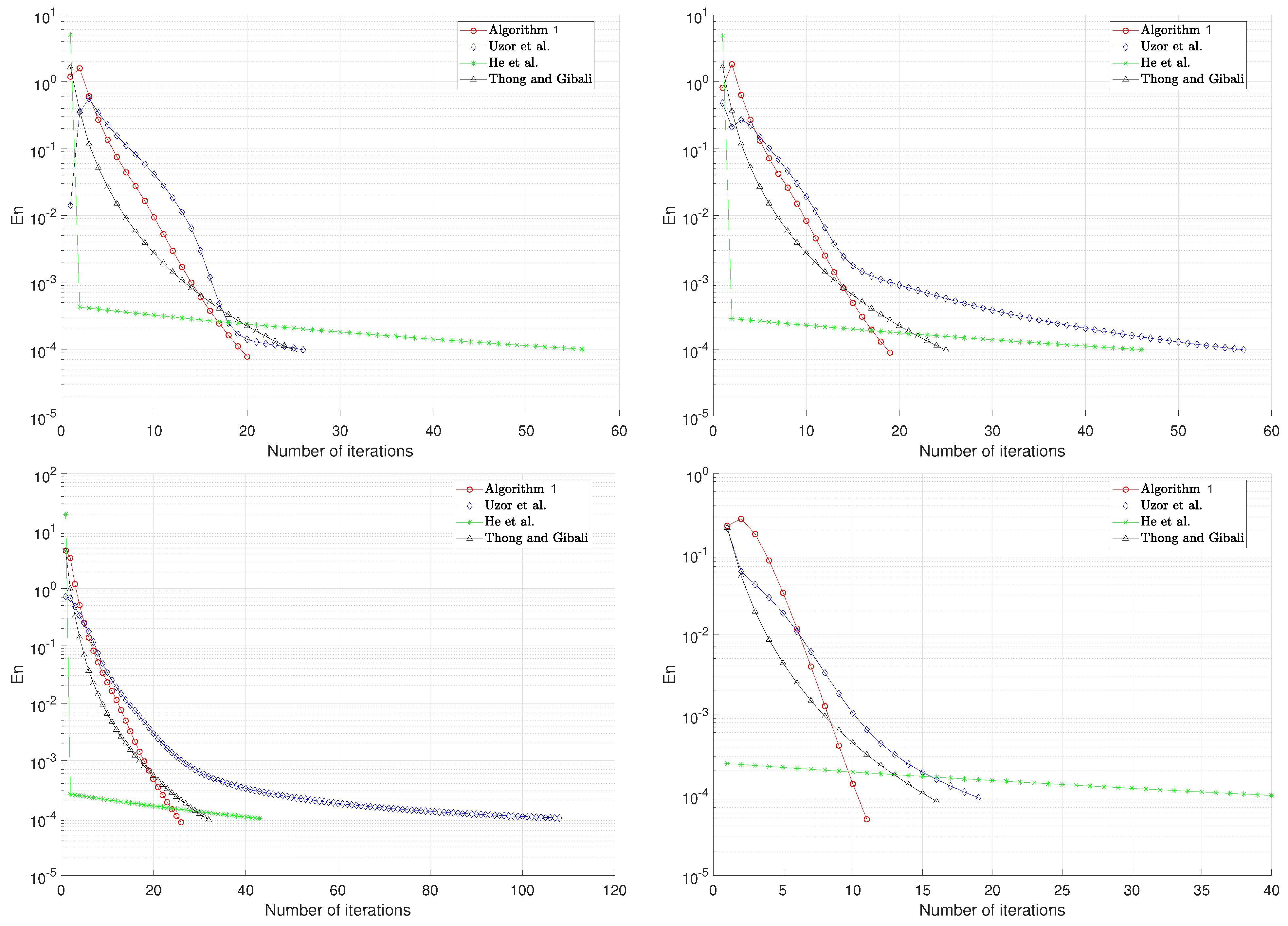
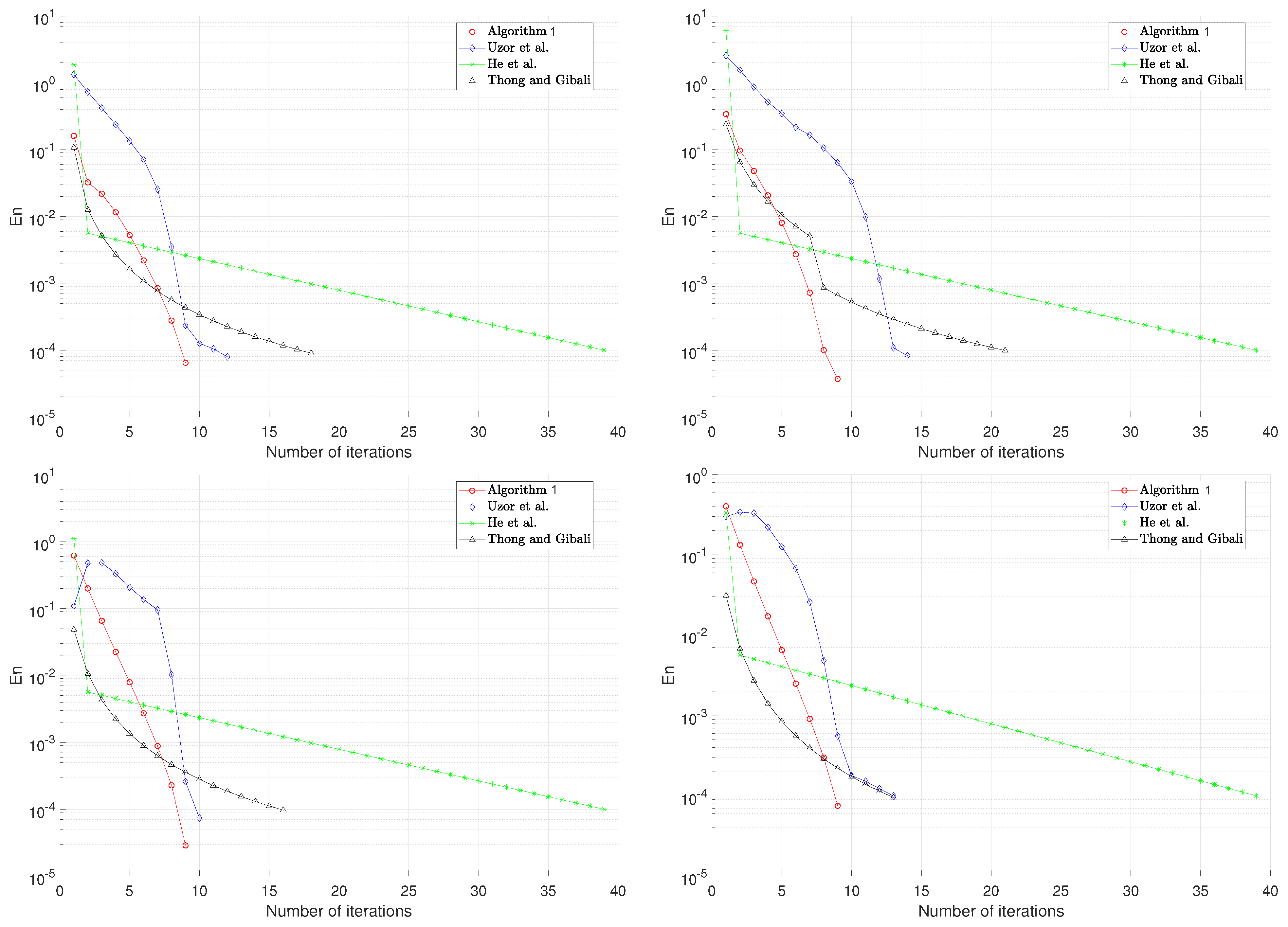
5. Numerical Example

In this section, we present two numerical examples to illustrate the behavior of the sequences generated by Algorithm 1 and make comparisons with the algorithms presented in [6,36,37]. All the programs are implemented in MATLAB 2023b on a Intel(R)Core(TM) i5-8250S CPU @1.60 GHz computer with 8.00 GB RAM.

Example 1.

Consider the variational inequality $VI(\mathcal{C},\mathcal{F})$(1) with the feasible set $C:=C^1\cap C^2\subseteq {\mathbb{R}}^2,$ where

$${\mathcal{C}}^1:=\{(a_1,a_2)\in {\mathbb{R}}^2|c_1(a_1,a_2):=a_1^2-a_2\le 0\},$$

(56)

and

$${\mathcal{C}}^2:=\{(a_1,a_2)\in {\mathbb{R}}^2|c_2(a_1,a_2):=a_1^2+a_2^2-2\le 0\},$$

(57)

and $\mathcal{F}:{\mathbb{R}}^2\to {\mathbb{R}}^2$ is defined by $\mathcal{F}(a_1,a_2)=(3h\left(a_1\right),2a_1+a_2),$ where

$$\begin{array}{cc}\hfill h\left(t\right):=& \left\{\begin{array}{c}e(t-1)+e,ift>1,\hfill \\ e^t,if-1\le t\le 1,\hfill \\ e^{-1}(t+1)+e^{-1},ift<-1.\hfill \end{array}\right.\hfill \end{array}$$

(58)

We observe from Lemma 3 that the solution set of the variational inequality problem $VI(\mathcal{C},\mathcal{F})\ne 0$ and $(-1,1)$ is its solution. The following constants, which can be obtained through simple calculations, are used: Lipschitz constants of the functions $c_i^{\prime },$ for $i=1,2$ are ${\mathcal{L}}_1={\mathcal{L}}_2=2$ and thus $\mathcal{L}=max\{{\mathcal{L}}_1,{\mathcal{L}}_2\}.$ Furthermore, based on Assumption 1 (3)(iv), $M=3\sqrt{e^2+1}$ and $M^{\prime }=6\sqrt{e^2+1}.$ As in TRSSEM, $v=0.99,\sigma =1$ and $\rho :=0.04.$ To implement SEM, we first need to estimate the Lipschitz connstant of $\mathcal{F}$, which is $\sqrt{9e^2+5}$, and also calculate the projection operator $P_{{\mathcal{C}}^1\cap {\mathcal{C}}^2}.$ This operator without explicit expression is a weakness of SEM. Furthermore, control parameter conditions are taken as follows: $\theta ={\displaystyle \frac{1}{2}},{\xi }_m={\displaystyle \frac{1}{m^{1.1}}},{\varphi }_m={\displaystyle \frac{1}{2m+1}},{\alpha }_m={\displaystyle \frac{1}{m+1}},{\beta }_m={\displaystyle \frac{1}{13m+15}},\delta =0.5,{\sigma }_m={\displaystyle \frac{1}{m\sqrt{m}}},{\lambda }_1=0.97.$ The numerical and graphical results of three methods are shown in Figure 1. The different initial values of $a_0$ and $a_1$ are as follows. The process is terminated by using the stopping criterion $\parallel a_{m+1}-a_m\parallel \le ϵ,$ where $ϵ={10}^{-4}.$

(Case 1): 

$a_0=\left[2.02.0\right]$ and $a_1=\left[3.02.0\right];$

(Case 2): 

$a_0=\left[1.01.0\right]$ and $a_1=\left[2.03.0\right];$

(Case 3): 

$a_0=\left[4.02.0\right]$ and $a_1=\left[3.05.0\right];$

(Case 4): 

$a_0=\left[0.21.1\right]$ and $a_1=\left[0.71.2\right].$

The report of this example is given in Figure 1 and

Table 1. Numerical results for Example 1.

Algorithm	Case 1		Case 2		Case 3		Case 4
	Iter.	CPU Time	Iter.	CPU Time	Iter.	CPU Time	Iter.	CPU Time
Algorithm 1	20	0.0073	19	0.0065	26	0.0061	11	0.0057
He et al. [6]	57	0.0118	47	0.0129	43	0.0108	40	0.0157
Thong and Gibali [36]	25	0.0094	25	0.090	32	0.0087	16	0.0085
Uzor et al. [37]	26	0.0217	57	0.0213	108	0.0202	19	0.0089

.

Figure 1. Top left: Case 1; top right: Case 2; bottom left: Case 3; bottom right: Case 4 [6,36,37].

Figure 1. Top left: Case 1; top right: Case 2; bottom left: Case 3; bottom right: Case 4 [6,36,37].

Example 2.

Suppose $\mathcal{F}\left(a\right)=2a,\forall a\in \mathcal{H},$ and let $\mathcal{C}\subset \mathcal{H}$ be a closed, convex, and feasible set defined as follows:

$$\mathcal{C}:={\cap }_{i=1}^m{\mathcal{C}}^i:={\cap }_{i=1}^m\{a\in \mathcal{H}:c_i\left(a\right):= \parallel a_i{\parallel }^2-2\le 0\},$$

for each $i=1,\dots ,m,$ where $\mathcal{H}=(l_2{\left(\mathbb{R}\right),\parallel .\parallel ),\parallel a\parallel }_2={\left({\sum }_{k=1}^{\infty }{\left|a_k\right|}^2\right)}^{{\displaystyle \frac{1}{2}}},\langle a,b\rangle ={\sum }_{k=1}^{\infty }{a}_k{b}_k,\forall a\in l_2\left(\mathbb{R}\right),$ and $l_2\left(\mathbb{R}\right):=\left\{a=(a_1,a_2,\dots ,a_m,\dots ),a_k\in \mathbb{R}:{\sum }_{k=1}^{\infty }{\left|x_k\right|}^2<\infty \right\}.$ We choose the following as our control parameters: $\theta ={\displaystyle \frac{1}{2}},{\xi }_m={\displaystyle \frac{1}{m^{1.1}}},{\varphi }_m={\displaystyle \frac{1}{2m+1}},{\alpha }_m={\displaystyle \frac{1}{m+1}},{\beta }_m={\displaystyle \frac{1}{13m+15}},\delta =0.5,{\xi }_m={\left({\displaystyle \frac{2}{3m+1}}\right)}^2,{\lambda }_1=3.97,{\sigma }_m={\displaystyle \frac{30}{{(3m+4)}^2}}.$ The process is terminated by using the stopping criterion $\parallel a_{m+1}-a_m\parallel \le ϵ,$ where $ϵ={10}^{-4}.$ We consider the following cases for the initial points $a_0$ and $a_1;$

(Case i)

$a_0=(1.7,1.6,\cdots ,0,\cdots )$ and $a_1=(2.1,2.2,\cdots ,0,\cdots );$

(Case ii)

$a_0=(2.2,1.1,\cdots ,0,\cdots )$ and $a_1=(0.71,1.12,\cdots ,0,\cdots );$

(Case iii)

$a_0=(3.7,2.6,\cdots ,0,\cdots )$ and $a_1=(3.1,2.5,\cdots ,0,\cdots );$

(Case iv)

$a_0=(0.64,1.75,\cdots ,0,\cdots )$ and $a_1=(0.95,1.75,\cdots ,0,\cdots ).$

The report of this example is given in Figure 2.

6. Conclusions

A novel iterative method was proposed for approximating the solution of a class of variational inequality problems defined over the intersection of sub-level sets of a countable family of convex functions. The method requires only a single projection onto a half space for computation. It was shown that the sequence generated by the proposed method converges strongly to the minimum-norm solution of the problem. The efficiency and validity of the method were demonstrated through two numerical examples. In the future, we intend to study the convergence behavior of our proposed algorithm in Banach spaces under weaker conditions, as well as to develop accelerated variants that further reduce computational complexity.

References

1. Fichera, G. Sul problem elastostatico di signorini con ambigue condizioni al contorno. Atti Accad. Naz. Lincei Cl Sci. Fis. Mat. Nat. 1963, 34, 138–142. [Google Scholar]
2. Stampacchia, G. Variational Inequalities. In Theory and Applications of Monotone Operators, Proceedings of the NATO Advanced Study Institute, Venice, Italy, 17–30 June 1968; Edizioni Odersi: Gubbio, Italy, 1968; pp. 102–192. [Google Scholar]
3. Censor, Y.; Gibali, A.; Reich, S. Extensions of Korpelevich’s extragradient method for the variational inequality problem in Euclidean space. Optimization 2012, 61, 1119–1132. [Google Scholar] [CrossRef]
4. Fukushima, M. A relaxed projection method for variational inequalities. Math. Program. 1986, 35, 58–70. [Google Scholar] [CrossRef]
5. Gu, Z.; Mani, G.; Gnanaprakasam, A.J.; Li, Y. Solving a System of Nonlinear Integral Equations via Common Fixed Point Theorems on Bicomplex Partial Metric Space. Mathematics 2021, 9, 1584. [Google Scholar] [CrossRef]
6. He, S.; Yang, C. Solving the variational inequality problem defined on intersection of finite level sets. Abstr. Appl. Anal. 2013, 2013, 942315. [Google Scholar] [CrossRef]
7. Korpelevich, G.M. An extragradient method for finding saddle points and for other problems. Ekon. Mat. Metody 1976, 12, 747–756. [Google Scholar]
8. Nallaselli, G.; Baazeem, A.S.; Gnanaprakasam, A.J.; Mani, G.; Javed, K.; Ameer, E.; Mlaiki, N. Fixed Point Theorems via Orthogonal Convex Contraction in Orthogonal b-Metric Spaces and Applications. Axioms 2023, 12, 143. [Google Scholar] [CrossRef]
9. Beg, I.; Mani, G.; Gnanaprakasam, A.J. Best proximity point of generalized F-proximal non-self contractions. J. Fixed Point Theory Appl. 2021, 23, 49. [Google Scholar] [CrossRef]
10. Gnanaprakasam, A.J.; Nallaselli, G.; Haq, A.U.; Mani, G.; Baloch, I.A.; Nonlaopon, K. Common Fixed-Points Technique for the Existence of a Solution to Fractional Integro-Differential Equations via Orthogonal Branciari Metric Spaces. Symmetry 2022, 14, 1859. [Google Scholar] [CrossRef]
11. Ramaswamy, R.; Mani, G.; Gnanaprakasam, A.J.; Abdelnaby, O.A.A.; Stojiljković, V.; Radojevic, S.; Radenović, S. Fixed Points on Covariant and Contravariant Maps with an Application. Mathematics 2022, 10, 4385. [Google Scholar] [CrossRef]
12. Alakoya, T.O.; Taiwo, A.; Mewomo, O.T.; Cho, Y.J. An iterative algorithm for solving variational inequality generalized mixed equilibrium, convex minimization and zeros problems for a class of nonexpansive-type mappings. Ann. Univ. Ferrara Sez. VII Sci. Mat. 2021, 67, 1–31. [Google Scholar] [CrossRef]
13. Dong, Q.L.; Cho, Y.J.; Zhong, L.L.; Rassias, T.M. Inertial projection and contraction algorithms for variational inequalities. J. Glob. Optim. 2017, 70, 687–704. [Google Scholar] [CrossRef]
14. He, S.; Dong, Q.-L.; Tian, H. Relaxed projection and contraction methods for solving Lipschitz-continuous monotone variational inequalities. Rev. De La Real Acad. De Cienc. Exactas Fis. Y Nat. Ser. A Mat. 2019, 113, 2773–2791. [Google Scholar] [CrossRef]
15. Ogwo, G.N.; Izuchukwu, C.; Mewomo, O.T. A modified extragradient algorithm for a certain class of split pseudo-monotone variational inequality problem. Numer. Algebra Control Optim. 2022, 12, 373–393. [Google Scholar] [CrossRef]
16. Ceng, L.; Petrușel, A.; Qin, X.; Yao, J. A modified inertial subgradient extragradient method for solving pseudomonotone variational inequalities and common fixed point problems. Fixed Point Theory 2020, 21, 93–108. [Google Scholar] [CrossRef]
17. Iusem, A.N.; Nasri, M. Korpelevich’s method for variational inequality problems in Banach spaces. J. Glob. Optim. 2011, 50, 59–76. [Google Scholar] [CrossRef]
18. Ogwo, G.N.; Izuchukwu, C.; Mewomo, O.T. Inertial methods for finding minimum-norm solutions of the split variational inequality problem beyond monotonicity. Numer. Algorithms 2021, 88, 1419–1456. [Google Scholar] [CrossRef]
19. Tseng, P. A Modified forward-backward splitting method for maximal monotone mappings. SIAM J. Control Optim. 2000, 38, 431–446. [Google Scholar] [CrossRef]
20. Yang, J.; Liu, H. Strong convergence result for solving monotone variational inequalities in Hilbert space. Numer. Algorithms 2019, 80, 741–752. [Google Scholar] [CrossRef]
21. Censor, Y.; Gibali, A.; Reich, S. The Split Variational Inequality Problem; The Technion-Israel Institute of Technology: Haifa, Israel, 2010. [Google Scholar]
22. He, S. A class of projection and contraction methods for monotone variational inequalities. Appl. Math. Optim. 1997, 35, 69–76. [Google Scholar] [CrossRef]
23. He, B.; Yuan, X.; Zhang, J.J. Comparison of two kinds of prediction-correction methods for monotone variational inequalities. Comput. Optim. Appl. 2004, 27, 247–267. [Google Scholar] [CrossRef]
24. Solodov, M.V.; Tseng, P. Modified projection-type methods for monotone variational inequalities. SIAM J. Control Optim. 1996, 34, 1814–1830. [Google Scholar] [CrossRef]
25. Sun, D. A class of iterative methods for solving nonlinear projection equations. J. Optim. Theory Appl. 1996, 91, 123–140. [Google Scholar] [CrossRef]
26. Polyak, B. Some methods of speeding up the convergence of iteration methods. USSR Comput. Math. Math. Phys. 1964, 4, 1–17. [Google Scholar] [CrossRef]
27. Cao, Y.; Guo, K. On the convergence of inertial two-subgradient extragradient method for solving variational inequality problems. Optimization 2020, 69, 1237–1253. [Google Scholar] [CrossRef]
28. Alvarez, F. Weak convergence of a relaxed and inertial hybrid projection-proximal point algorithm for maximal monotone operators in hilbert space. SIAM J. Optim. 2004, 14, 773–782. [Google Scholar] [CrossRef]
29. Attouch, H.; Cabot, A. Convergence of a relaxed inertial forward–backward algorithm for structured monotone inclusions. Appl. Math. Optim. 2019, 80, 547–598. [Google Scholar] [CrossRef]
30. Iutzeler, F.; Hendrickx, J.M. A generic online acceleration scheme for optimization algorithms via relaxation and inertia. Optim. Methods Softw. 2019, 34, 383–405. [Google Scholar] [CrossRef]
31. He, S.; Wu, T.; Gibali, A.; Dong, Q.-L. Totally relaxed, self-adaptive algorithm for solving variational inequalities over the intersection of sub-level sets. Optimization 2018, 67, 1487–1504. [Google Scholar] [CrossRef]
32. Bauschke, H.H.; Combettes, P.L. Convex Analysis and Monotone Operator Theory in Hilbert Spaces, 2nd ed.; Springer: New York, NY, USA, 2017. [Google Scholar]
33. Nguyen, H.Q.; Xu, H.K. The supporting hyperplane and an alternative to solutions of variational inequalities. J. Nonlinear Convex Anal. 2015, 16, 2323–2331. [Google Scholar]
34. Saejung, S.; Yotkaew, P. Approximation of zeros of inverse strongly monotone operators in Banach spaces. Nonlinear Anal. Theory Methods Appl. 2012, 75, 742–750. [Google Scholar] [CrossRef]
35. Tan, K.K.; Xu, H.K. Approximating Fixed Points of Nonexpansive Mappings by the Ishikawa Iteration Process. J. Math. Anal. Appl. 1993, 178, 301–308. [Google Scholar] [CrossRef]
36. Thong, D.V.; Gibali, A. Two strong convergence subgradient extragradient methods for solving variational inequalities in Hilbert spaces. Jpn. J. Ind. Appl. Math. 2019, 36, 299–321. [Google Scholar] [CrossRef]
37. Uzor, V.A.; Mewomo, O.T.; Alakoya, T.O.; Gibali, A. Outer approximated projection and contraction method for solving variational inequalities. J. Inequalities Appl. 2023, 2023, 141. [Google Scholar] [CrossRef]
Figure 2. Top left: Case i; top right: Case ii; bottom left: Case iii; bottom right: Case iv [6,36,37].
Axioms 14 00354 g002