1. Introduction
Orthonormal frames are essential tools for studying the differential geometry of curves and surfaces [
1,
2,
3]. The Frenet–Serret frame of a space curve and the Darboux frame of a surface curve are among the most well-known of these frames [
4,
5,
6]. More general frames along space curves or surface curves have been introduced by Myller. He defined a configuration in
, known as the Myller configuration
, by considering a unit vector field
and a plane
along a curve
C, referring to them as a versor field
and a plane field
, respectively, with the condition that
. When the planes
are tangent to
C, this configuration becomes a special case called the tangent Myller configuration, denoted by
. Specifically, if the curve
C is a surface curve lying on a surface
with arclength parameter
s,
serves as the tangent versor field to
S along
C, and
is the tangent plane field to
S along
In this context,
is referred to as the tangent Myller configuration intrinsically associated with the geometric objects
and
. Thus, the geometry of the versor field
on a surface
S corresponds to the geometry of the associated Myller configurations
, which in turn represents a particular case of
. In the special instance where the tangent Myller configuration
is the associated Myller configuration to a curve
C on a surface
we obtain the classical theory of surface curves (curves lying on a surface).
Myller studied the parallelism of versor field
in the plane field
[
7]. He obtained a generalization of the parallelism of Levi-Civita on the curved surfaces. Later, Mayer introduced some new invariants for
and
[
8]. Miron extended the notion of Myller configuration in Riemannian geometry [
9]. Vaisman considered the Myller configuration in the symplectic geometry [
10]. Furthermore, Myller configuration has been studied in different spaces [
11,
12,
13]. Macsim, Mihai, and Olteanu have investigated rectifying-type curves in a Myller configuration [
14]. Recently, the authors defined some special helices in
M and provided the characterizations for those curves [
15]. In recent years, several works have further expanded the study of geometric structures in Euclidean spaces, such as the study of sweeping surfaces and directional developable surfaces [
16,
17,
18]. Li and other researchers also explored osculating curves [
19,
20,
21] and generalized Bertrand curve pairs [
22,
23,
24]. These works contribute to a deeper understanding of geometric curves in higher-dimensional spaces and offer a broader context for our exploration of slant helices and Darboux helices in the Myller configuration
M [
25,
26,
27].
In the present paper, we study slant helices and Darboux helices in the Myller configuration M. We provide characterizations and axes for these curves. Moreover, we introduce the alternative frame of a curve C in M and present the geometric interpretations of alternative invariants of C. Finally, we obtain the differential equations related to curves, helices, and slant helices in M.
2. Preliminaries
In this section, a brief summary of curves in Myller configuration
are introduced. For more detailed information, we refer to [
9].
Let
be a versor field and
be a plane field such that
in
. The pair
is called Myller configuration in
and is denoted by
or, briefly,
M. Let
denotes an orthonormal frame. Then,
can be expressed in the form
where
is the position vector of
C,
s is the arclength parameter of
and
Writing
and considering
one can define versor field
as follows:
where
is called the curvature (or
-curvature) of
. The versor field
is orthogonal to
and exists when
. By defining the versor field
an orthonormal and positively oriented frame is obtained. This frame is called the invariant frame of Frenet type for the versor field
and denoted by
or, briefly,
[
9].
The derivative formulas for
are
with
and
where
is called the torsion (or
-torsion) of
The curvatures
and
have the same geometrical interpretation as the curvature and torsion of a curve in
, and the functions
,
are invariants of the versor field
[
9]. If
, one obtains the Frenet equations of a curve in
The following theorem serves as the fundamental theorem for the versor field :
Theorem 1 ([
9])
. If the functions , and , of class and are given a priori, for , then there exists a curve with arclength s and a versor field , such that the functions , and are the invariants of . Any two such versor fields differ by a proper Euclidean motion. We give the definition of -helix ( as follows.
Definition 1 ([
15])
. Let the curve C with the invariant type Frenet frame in M be a helix in with the unit axis , that is, is constant. Then, the curve C is called -helix if the versor field makes a constant angle with the same fixed direction , where . 3. Slant Helices in Myller Configuration
In this section, we focus on slant helices (or -helices) in the Myller configuration We provide characterizations for slant helices in this context. Specifically, we explore the geometric properties and conditions that define a curve as a slant helix in the Myller configuration, analyzing its behavior and relationships with other curve types, and we give the characterizations for slant helix in M.
Definition 2. Let the curve C with the invariant-type Frenet frame in M be a helix in with the unit axis , that is, is constant. The curve C is called a slant helix(or -helix) in M if the versor field makes a constant angle with the same fixed unit direction
Theorem 2. The curve C in M with Frenet frame and is a slant helix iff the following functions are constant: Proof. From Definition 2, there exists a constant angle
such that
Then, for the axis
, we can write
where
and
are smooth functions of
s. Since
is constant, differentiating (
4) with respect to
s yields
and we have the system
From the second equation in (
5), it follows that
. Substituting this into the first and third equations in (
5) gives the differential equation
Considering the transformation
the differential equation given in (
6) becomes
, which has the solution
, where
is the integration constant. Hence,
. Since
, from (
4), we have
Then, (
4) becomes
From the third equation in (
5), it follows that
Hence, we have that
is a constant function. Also, from Definition 2, it follows that
is constant.
Conversely, let the functions
and
given in (
2) be constants and
be a unit vector defined by
where
is constant. Differentiating the last equality gives
Now, substituting (
2) in this result, we have
, i.e.,
is a constant vector field and, since
and
are constants, we obtain that
C is a slant helix in Myller configuration
□
From Theorem 2, the following corollary is obtained.
Corollary 1. The axis of slant helix C in the Myller configuration M is given bywhere θ is the constant angle defined by 4. Darboux Helices in Myller Configuration (,,)
The alternative frame of a curve is a useful tool to study the properties of the curve in the Euclidean 3-space. This frame is obtained from the Frenet frame of the curve and provides advantages in characterizing certain special curves and surfaces [
28,
29,
30,
31]. In this section, we first define the alternative frame of a curve
C and provide the geometric interpretations of the alternative curvatures. Next, we define Darboux helices in
M and characterize these helices by means of an alternative frame.
Let be a versor field with invariant-type Frenet frame in the Myller configuration M. The vector is called the Darboux vector field of the Frenet frame .
Let us define
and
. Then,
=
is an othonormal frame of the versor field
in
M called the alternative Frenet frame (or AF-frame) of
. The moving equations of the AF-frame are as follows:
with
and
where
and
are invariants and called the alternative curvatures of versor field
.
The geometric interpretations of the functions
can be expressed as follows:
For the geometric interpretations of the invariants we present the following theorem.
Theorem 3. Let us consider a variation of an alternative frame
And let be the oriented angle between the successive versor fields and be the oriented angle between the successive versor fields . Alternative curvatures p and q of the versor field are given byrespectively. Proof. Let
be the oriented angle between the successive versor fields
. Then, the angle function between versor fields
and
is defined by
. From (
9), we have
. Then, we can write
Considering the cosine theorem, we have
Since
and
are unit, (
12) becomes
By using trigonometric relation
the last equality gives
. Hence,
Then, from (
11), we have
. The proof of second equality in (
10) can be provided in a similar manner. □
Theorem 4. Let be a versor field with curvatures and alternative curvatures p and q. The relationship between these curvatures are given as follows: Proof. Let define the function
Thus, the alternative curvature
q takes the form
. Integrating the last equality gives
. Hence, we obtain
. Considering the relation
and trigonometric relations, we obtained Equalities (
13). Now, comparing (
1) and (
8) and using (
13), we have Equalities (
14) □
Definition 3. Let the curve C with the invariant-type Frenet frame in M be a helix in with the unit axis , that is, is constant. Let denote the AF-frame of C in the Myller configuration M. The curve C is called a Darboux helix in M if the versor field makes a constant angle with the constant versor field
Theorem 5. The curve C with AF-frame and in M is a Darboux helix if and only if the following functions are constant: Proof. Let
C be a Darboux helix in
M. Then, there exists a constant angle
such that
Differentiating the last equality with respect to
s and considering (
9), we obtain
. Hence, we have
. Now, we can write
. Since
is a constant versor field, the differentiation of the last equality yields
Hence, we have that
is constant. Furthermore, since
by considering (
13) and (
14), we have
which finishes the proof. □
From Theorem 5, the following corollaries are obtained.
Corollary 2. The curve C in M is a Darboux helix if and only if C is a slant helix.
Corollary 3. The axis of a Darboux helix C in terms of Frenet frame is given by 5. Differential Equations Characterizing Slant Helices and Darboux
Helices in
In this section, we present general differential equations for a versor field in M with respect to both AF-frame and the Frenet-type frame . Furthermore, we derive differential equations that characterize helices, slant helices, and Darboux helices in M.
Theorem 6. Let be a versor field with AF-frame and non-zero alternative curvatures p and q. The versor field satisfies the following differential equation: Proof. From the second equation in (
9), it follows that
and, from the first equation in (
9), we obtain
. Considering the last equality and third equation in (
9), we obtain
Differentiating
, we have
Writing (
19) in (
17) gives
By differentiating the last equality and taking into account (
18), we have (
16). □
Corollary 4. The curve C with AF-frame and non-zero curvatures is a slant helix (or Darboux helix) iff is constant and the versor field satisfies the following differential equation: Proof. From Theorem 5, we have that the curve
C is a slant helix (or Darboux helix) if and only if
and
g are constants. By applying this to (
16), (
20) is obtained. □
Theorem 7. Let be a versor field with AF-frame and non-zero alternative curvatures . The versor field satisfies the following differential equation:where , and Proof. From the second equality in (
9), we have
Differentiating (
21) and considering the first and third equalities in (
9), it follows that
Writing (
22) in (
21), we have
Now, differentiating (
23), we obtain the desired equation. □
Corollary 5. The curve C with AF-frame and non-zero curvatures is a slant helix (or Darboux helix) iff is constant and the versor field satisfies the following differential equation Proof. From the second equality in (
9), it follows
and differentiating that gives
By taking into account the first and third equations in (
9), the last equality becomes
From (
25),
C is a slant helix (or Darboux helix) if and only if
holds. □
Theorem 8. Let be a versor field with AF-frame and non-zero alternative curvatures . The versor field satisfies the following differential equation: Proof. From the third equation in (9), we obtain
, and differentiating this gives
Writing that in the second equation in (
9), it follows that
Differentiating the last equality gives
Writing
in the first equation in (
9), we have
. Considering this in (
27), we have (
26). □
Corollary 6. The curve C with AF-frame and non-zero curvatures is a slant helix (or Darboux helix) iff is constant and the versor field satisfies the following differential equation: Proof. The proof can be clearly established based on the assertions made in Theorem 9. □
In Theorem 6, we present the differential equation of a curve C in M with respect to versor field In the following theorems, we provide the differential equations of a curve C in M with respect to versor fields and The proofs of these theorems can be derived in a manner similar to that described above.
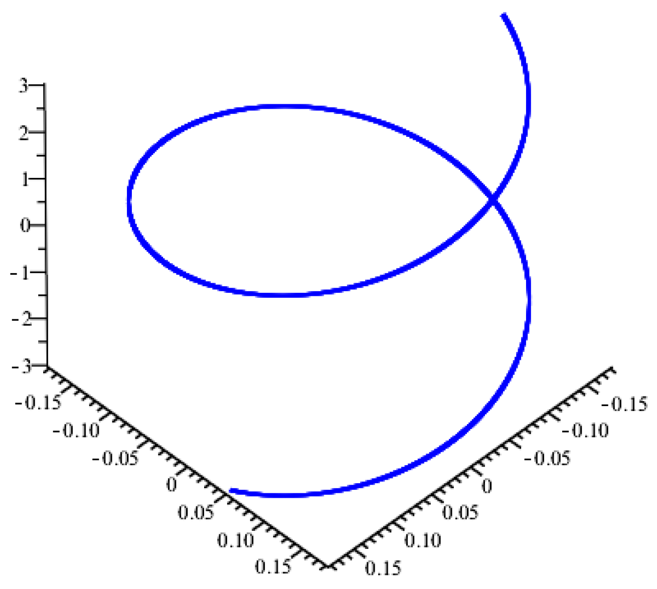
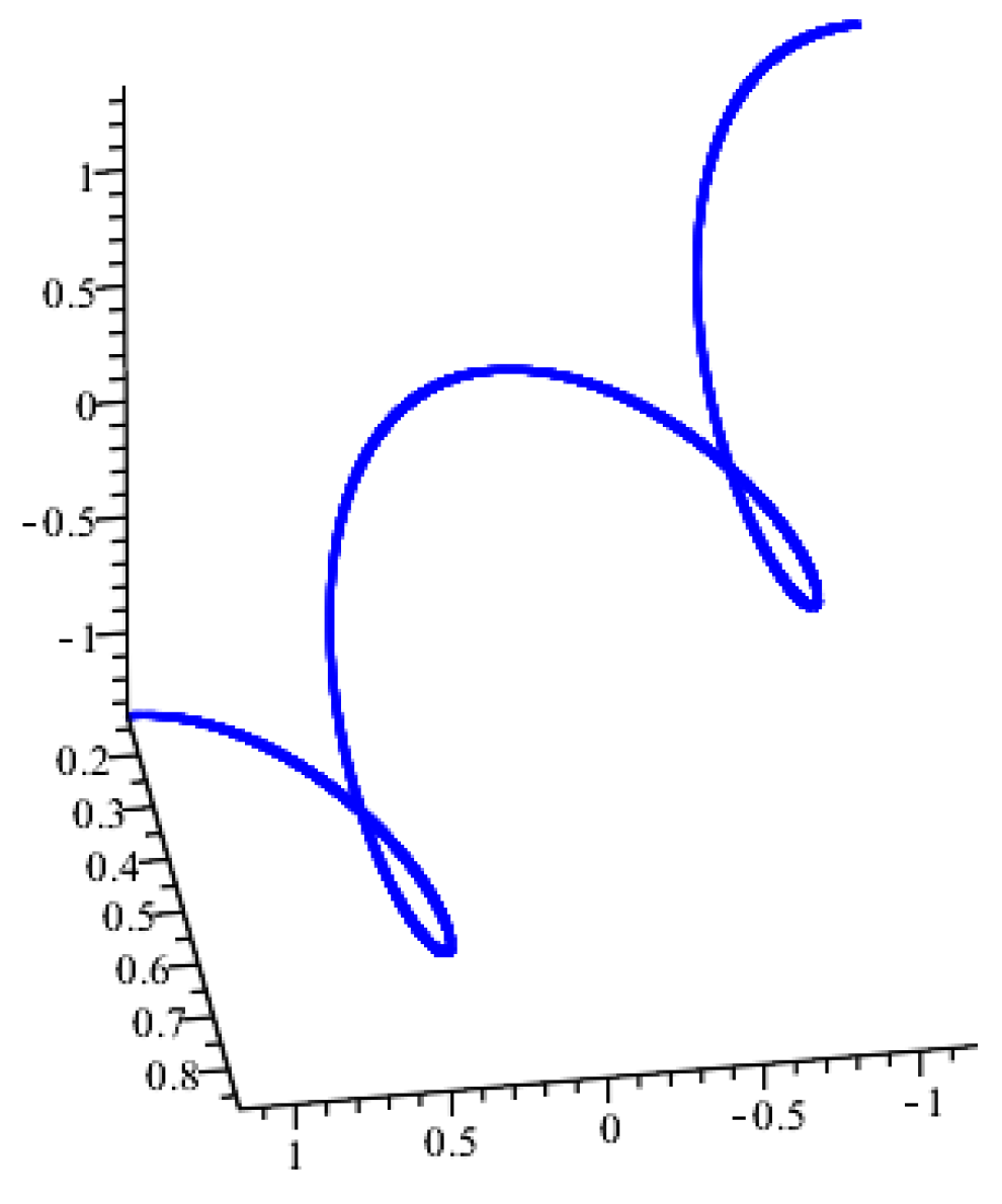
Theorem 9. The versor field of the versor field with Frenet frame and non-zero curvatures satisfies the following differential equation: Theorem 10. The versor field of the versor field with Frenet frame and non-zero curvatures satisfies the following differential equation:where and Theorem 11. The versor field of the versor field with Frenet frame and non-zero curvatures satisfies the following differential equation: Example 1. Let us consider the versor fields The curvatures and are computed as which gives Then, we have . This results in or By choosing , and we obtain i.e., σ and ρ are constants. Then, the curve given by the parametric form is a slant helix in M (Figure 1). If we choose , and it follows that , meaning that both σ and ρ are constants. Consequently, the curve given by the parametrization is a slant helix in M (Figure 2). Both curves and are also Darboux helices in M and they satisfy the differential Equations (20), (24) and (28). Example 2. Let us consider the versor fields The curvatures and are computed as which gives Then, we have . This results in or By choosing , and we obtain i.e., σ and ρ are constants. Then, the curve given by the parametric formis a slant helix in M (Figure 3). If we choose , and it follows that , meaning that both σ and ρ are constants. Consequently, the curve given by the parametrizationis a slant helix in M (Figure 4). Both curves and are also Darboux helices in M and they satisfy the differential Equations (20), (24) and (28). 6. Conclusions
Slant helices and Darboux helices in the Myller configuration M are introduced and studied. It is shown that a curve C in M is a slant helix if and only if it is also a Darboux helix in M. Moreover, the alternative frame of a curve C in M is introduced, and geometric interpretations of alternative curvatures are provided. Subsequently, general differential equations for a curve C in M are derived with respect to both the alternative frame and the Frenet-type frame . Finally, differential equations characterizing helices, slant helices, and Darboux helices in M are presented.
Author Contributions
Conceptualization, Y.L., A.A., M.Ö., and Y.X.; methodology, Y.L., A.A., M.Ö., and Y.X.; investigation, Y.L., A.A., M.Ö., and Y.X.; writing—original draft preparation, Y.L., A.A., M.Ö., and Y.X.; writing—review and editing, Y.L., A.A., M.Ö., and Y.X. All authors have read and agreed to the published version of the manuscript.
Funding
This research received no external funding.
Data Availability Statement
Data are contained within the article.
Conflicts of Interest
The authors declare no conflicts of interest.
References
- Stoker, J.J. Differential Geometry, Pure and Applied Mathematics; John Wiley&Sons: Hoboken, NJ, USA, 2011; Volume 20, p. 62. [Google Scholar]
- Struik, D.J. Lectures on Classical Differential Geometry, 2nd ed.; Addison Wesley: Dover, UK, 1988. [Google Scholar]
- Izumiya, S.; Romero Fuster, M.C.; Ruas, M.A.S.; Tari, F. Differential Geometry from a Singularity Theory Viewpoint; World Scientific Publishing Co. Pte. Ltd.: Hackensack, NJ, USA, 2016. [Google Scholar]
- Izumiya, S.; Takeuchi, N. Special curves and ruled surfaces. BeiträGe Algebra Geom. 2003, 44, 203–212. [Google Scholar]
- Izumiya, S.; Takeuchi, N. New special curves and developable surfaces. Turk J. Math. 2004, 28, 153–163. [Google Scholar]
- Hananoi, S.; Izumiya, S. Normal developable surfaces of surfaces along curves. Proc. R. Soc. Edinb. Sect. Math. 2017, 147, 177–203. [Google Scholar] [CrossRef]
- Myller, A.I. Quelques prorietes des surfaces reglees en liaison avec la theorie du parallelisme de Levi-Civita. C.R. Paris 1922, 174, 997. [Google Scholar]
- Mayer, O. Etude sur les Reseaux de M. Myller; Annales scientifiques de l’Université de Jassy: Jassy, Romania, 1926; Volume XIV. [Google Scholar]
- Miron, R. The Geometry of Myller Configuration. Applications to Theory of Surfaces and Nonholonomic Manifolds; Romanian Academy: Bucharest, Romania, 2010. [Google Scholar]
- Vaisman, I. Simplectic Geometry and Secondary Characteristic Closses; Progress in Mathematics, 72; Birkhauser Verlag: Basel, Switzerland, 1994. [Google Scholar]
- Constantinescu, O. Myller configurations in Finsler spaces. Applications to the study of subspaces and of torse forming vector fields. J. Korean Math. Soc. 2008, 45, 1443–1482. [Google Scholar] [CrossRef]
- Constantinescu, O. Myller configurations in Finsler spaces. Differ.-Geom.-Dyn. Syst. 2006, 8, 69–76. [Google Scholar]
- İşbilir, Z.; Doğan Yazıcı, B.; Tosun, M. On special curves in Lie groups with Myller configuration. Mathematical Methods in the Applied Sciences. Math. Methods Appl. Sci. 2004, 47, 11693–11708. [Google Scholar] [CrossRef]
- Macsim, G.; Mihai, A.; Olteanu, A. On rectifying type curves in a Myller configuration. Bull. Korean Math. Soc. 2019, 56, 383–390. [Google Scholar] [CrossRef]
- Alkan, A.; Önder, M. Some special helices in Myller configuration. Appl. Math.E -Notes 2023, in press. [Google Scholar]
- Li, Y.; Eren, K.; Ersoy, S.; Savic, A. Modified Sweeping Surfaces in Euclidean 3-Space. Axioms 2024, 13, 800. [Google Scholar] [CrossRef]
- Zhu, M.; Yang, H.; Li, Y.; Abdel-Baky, R.A.; AL-Jedani, A.; Khalifa, M. Directional developable surfaces and their singularities in Euclidean 3-space. Filomat 2024, 38, 11333–11347. [Google Scholar]
- Zhu, Y.; Li, Y.; Eren, K.; Ersoy, S. Sweeping Surfaces of Polynomial Curves in Euclidean 3-space. An. St. Univ. Ovidius Constanta 2025, 33, 293–311. [Google Scholar]
- Cheng, Y.; Li, Y.; Badyal, P.; Singh, K.; Sharma, S. Conformal Interactions of Osculating Curves on Regular Surfaces in Euclidean 3-Space. Mathematics 2025, 13, 881. [Google Scholar] [CrossRef]
- Ilarslan, K.; Kilic, N.; Erdem, H.A. Osculating curves in 4-dimensional semi-Euclidean space with index 2. Open Math. 2017, 15, 562–567. [Google Scholar] [CrossRef]
- Ilarslan, K.; Nešović, E. Some characterizations of pseudo and partially null osculating curves in Minkowski space-time. Int. Electron. J. Geom. 2011, 4, 1–12. [Google Scholar]
- Li, Y.; Kecilioglu, O.; Ilarslan, K. Generalized Bertrand Curve Pairs in Euclidean Four- Dimensional Space. Axioms 2025, 14, 253. [Google Scholar] [CrossRef]
- Camci, C.; Ucum, A.; Ilarslan, K. A new approach to Bertrand curves in Euclidean 3-space. J. Geom. 2020, 111, 49. [Google Scholar] [CrossRef]
- Ucum, A.; Ilarslan, K. On timelike Bertrand curves in Minkowski 3-space. Honam Math. J. 2016, 38, 467–477. [Google Scholar] [CrossRef]
- Macit, N.; Düldül, M. Relatively normal-slant helices lying on a surface and their characterizations. Hacet. J. Math. Stat. 2017, 46, 397–408. [Google Scholar] [CrossRef]
- Puig-Pey, J.; Gálvez, A.; Iglesias, A. Helical curves on surfaces for computer-aided geometric design and manufacturing. In Computational Science and Its Applications-ICCSA Part II; Lecture Notes in Computer Science; Springer: Berlin\Heidelberg, Germany, 2004; Volume 3044, pp. 771–778. [Google Scholar]
- Zıplar, E.; Şenol, A.; Yaylı, Y. On Darboux helices in Euclidean 3-space. Glob. J. Sci. Front. Res. Decis. Sci. 2012, 12, 73–80. [Google Scholar]
- Kula, L.; Ekmekci, N.; Yayli, Y.; Ilarslan, K. Characterizations of slant helices in Euclidean 3-space. Turk. J. Math. 2010, 34, 261–274. [Google Scholar] [CrossRef]
- Camci, Ç.; Chen, B.Y.; İlarslan, K.; Uçum, A. Sequential natural mates of Frenet curves in Euclidean 3-space. J. Geom. 2021, 112, 1–15. [Google Scholar] [CrossRef]
- Şahiner, B. Ruled surfaces according to alternative moving frame. arXiv 2019, arXiv:1910.06589. [Google Scholar]
- Uzunoğlu, B.; Gök, İ.; Yaylı, Y. A new approach on curves of constant precession. Appl. Math. Comput. 2016, 275, 317–323. [Google Scholar] [CrossRef]
| Disclaimer/Publisher’s Note: The statements, opinions and data contained in all publications are solely those of the individual author(s) and contributor(s) and not of MDPI and/or the editor(s). MDPI and/or the editor(s) disclaim responsibility for any injury to people or property resulting from any ideas, methods, instructions or products referred to in the content. |
© 2025 by the authors. Licensee MDPI, Basel, Switzerland. This article is an open access article distributed under the terms and conditions of the Creative Commons Attribution (CC BY) license (https://creativecommons.org/licenses/by/4.0/).


