Evolutionary Search for Polynomial Lyapunov Functions: A Genetic Programming Method for Exponential Stability Certification

Abstract

This paper presents a method for constructing polynomial Lyapunov functions to analyze the stability of nonlinear dynamical systems. The approach is based on genetic programming, a variant of genetic algorithms where the search space consists of hierarchical tree structures. In our formulation, these polynomial functions are represented as binary trees. The Lyapunov conditions for exponential stability are interpreted as a minimax optimization problem, using a carefully designed fitness metric to ensure positivity and dissipation within a chosen domain. The genetic algorithm then evolves candidate polynomial trees, minimizing constraint violations and continuously refining stability guarantees. Numerical examples illustrate that this methodology can effectively identify and optimize Lyapunov functions for a wide range of systems, indicating a promising direction for automated stability proofs in engineering applications.

1. Introduction

Lyapunov functions are fundamental tools for analyzing the stability of nonlinear systems [1,2,3] based on energy-based reasoning. If a system consistently dissipates energy everywhere except at the origin, it must eventually converge to the equilibrium point. Consequently, a Lyapunov function—serving as an energy-like measure—must be strictly positive definite for all states. This principle extends naturally to general nonlinear systems. Lyapunov’s direct method involves constructing a scalar function representing the system’s dynamics and analyzing its evolution over time. However, identifying such a function remains a significant challenge. Importantly, failing to find a Lyapunov function does not imply that the system is unstable, adding complexity to the task.

Numerous classical methods for identifying or approximating Lyapunov functions have been proposed, including the variable gradient method, Krasovskii’s method, and basis-function linearization; see [1,2,3,4,5,6] for a comprehensive overview. However, no universal technique exists, and constructing a Lyapunov function is generally as difficult as solving the system itself. In recent decades, advances in computational power have spurred research into numerical approaches such as sum-of-squares polynomials [7,8], piecewise affine functions [9], formal synthesis via satisfiability modulo theories (SMT) [10], and deep neural networks [11]. An in-depth survey of these methods can be found in [12], and studies on the stability of evolutionary systems are presented in [13,14].

This work introduces a numerical method for synthesizing polynomial Lyapunov functions tailored to exponentially stable dynamical systems utilizing the genetic programming (GP) paradigm [15]. GP is an evolutionary computation technique, an extension of genetic algorithms [16], which operates directly on symbolic expressions, enabling the automatic discovery and optimization of mathematical formulas. A key advantage of this approach is its ability to generate interpretable, symbolic representations of Lyapunov functions, facilitating further analysis of system dynamics.

Several prior works have explored related methodologies. Grosman and Lewin [17] applied GP techniques to the analysis of asymptotic stability. McGough et al. [18] utilized Grammatical Evolution, a specialized variant of GP. Feng et al. [19] combined deep neural networks with symbolic regression to synthesize Lyapunov functions; additional insights are provided in [20].

While these methods have demonstrated significant progress, many lack rigorous mathematical guarantees or general-purpose construction procedures. Our contributions address this gap by establishing existence criteria for polynomial Lyapunov functions in exponentially stable systems and developing a robust algorithm for their automated synthesis. The proposed method was validated across multiple benchmark systems, demonstrating its strong performance and high accuracy.

2. Exponential Stability of Dynamical Systems

In this section, we recall several fundamental concepts of exponential stability in dynamical systems. For additional details, we refer the reader to [1,2,3].

We consider an autonomous system of ordinary differential equations of the form

$$\dot{x}\left(t\right)=f\left(x\left(t\right)\right)$$

(1)

where $f:D\to {\mathbb{R}}^n$ is a locally Lipschitz continuous map defined on a domain $D\subseteq {\mathbb{R}}^n$.

We analyzed an exponentially stable equilibrium according to the following definition.

Definition 1. 

The equilibrium point $x = 0$ of (1) is exponentially stable if there exist positive constants $c$, $k$, and $\lambda$ such that

$$‖x\left(t\right)‖\le k{‖x\left(t_0\right)‖}^{-\lambda \left(t-t_0\right)}, \forall ‖x\left(t_0\right)‖<c$$

and globally exponentially stable if satisfied for any initial state $x\left(t_0\right).$

The classical Lyapunov theorem states that if one can find a continuously differentiable function $V\left(x\right):D\to \mathbb{R}$ that satisfies specified bounding conditions, then the equilibrium at the origin is exponentially stable.

Theorem 1 

(Khalil [2]). Let $x = 0$ be an equilibrium point for the nonlinear system

$$\dot{x}=f\left(t,x\right)$$

where $f:\left[0,\infty \right)\times D\to {\mathbb{R}}^n$ is piecewise continuous in $t$ and locally Lipschitz in $x$ on $\left[0,\infty \right)\times D$ and $D\subset {\mathbb{R}}^n$ is a domain that contains the origin $x=0$. Let $V\left(x\right):\left[0,\infty \right)\times D\to \mathbb{R}$ be a continuously differentiable function such that

$$k_1{‖x‖}^{\alpha }\le V\left(t,x\right)\le k_2{‖x‖}^{\alpha },$$

$${\displaystyle \frac{\partial V}{\partial t}}+{\displaystyle \frac{\partial V}{\partial x}}f\left(t, x\right)\le {-k}_3{‖x‖}^{\alpha },$$

$\forall t\ge 0$ and $\forall x\in D$, where $k_1,k_2,k_3$, and $\alpha$ are positive constants. Then, $x=0$ is exponentially stable. If the assumption holds globally, then $x=0$ is globally exponentially stable.

For nonlinear systems, stability can also be analyzed via linearization. The following theorem relates exponential stability of the nonlinear system to the stability of its linearization using the Jacobian matrix.

Theorem 2 

(Khalil [2]). Let $x=0$ be an equilibrium point for the nonlinear system

$$\dot{x}=f\left(t,x\right)$$

where $f:\left[0,\infty \right)\times D\to {\mathbb{R}}^n$ is continuously differentiable, $D=\left\{x\in {\mathbb{R}}^n \right| {‖x‖}_2<r\}$, and the Jacobian matrix $A\left(t\right)$ is bounded and Lipschitz on $D$, uniformly in $t$.

Let

$${\left.A\left(t\right)={\displaystyle \frac{\partial f}{\partial x}}\left(t,x\right)\right|}_{x=0}.$$

Then, the origin is an exponentially stable equilibrium point for the nonlinear system if and only if it is an exponentially stable equilibrium point for the linear system

$$\dot{x}=A\left(t\right)x.$$

For the autonomous system (1), the stability of $x=0$ can be determined by the eigenvalues of the constant linearization matrix.

Definition 2. 

A squared matrix $A\in {\mathbb{R}}^{n\times n}$ is called a Hurwitz matrix if all its eigenvalues ${\lambda }_i$ satisfy

$$Re{(\lambda }_i)<0.$$

Corollary 1. 

Let $x=0$ be an equilibrium point for the autonomous nonlinear system (1), where $f\left(x\right)$ is continuously differentiable in a neighborhood of $x=0$. Let $A$ be a linearization matrix of (1). Then, $x=0$ is an exponentially stable equilibrium point for the nonlinear system if and only if $A$ is a Hurwitz matrix.

The following converse theorem presented by Peet [21] guarantees the existence of a polynomial Lyapunov function for an exponentially stable equilibrium under sufficient smoothness and boundedness conditions.

Theorem 3 

(Peet [21]). Consider the system defined by Equation (1), where $f\in C^{n+2}\left({\mathbb{R}}^n\right)$. Suppose there exist constants $\mu ,\delta ,r>0$ such that

$${‖x\left(t\right)‖}_2\le \mu {‖x\left(t_0\right)‖}_2{e}^{-\delta t}$$

for all $t\ge 0$ and ${‖x\left(t_0\right)‖}_2\le r$. Then, there exists a polynomial $v:{\mathbb{R}}^n\to \mathbb{R}$ and constants $k_1,k_2,k_3>0$ such that

$$k_1{‖x‖}_2^2\le v\left(x\right)\le k_2{‖x‖}_2^2,$$

$$\nabla v{\left(x\right)}^{T}f\left(x\right)\le {-k}_3{‖x‖}_2^2,$$

for all ${‖x\left(t\right)‖}_2\le r$.

3. Genetic Programming Method for Exponential Stability Certification

In this section, we outline our proposed method, which leverages genetic programming to compute a polynomial Lyapunov function for a given dynamical system. We provide a comprehensive explanation of the underlying theoretical principles and describe the construction process of our approach.

3.1. Existence Criterion for a Polynomial Lyapunov Function

We now present a converse Lyapunov theorem, which provides the main criterion for the applicability of the proposed method.

Theorem 4. 

Let $x=0$ be an equilibrium for the nonlinear system (1), where $f\in C^{n+2}\left(D\right)$ and $D=\left\{x\in {\mathbb{R}}^n \right| {‖x‖}_2<r\}.$ Let linearization matrix $A$ of the system (1) be a Hurwitz matrix. Then, there exists a polynomial $v:{\mathbb{R}}^n\to \mathbb{R}$ and constants $k_1,k_2,k_3>0$ such that

$$k_1{‖x‖}_2^2\le v\left(x\right)\le k_2{‖x‖}_2^2,$$

$$\nabla v{\left(x\right)}^{T}f\left(x\right)\le {-k}_3{‖x‖}_2^2,$$

for all $x\in D$.

Proof of Theorem 4. 

By Corollary 1, the Hurwitz condition on the linearization implies that $x=0$ is an exponentially stable equilibrium for the nonlinear system. Then, by Theorem 3, under the assumed smoothness of $f$ and the exponential stability of the origin, there exists a polynomial Lyapunov function $v$ satisfying the required quadratic bounds and dissipation condition on domain $D$. □

3.2. The Lyapunov Fitness

For the remainder of our work, we focus on dynamical systems that satisfy the conditions of Theorem 4, and our objective is to develop methods for constructing a polynomial Lyapunov function $V$ that meets the following criteria for exponential stability on domain $D\subset {\mathbb{R}}^n$:

• Quadratic Bounds: There exist constants $k_1,k_2>0$ such that

  $$k_1{‖x‖}^2\le V\left(x\right)\le k_2{‖x‖}^2, \forall x\in D.$$
• Dissipation Condition: There exist $k_3>0$ such that the orbital derivative of $V$ satisfies

  $$\nabla {V\left(x\right)}^{T}f\left(x\right)\le {-k}_3{‖x‖}^2, \forall x\in D.$$

Rather than strictly enforcing these conditions, we introduce a fitness measure that quantifies the degree of violation by formulating the search for a Lyapunov function as a minimax optimization problem:

$${inf}_{V\in \mathcal{V}}{sup}_{x\in D}\left(F\left(V, x\right)\right),$$

(2)

where $\mathcal{V}$ is a space of candidate function (in our case, polynomials on $D$) and $F\left(V,x\right)$ is a fitness functional that penalizes deviations from the desired Lyapunov conditions.

Definition 3. 

Let $\mathcal{V}$ be a chosen space of continuously differentiable functions $V\left(x\right):D\to \mathbb{R}$, $D\subset {\mathbb{R}}^n$. Define the Lyapunov fitness functional $F:\mathcal{V}\times D\to \mathbb{R}$ by

$$F\left(V, x\right)=F_1\left(V, x\right)+F_2\left(V, x\right)+F_3\left(V, x\right),$$

with the following penalty terms:

1. 

Lower Bound Penalty:

$$F_1\left(V, x\right)=tanh\left(max\left\{{0, k}_1{‖x‖}^2-V\left(x\right)\right\}\right).$$

2. 

Upper Bound Penalty:

$$F_2\left(V, x\right)=tanh\left( max\left\{{0, V\left(x\right)-k}_2{‖x‖}^2\right\}\right).$$

3. 

Dissipation Penalty:

$$F_3\left(V, x\right)=tanh\left(max\left\{{0, \nabla {V\left(x\right)}^{T}f\left(x\right)+k}_3{‖x‖}^2\right\}\right).$$

Here, $k_1,k_2,k_3$ are positive constants, $f\left(x\right)$ is the vector field of a dynamic system, and the hyperbolic tangent function

$$tanh\left(x\right)={\displaystyle \frac{e^x-e^{-x}}{e^x+e^{-x}}}$$

serves to smooth and bound the penalty values.

Definition 4. 

For a candidate Lyapunov function $V$ and the vector field $f$, the Lyapunov fitness $L_f\left(V\right)$ over domain $D$ is defined as

$$L_{f,D}\left(V\right)=\underset{D}{\int }F\left(V, x\right)dx.$$

(3)

This integral measures the total violation of the Lyapunov conditions over the domain $D$.

Definition 5. 

Given a probability distribution $\rho$ on $D$ and a set of sample points $\left\{{\widehat{x}}_1,\dots ,{\widehat{x}}_N\right\}\subset D$ drawn according to $\rho$, the empirical Lyapunov fitness is defined as

$$L_{f,\rho \left(D\right)}\left(V\right)={\displaystyle \frac{1}{N}}\sum _{i=1}^{N}F\left(V, x_i\right).$$

(4)

This discrete approximation converges to $L_f\left(V\right)$ as $N\to \infty .$

It is straightforward to verify that if $\widehat{V }$ is a Lyapunov function satisfying the exponential stability conditions on $D$, then $\widehat{V }$ is a global minimizer of both (3) and (4) as well as a solution to the minimax problem (2).

3.3. Lyapunov Function Representation

In our formulation, a candidate Lyapunov function $V$ is represented as a binary tree with the following structure:

• The leaves of a tree (also known as terminal nodes) are drawn from a predefined set:

$$T=\left\{x_1,\dots ,x_n,a_1,\dots ,a_n\right\},$$

(5)

where $\left\{x_1,\dots ,x_n\right\}$ denote the state variables and $\left\{a_1,\dots ,a_n\right\}\subset \mathbb{R}$ are constant coefficients.

• The internal nodes (branches or nonterminal nodes) represent binary operations. In our implementation, the set of functions is

$$H=\left\{h,g\right\},$$

(6)

where $h\left(a,b\right)=a+b$, and $g\left(a,b\right)=a\times b$.

Although the sets $T$ and $H$ can be expanded, they suffice for our purposes, as our focus is on constructing polynomial functions.

3.4. Evolution Strategy

Our genetic algorithm employs the $\left(\mu +\lambda \right)$—evolution strategy ($\left(\mu +\lambda \right)$ − ES). Here, $\mu$ denotes the number of individuals selected for the next generation, and $\lambda$ is the number of offspring generated at each iteration. In $\left(\mu +\lambda \right)-ES$, both parents and offspring are retained in a combined selection pool of size $\gamma =\mu +\lambda$. This strategy, commonly known as elitism, unlike the alternative $\left(\mu , \lambda \right)-ES$, guarantees that the best individual found so far is preserved across generations. Under suitable conditions, such elitist selection ensures the global convergence of the evolution strategy. For further theoretical details and an in-depth explanation of evolution strategies, we refer the reader to [22].

4. Step-by-Step Schema of the Algorithm

Our method implements the classic flow of a genetic algorithm. It begins with an Initialization phase to create the initial population of individuals, followed by an Initial Fitness Evaluation to prepare this population for further evolution. Next, the Evolutionary Cycle, the main body of the algorithm, allows candidates to evolve toward a solution. Then, a New Generation is formed by evaluating the fitness of newly generated individuals for the next evolution cycle. Finally, a Termination Check is performed to determine whether a solution has been found or if the algorithm is trapped in a local minimum.

Step 1.

Initialization.

Generate an initial population of individuals $P={\left\{V_i\right\}}_{i=1}^G$, where $G$ is the size of the initial population, and each individual $V_i$ is a candidate solution represented as a binary tree. Each tree is constructed using two sets: the set of terminal nodes $T$ (5) and the set of nonterminal nodes $H$ (6).

The tree is constructed recursively. At a given depth $d$, the node type (terminal or nonterminal) is selected according to a probability that decreases with depth. Specifically, the probability of choosing a nonterminal node is defined as

$$P_{non-terminal}\left(d\right)=e^{-\alpha d},$$

where $\alpha >0$ is a predetermined decay parameter. Consequently, the probability of selecting a terminal node at depth $d$ is

$$P_{terminal}\left(d\right)={1-e}^{-\alpha d}.$$

When a nonterminal node is selected, a node from the set $F$ is placed, and its children are recursively generated (for binary trees, two children), with the depth incremented by one at each recursive call. Conversely, if a terminal node is selected, a node from $T$ is placed, ending that branch of the recursion.

This strategy ensures that as the depth $d$ increases, the likelihood of selecting a terminal node increases, thereby regulating the overall tree size and preventing uncontrolled growth. Each individual tree in the initial population is constructed independently according to this scheme, resulting in a diverse set of candidate solutions for the algorithm.

Step 2.

Initial Fitness Evaluation.

The numerical evaluation of $L_{f,\rho }\left(V_i\right)$ proceeds as follows:

• Domain Sampling:
  Let $D\subset {\mathbb{R}}^n$ be a predefined domain of interest. To calculate the fitness function, we generate a set of $N$ test points ${\left\{{\widehat{x}}_j\right\}}_{j=1}^N$ by sampling independently from the uniform distribution $U\left(D\right)$ over $D.$ These points form a well-distributed mesh covering the domain $D$ and serve as the basis for numerical approximation of the fitness values.
• Fitness Computation:
  For each individual $V_i$ in the population $P={\left\{V_i\right\}}_{i=1}^G$, we evaluate its fitness value $l_i$ on the set of test points ${\left\{{\widehat{x}}_j\right\}}_{j=1}^N$ using the empirical Lyapunov fitness $L_{f,\rho }$ (4), which quantifies the degree to which $V_i$ violates the exponential stability conditions on domain $D$.

The computed fitness values ${\left\{l_i\right\}}_{i=1}^G$ determine the likelihood of each individual being selected for reproduction or mutation in subsequent generations. Individuals with lower fitness values (i.e., those that better satisfy the exponential stability conditions) typically have a greater chance of producing offspring, guiding the population toward better solutions over successive generations.

Step 3.

Evolutionary Cycle.

The evolutionary cycle simulates Darwinian natural selection by iteratively applying selection, crossover, and mutation to evolve the population toward improved solutions. These genetic operations balance exploration (discovering new regions of the solution space) and exploitation (refining high-quality candidates).

The selection operator is defined as

$$select\left({\left\{V_i\right\}}_{i=1}^N, {\left\{l_i\right\}}_{i=1}^N\right),$$

where ${\left\{V_i\right\}}_{i=1}^N$ is the set of individuals in the current generation, and ${\left\{l_i\right\}}_{i=1}^N$ are their corresponding fitness values. We employ tournament selection [23] in our implementation. In each tournament, a fixed number $n_t$ of individuals is randomly sampled from the population, and the individual with the lowest fitness is selected for reproduction. This approach ensures that high-quality candidates have a higher chance of producing offspring while maintaining sufficient diversity to prevent premature convergence.

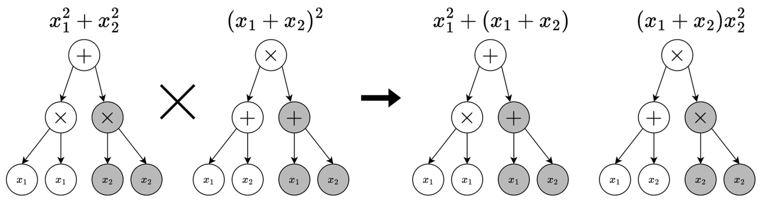
The crossover operator is defined as

$$cross\left(V_p,V_q\right)$$

where $V_p$ and $V_q$ are two parent individuals chosen via selection, and $p_c$ is the predefined crossover probability. With probability $p_c$, a random node is selected in the tree representations of both parents $V_p$ and $V_q$. The corresponding subtrees are swapped, generating two offspring that inherit genetic material from both parents, introducing new variations. If crossover is not performed (with probability ${1-p}_c$), the parent individuals are passed forward unchanged. Figure 1 illustrates the crossover operation, where shaded nodes are selected to be swapped between parents.

The mutation operator is defined as

$$mutate\left(V,p_m\right),$$

where $V$ is an individual (either offspring of crossover or a direct parent copy), and $p_m$ is the mutation probability. With probability $p_m$, a random node in the tree representation of $V$ is replaced with a newly generated subtree constructed using the recursive initialization procedure. If no mutation occurs (with probability ${1-p}_m$), then $V$ is retained in the offspring pool if it results from crossover; however, if $V$ is a direct copy of a parent, it is removed to avoid stagnation and promote population diversity. Figure 2 illustrates the mutation operation, where shaded nodes from the individual were replaced by a randomly generated subtree.

These operations are repeated until the offspring pool reaches the desired size of $\lambda$. After the offspring pool is fully populated, each individual’s fitness from the offspring pool is evaluated using the empirical Lyapunov fitness (4).

Step 4.

Forming a New Generation.

Following the $\left(\mu +\lambda \right)-ES$, we merge the current generation with the offspring pool, forming a combined pool of size $\gamma =\mu +\lambda$.

All individuals in this pool are ranked by fitness, and the top $\mu$ (i.e., those with the lowest fitness values) are selected to form the next generation. This elitist strategy ensures the survival of the best-performing individuals from the previous generation while allowing new variations to improve diversity. This balance enhances convergence and maintains stability in the evolutionary process.

Step 5.

Termination Check.

The algorithm continues to evolve until one of the following stopping criteria is met:

• Maximum Generations Reached: The algorithm runs for a predefined number of generations $n_g$, after which the algorithm terminates.
• Early Stopping: If an individual achieves a predefined target fitness value of 0.
• No Improvement: If the best fitness value remains unchanged for $n_b$ consecutive generations, the algorithm is considered converged, and execution stops.

These termination conditions ensure computational efficiency, preventing unnecessary iterations while striving for optimal solutions.

5. Experiments

In this section, we validate the proposed algorithm by constructing polynomial Lyapunov functions for several nonlinear dynamical systems.

We implemented an application for numerical experiments. The environment parameters of the workstation and environment are as follows:

• Programming language: Python 3.13.
• Libraries:
  • Symbolic computations: PySR 1.4.0 [24].
  • Evolutionary algorithms framework: DEAP 1.4.2 [25].
  • Visualization: Matplotlib 3.10.0 [26].
• Algorithm settings:
  • Initial population size: $G=1000$.
  • Maximum number of generations: $n_g=100$.
  • Number of individuals selected for the next generation: $\mu =500$.
  • Number of offspring: $\lambda =250$.
  • Crossover probability: $p_c=0.2$.
  • Mutation probability: $p_m=0.1.$
  • Number of random test points: $N=5000$.
• Constraints:
  • Domain of interest: $D=\left\{x\in {\mathbb{R}}^n \right| {‖x‖}_2\le 1\}$.
  • Constants $\left\{a_1,\dots ,a_n\right\}\subset \mathbb{Z}$.

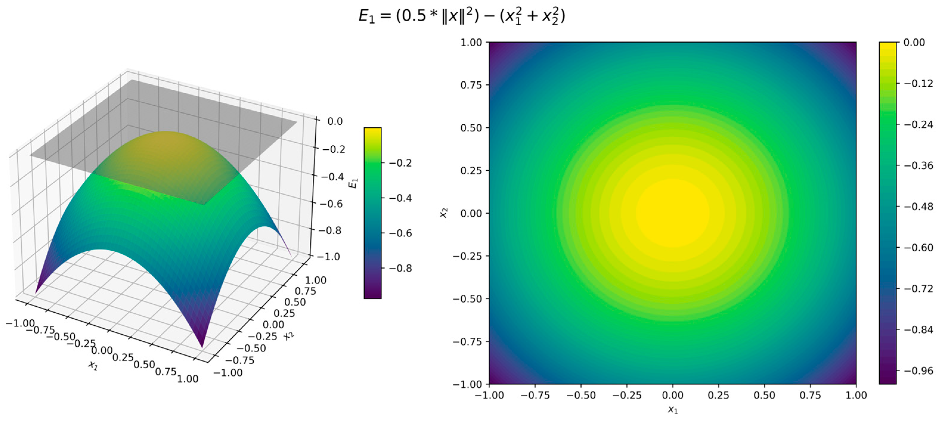
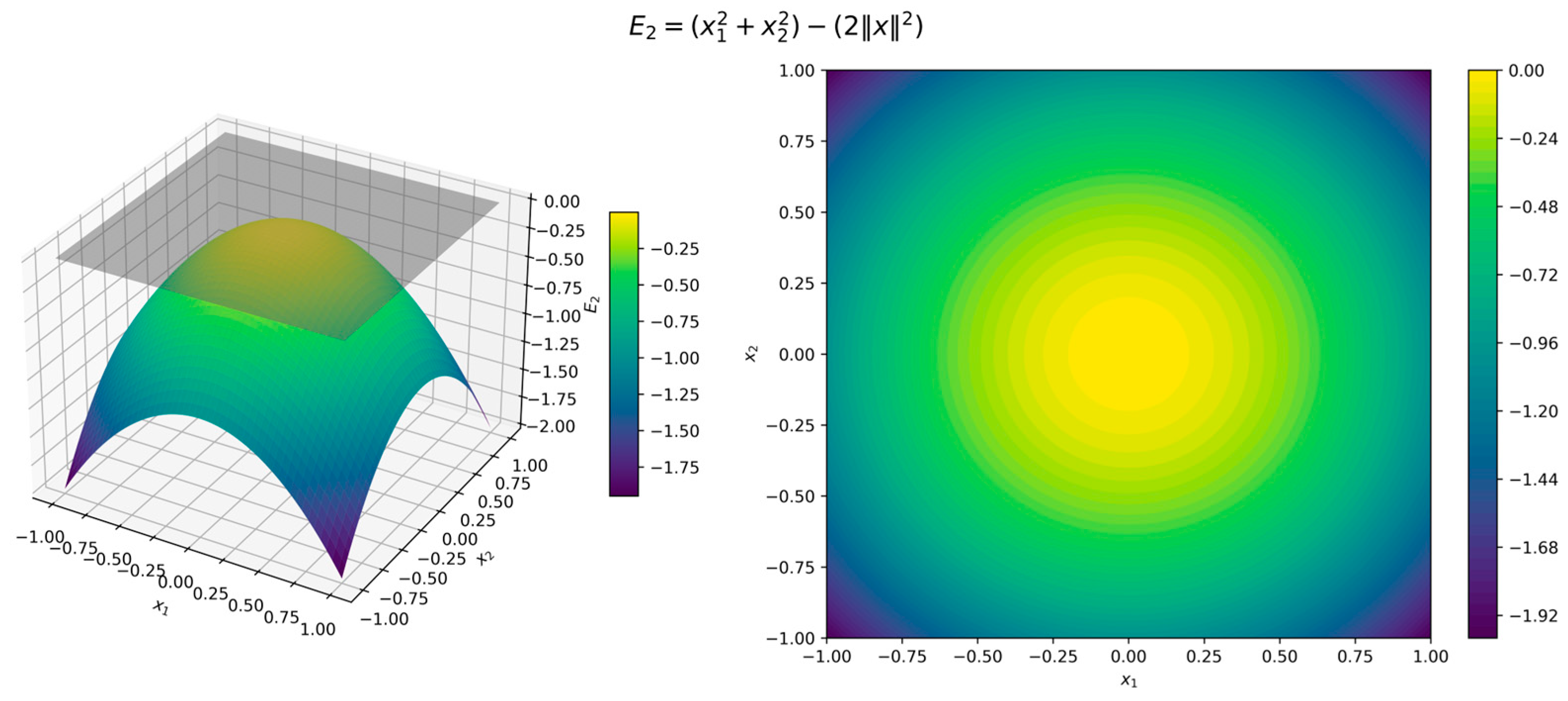
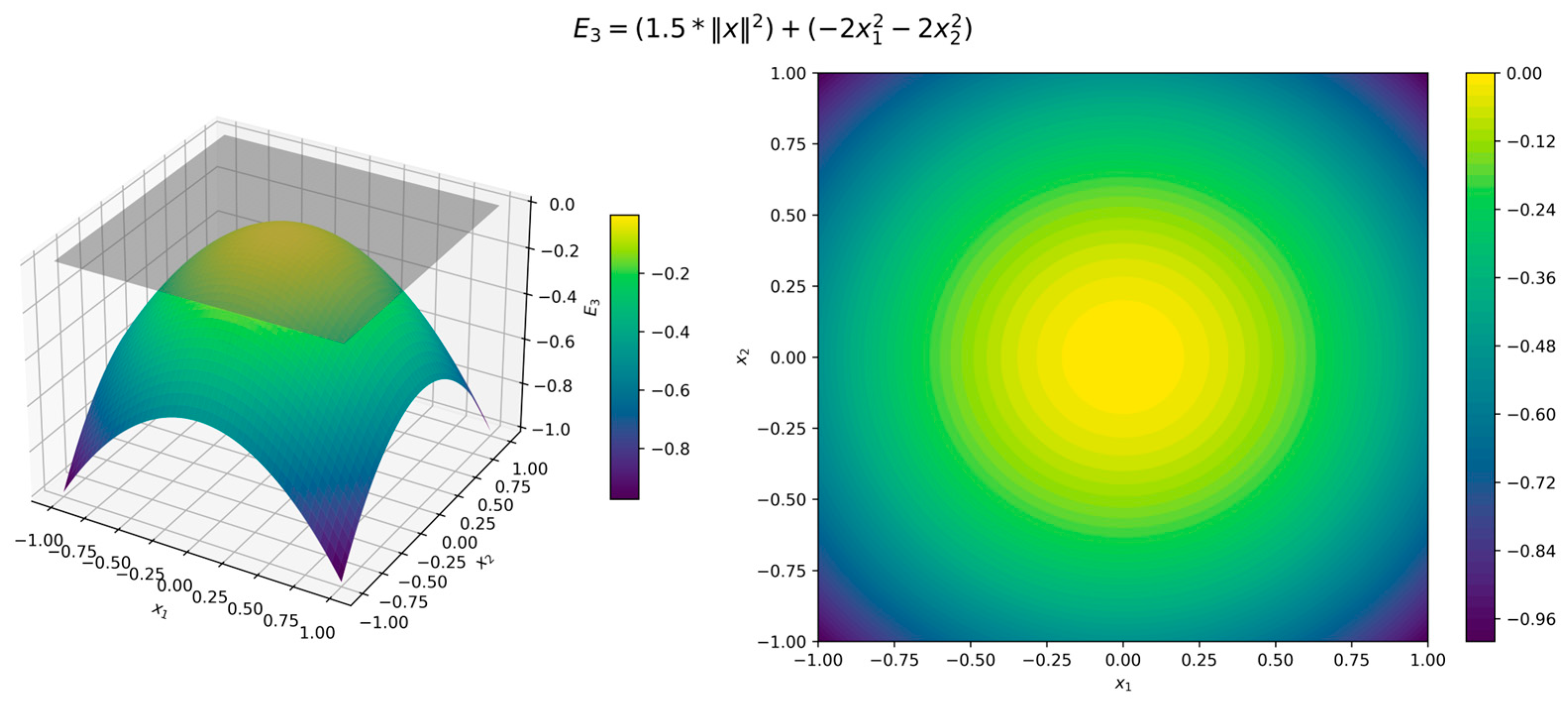
For visualization purposes, we define three error functions:

$$E_1\left(x\right)=k_1{‖x‖}^2-V\left(x\right),$$

(7)

$$E_2\left(x\right)=V\left(x\right)-k_2{‖x‖}^2,$$

(8)

$$E_3\left(x\right)=k_3{‖x‖}^2+\nabla {V\left(x\right)}^{T}f\left(x\right),$$

(9)

which correspond to the lower-bound, upper-bound, and dissipation penalties, respectively. They are each expected to be non-positive on a chosen domain to satisfy (2) and to ensure the exponential stability conditions are met.

Example 1: 

Simple Two-Dimensional Linear System

$$\left\{\begin{array}{c}\dot{x_1}=-x_1,\\ \dot{x_2}=-x_2.\end{array}\right.$$

(10)

This system describes two independent, exponentially stable modes, where each state variable decays exponentially to the origin.

After two iterations, the algorithm identified the following quadratic function, which is commonly used as an initial guess for a Lyapunov function:

$$V\left(x\right)=x_1^2+x_2^2={‖x‖}^2.$$

(11)

It is straightforward to verify that $V$ is a valid Lyapunov function for this system. Its orbital derivative is

$${V\left(x\right)}^{T}f\left(x\right)=-2\left(x_1^2+x_2^2\right)=-2{‖x‖}^2.$$

(12)

Thus, the exponential stability conditions are satisfied for any neighborhood of the origin with the constants $k_1,k_2=1$ and $k_3=2$.

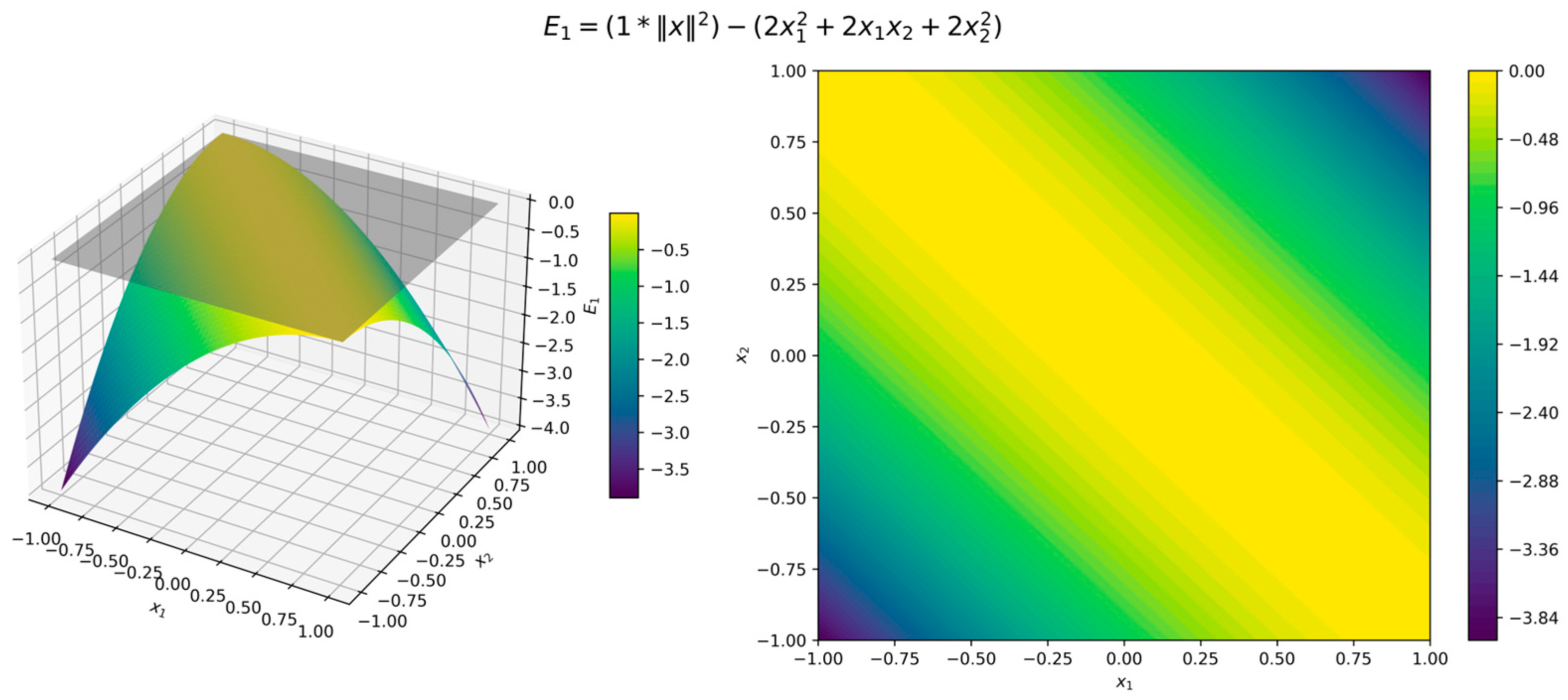
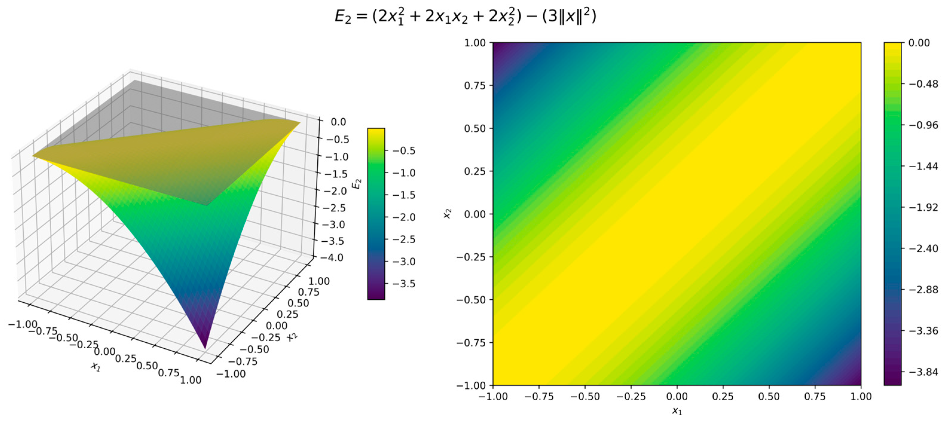
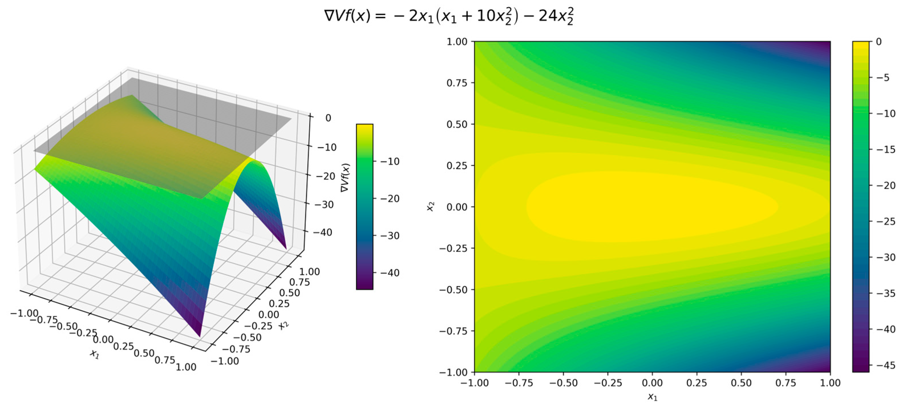
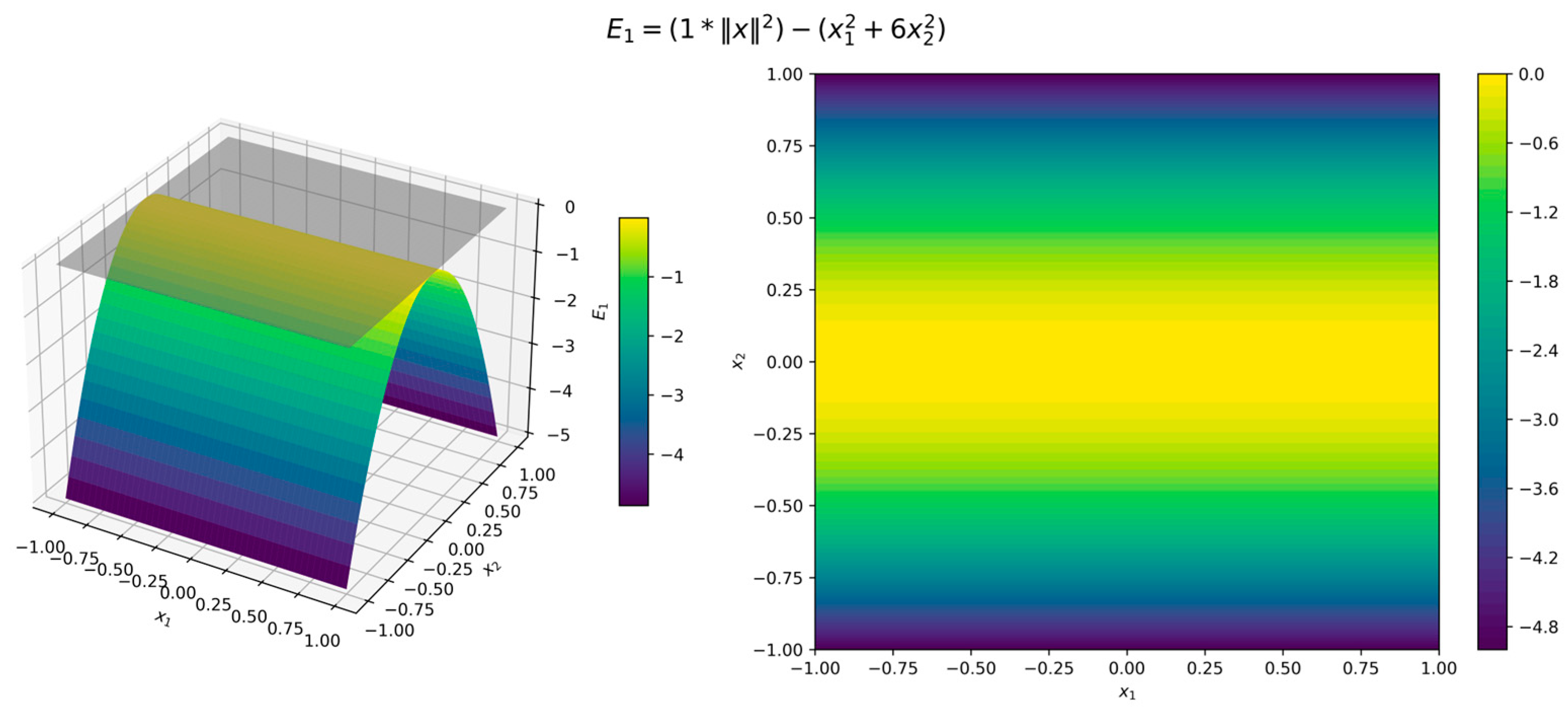
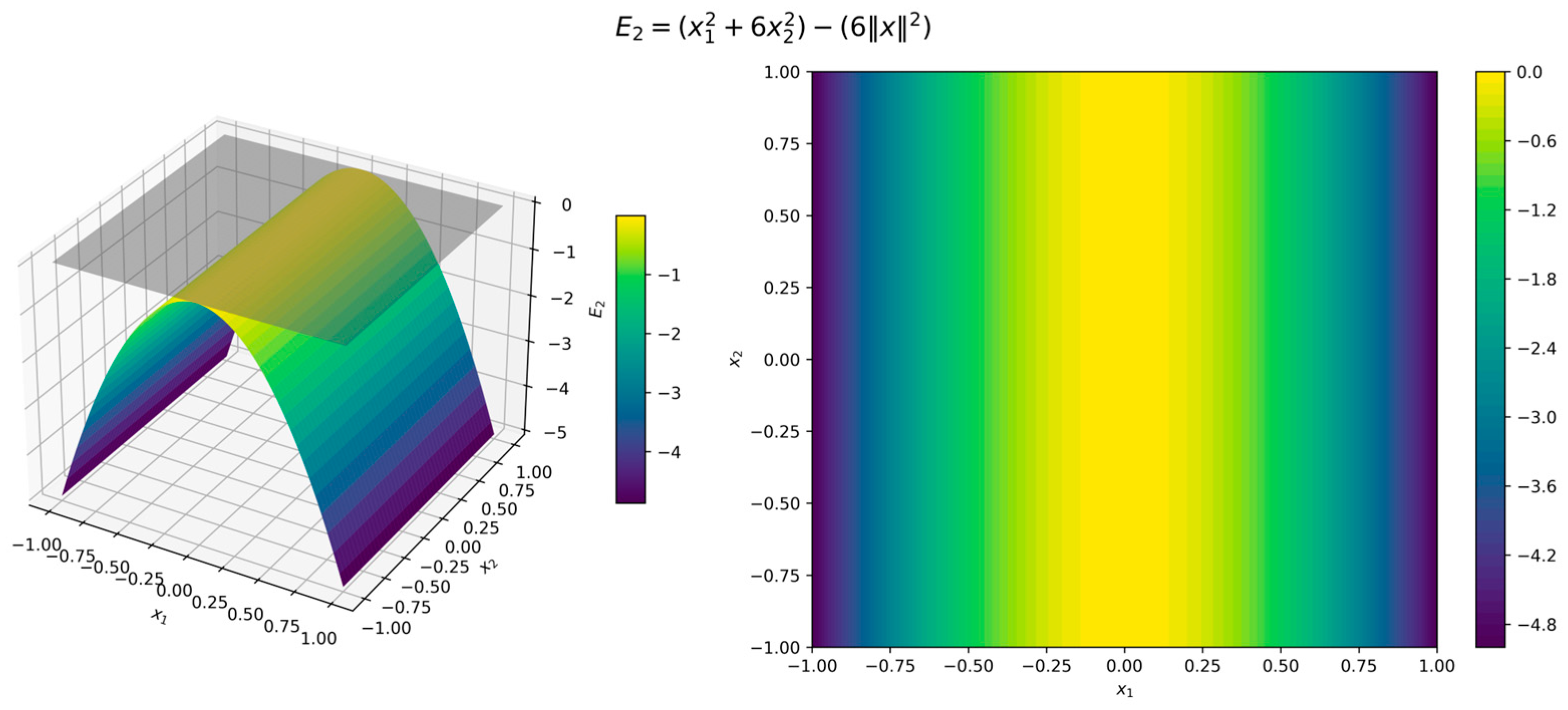
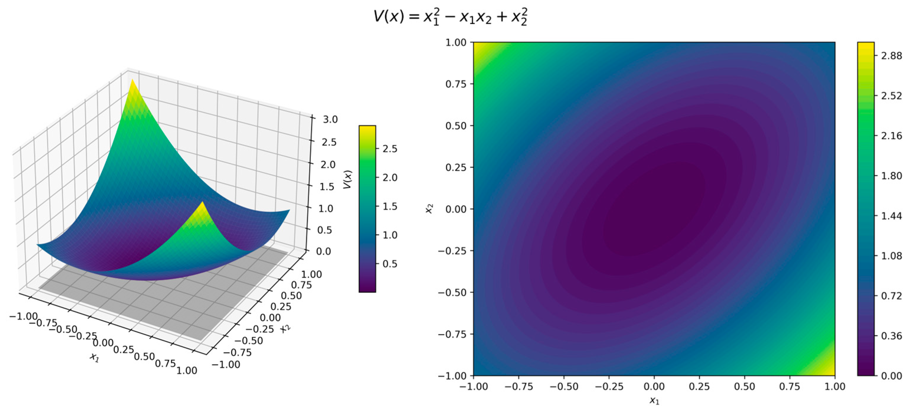
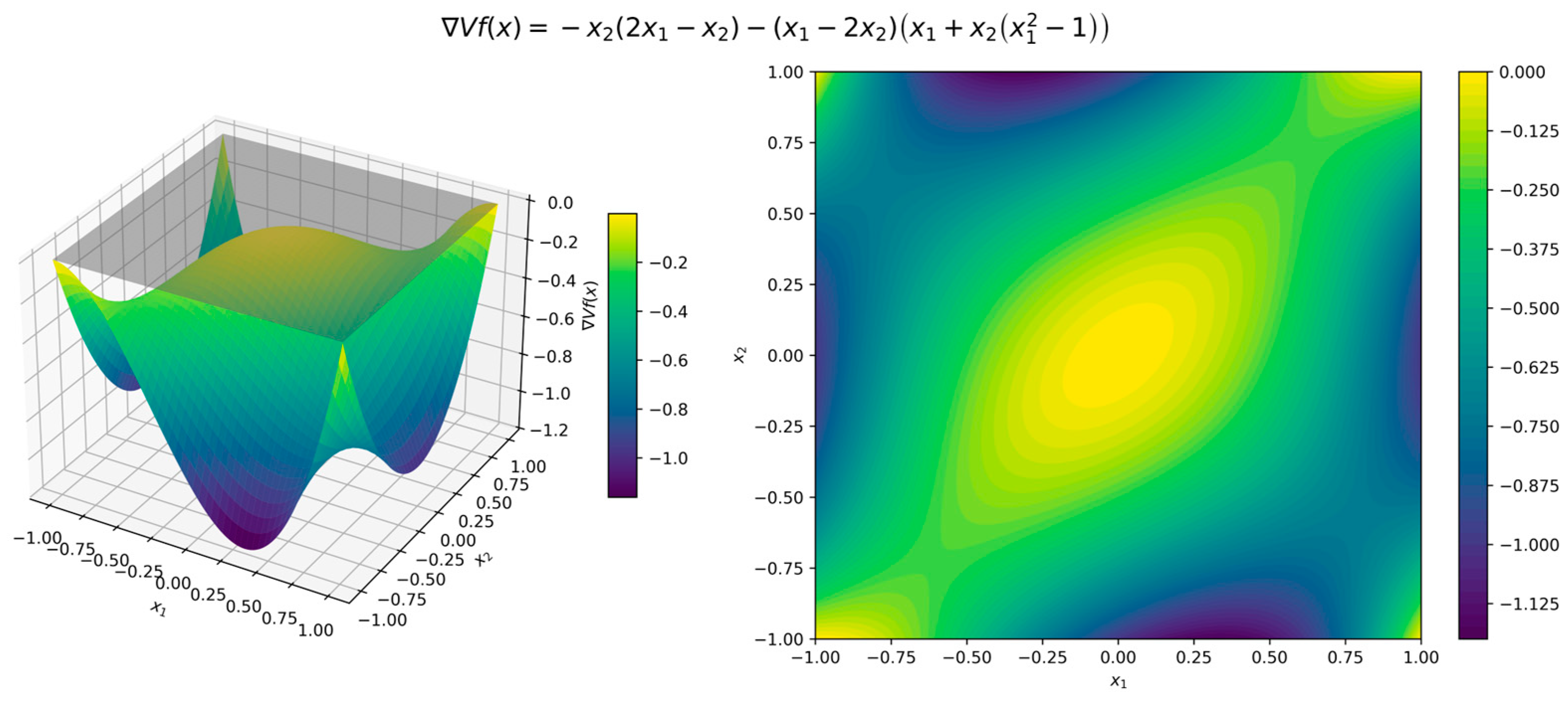
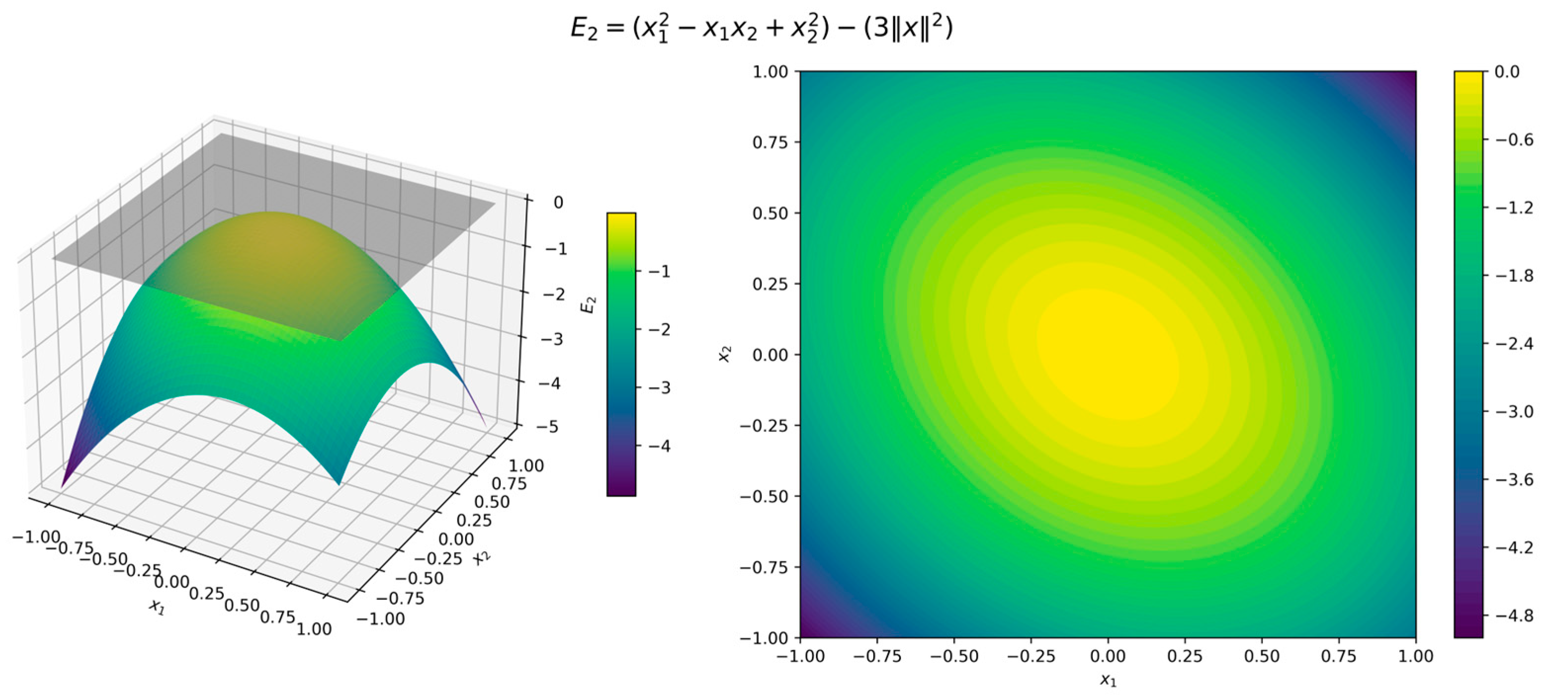
The surface and contour plots of the Lyapunov function (11) in Figure 3 illustrate its quadratic form, where the level sets form concentric circles centered at the origin, while the orbital derivative (12) in Figure 4 confirms strict negativity across all directions. Although the error functions (7)–(9) are 0 when $k_1,k_2=1$ and $k_3=2$, for illustration we used $k_1=0.5$, $k_2=2$, and $k_3=1$. Figure 5, Figure 6 and Figure 7 present surface and contour plots of the errors $E_1, E_2, E_3$ using illustrative parameters.

Example 2: 

The Damped Pendulum

$$\left\{\begin{array}{c}\dot{x_1}=x_2,\hfill \\ \dot{x_2}=-sin\left(x_1\right)-x_2.\end{array}\right.$$

(13)

This is a classic example of a nonlinear dynamical system. This system satisfies the conditions of Theorem 4, where the Hurwitz linearization matrix at the equilibrium point $x^{*}=0$ confirms the exponential stability of the origin.

The algorithm successfully identified the following quadratic Lyapunov function in the ninth generation:

$$V\left(x\right)=2x_1^2+2x_1{x}_2+{2x}_2^2.$$

(14)

The orbital derivative is

$$\nabla {V\left(x\right)}^{T}f\left(x\right)=2x_2\left(2x_1+x_2\right)-2\left(x_1+{2x}_2\right)\left(x_2+sin\left(x_1\right)\right).$$

(15)

The Lyapunov function guarantees the exponential stability of the damped pendulum system (13) within the domain $‖x‖\le 1$ and constants $k_1=1,k_2=3$, and $k_3=1$.

Figure 8 presents the surface and contour plots of the Lyapunov function (14), highlighting its quadratic form, where the level sets form concentric ellipses centered at the origin. The corresponding orbital derivative (15), shown in Figure 9, confirms strict negativity across all directions. Additionally, Figure 10, Figure 11 and Figure 12 present the surface and contour plots of the errors $E_1, E_2, E_3$, visually confirming that the exponential stability conditions of the origin are met.

Example 3: 

A Two-Dimensional Polynomial System

$$\left\{\begin{array}{c}\dot{x_1}={-x}_1-10x_2^2,\\ \dot{x_2}=-2x_2.\hfill \end{array}\right.$$

(16)

This example, presented in [11], examines a two-dimensional system that employs a compositional Lyapunov function. This system meets the criteria of Theorem 4, where the Hurwitz linearization matrix at the equilibrium point $x^{*}=0$ confirms the exponential stability of the origin.

The algorithm successfully identified the Lyapunov function after 16 iterations:

$$V\left(x\right)=x_1^2+6x_2^2.$$

(17)

The orbital derivative is

$$\nabla {V\left(x\right)}^{T}f\left(x\right)=-2x_1\left(x_1+10x_2^2\right)-24x_2^2.$$

(18)

The Lyapunov function (17) ensures that the polynomial system (16) is exponentially stable within the domain $‖x‖\le 1$ and constants $k_1=1,k_2=6$, and $k_3=2$.

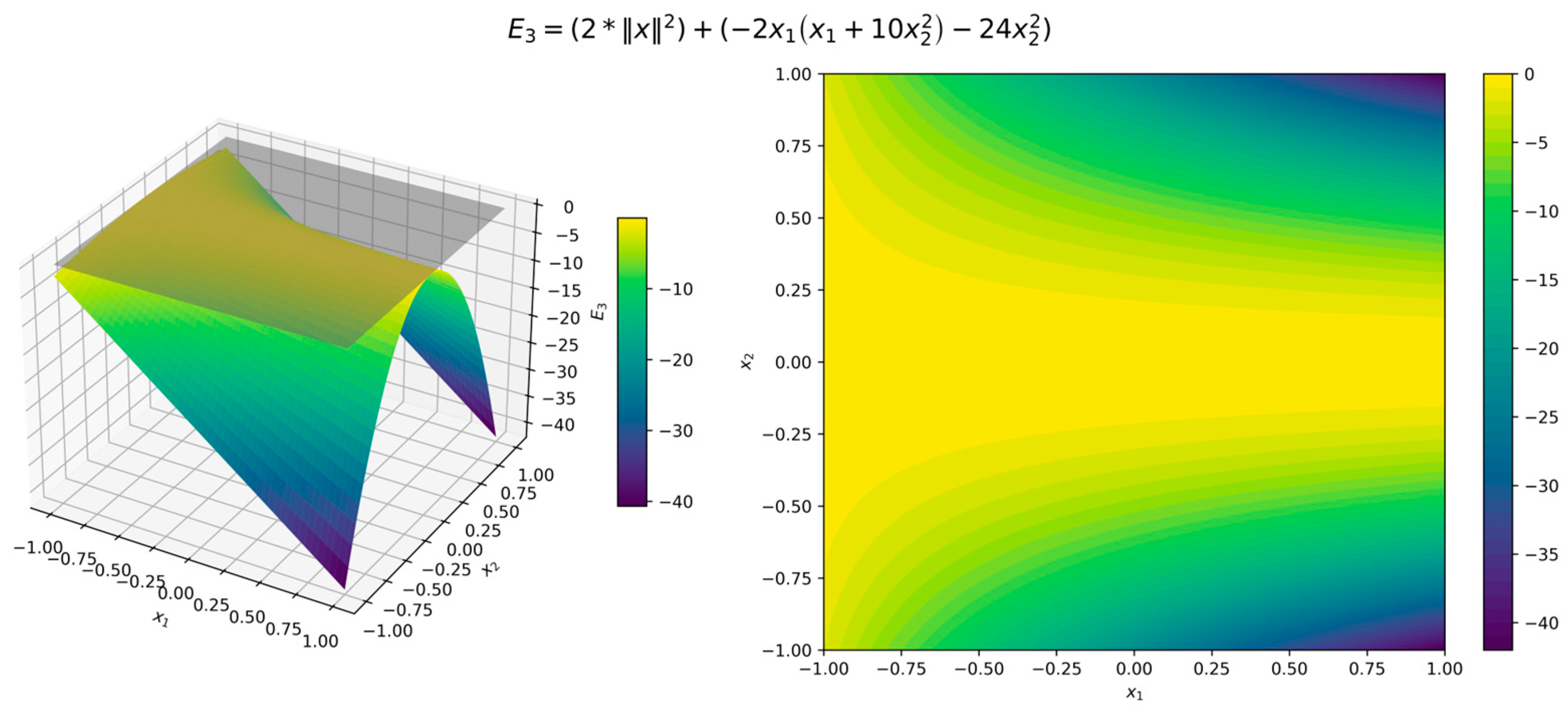
Figure 13 shows the surface and contour plots of function (17), visually confirming its properties. Figure 14 shows that the orbital derivative is negative over the considered domain. Figure 15, Figure 16 and Figure 17 display the surface and contour plots of the error functions $E_1, E_2$, and $E_3$, providing additional insight into the effectiveness of (17) in capturing the stability characteristics of the polynomial system (16).

Example 4: 

The Van der Pol Oscillator

$$\left\{\begin{array}{c}\dot{x_1}={-x}_2,\hfill \\ \dot{x_2}=x_1+x_2\left(x_1^2-1\right).\end{array}\right.$$

(19)

This system provides another classic example of a nonlinear dynamical system—a Van der Pol equation in reverse time, that is, with $t$ replaced by $-t$. It fulfills the conditions outlined in Theorem 4, with the Hurwitz linearization matrix at the equilibrium point $x^{*}=0$, thus verifying the exponential stability of the origin.

The algorithm successfully identified the Lyapunov function in the twelfth generation:

$$V\left(x\right)=x_1^2-x_1{x}_2+x_2^2.$$

(20)

The orbital derivative is

$$\nabla {V\left(x\right)}^{T}f\left(x\right)=-x_2\left(2x_1-x_2\right)-\left(x_1-2x_2\right)\left(x_1+x_2\left(x_1^2-1\right)\right).$$

(21)

The Lyapunov function guarantees the exponential stability of the Van der Pol system (19) within the domain $‖x‖\le 1$ and constants $k_1=0.1,k_2=3$, and $k_3=0.1$.

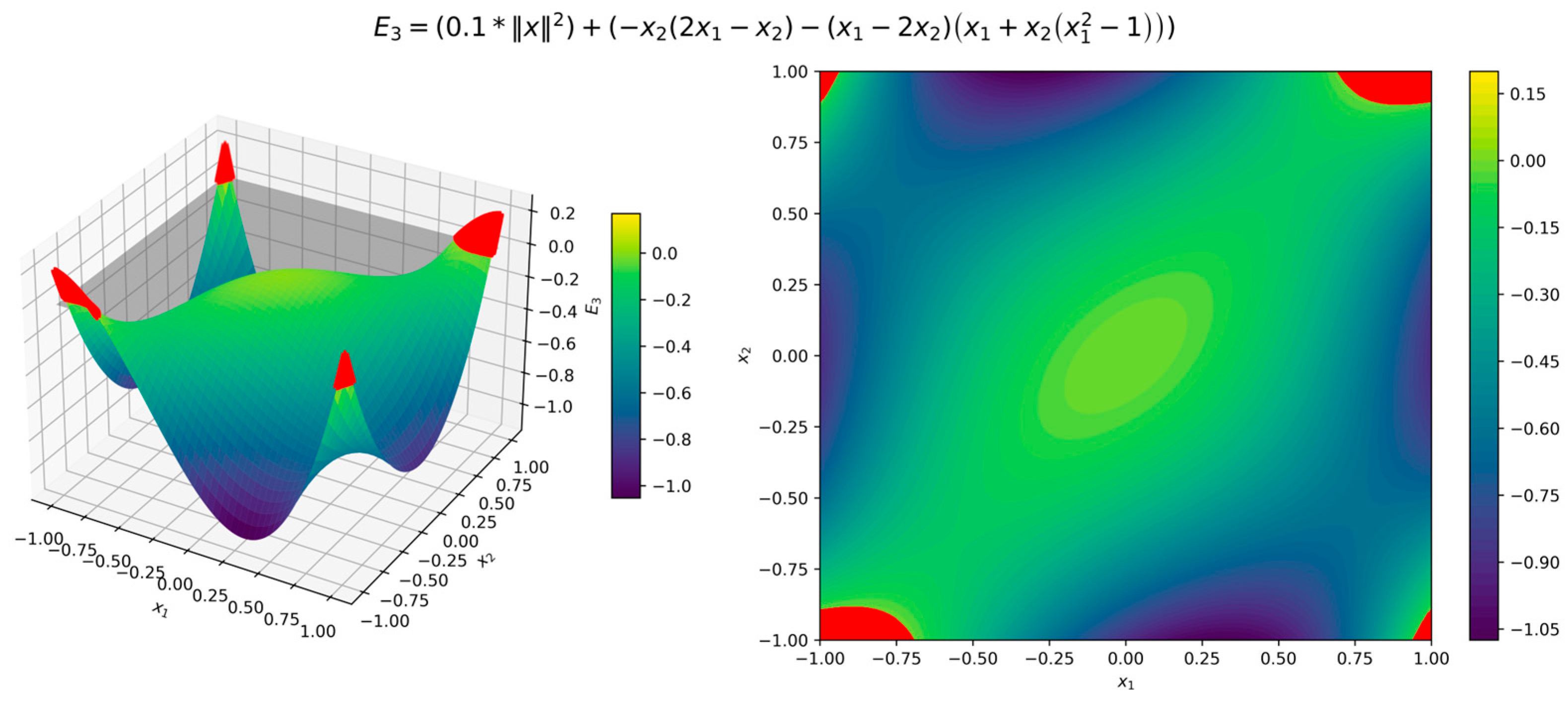
Figure 18 shows the surface and contour plots of function (20), visually confirming its properties. Figure 19 depicts the orbital derivative, revealing the intricate nonlinear dynamics of the system. Figure 20, Figure 21 and Figure 22 display the surface and contour plots of the error functions $E_1, E_2, E_3$, offering further insight into the accuracy with which function (20) represents the stability properties of the Van der Pol system (19). The red region in Figure 22 indicates areas where $E_3>0$, meaning the dissipation conditions are not met. However, this region falls outside the domain $D.$

6. Discussion

Our numerical experiments demonstrate that a GP-based search for polynomial Lyapunov functions reliably verifies stability of nonlinear systems. The fitness metric (4) employed in our GP-based method was specifically designed to enforce both positivity and dissipation conditions, ensuring that every Lyapunov criterion is satisfied. This metric effectively steered the evolutionary process toward valid polynomial solutions in our numerical tests. Additionally, the method’s inherent flexibility allows it to adapt to a variety of problem configurations and complexities. However, further work is needed to optimize the algorithm for higher-dimensional systems.

Future research can build on this work in several promising directions:

• Enlarging the domain of attraction: Refinements are required to systematically expand the region over which the Lyapunov function remains valid. By prioritizing domain extensions in GP, the resulting Lyapunov function could cover a larger portion of the state space, yielding stronger stability guarantees.
• Enhanced constant selection and optimization: This approach can be strengthened further by developing advanced heuristics and adaptive strategies for tuning the numerical constants, including the terminal node constants $\left\{a_1,\dots ,a_n\right\}$ and the Lyapunov fitness coefficients $k_1, k_2$, and $k_3$. These enhancements could mitigate convergence to suboptimal solutions, optimize computational load, and improve the method’s effectiveness in estimating viable solutions.
• Compositional analytical functions for high-dimensional systems: For larger-scale systems, adapting the algorithm to construct compositional (separable or modular) Lyapunov functions is promising. Such an adaptation could mitigate the curse of dimensionality while preserving solution interpretability in complex, real-world applications.

Additionally, our GP-based method can be extended to the control domain by generating control Lyapunov functions to facilitate the design of robust feedback controllers. Future work could also explore theoretical convergence guarantees, performance bounds, and the integration of these evolutionary methods with classical control techniques to develop a unified framework that combines the strengths of both data-driven and analytical approaches in stability analysis.

7. Conclusions

In this paper, we proposed a genetic programming-based method to construct polynomial Lyapunov functions for exponentially stable nonlinear systems. In Theorem 4, we established the existence criterion for these functions, which serves as the primary indicator of the method’s applicability. We also introduced the Lyapunov fitness (3) to quantify deviations from exponential stability conditions.

We validated the method through numerical experiments on several dynamical systems, including a simple linear system (10), a damped pendulum (13), a polynomial system (16), and the Van der Pol oscillator (19). These tests demonstrate that the proposed method effectively constructs Lyapunov functions and can be used as an automated tool for stability analysis.

The future directions outlined highlight the potential to further enhance and extend the proposed approach. This work offers a flexible, automated method for Lyapunov-based stability certification, bridging evolutionary computation with classical control theory.