1. Introduction
At the planning and estimate stages, the utilization of auxiliary information is important to improving the performance of estimators in survey sampling. The median often gives a more accurate picture of the central tendency than the mean when working with highly skewed data distributions, such as those in income, expenditure, taxation, consumption, and production. For datasets with significant skewness, this is especially true because the median provides a more reliable representation of the information in the middle. The development of effective techniques for accurately estimating medians in finite populations has received less attention, despite the massive quantity of research on estimating population parameters, such as means, variances, proportions, and totals. This contrast highlights the importance of more research on improving methods that use auxiliary variables to improve median estimation. More details about auxiliary information can be found in [
1,
2,
3,
4,
5].
In many cases, the median is important for analyzing skewed data or outliers. For reflecting survey responses in the social sciences, income in economics, pollution levels in environmental research, patient outcomes in health, and variations in the real estate market, it increases statistical accuracy. The estimation of the median using auxiliary information in simple random sampling has been significantly enhanced by the fundamental contributions [
6,
7,
8,
9]. Their efforts laid the foundation for subsequent research and enhancement in this area. A number of estimators have been developed for estimating the finite population median using various sampling techniques in subsequent years of the work [
9]. Some novel techniques for improving regression estimators and ratios for the median were proposed by [
10]. To address median estimation, ref. [
11] presented a few techniques utilizing double sampling techniques. The population median was estimated by [
12] using a generalized class of estimators that employs two auxiliary variables in double sampling. By employing the known median of the auxiliary variable, ref. [
13] presented the minimum unbiased estimator. Subsequently, later on, the accuracy of the median estimation was improved by using two auxiliary variables under the two-phase sampling technique as discussed by [
14]. To approximate the population median using simple random and stratified random sampling methods, refs. [
15,
16] developed several improved estimators. Using auxiliary data for various population parameters under different sampling designs, some new estimators were developed by [
17,
18,
19]. In recent years, many researchers have been focusing on introducing new efficient estimators to estimate population median with different sampling methods. For more details about median estimation, we refer the reader to [
20,
21,
22,
23,
24,
25,
26,
27], and references therein.
The precision of estimators typically decreases and may lead to misleading results when extreme values are present. All ratio, product, regression, and exponential estimators used to determine the finite population median significantly rely on traditional auxiliary variable measures, which is a drawback. This dependence can reduce their efficacy, especially in outlier-influenced datasets. An efficient estimator can reduce both bias and mean squared error to provide more accurate results by using the transformation strategy. In this paper, an enhanced class of ratio–product types of estimators is introduced that employs the transformation technique by linearly combining two robust measures, the trimean and decile mean, and five non-conventional measures, the inter-quartile range, mid-range, quartile average, and quartile deviation, on auxiliary variables with a simple random sampling method to estimate the finite population median. This transformation approach improves efficiency and helps estimators manage data variability. The suggested estimators are flexible to skewed distributions and datasets with outliers, in contrast to many other estimators previously in use. Because of their flexibility, they are especially useful in domains such as environmental research, healthcare, and income analysis.
Real-Life Applications
In real-life applications, the improved median-estimation method proposed in this study can provide valuable insights across various fields:
Economic income-distribution analysis: In economics, accurate estimations of median income are crucial for understanding income inequality. The proposed method can offer more reliable median estimates even in the presence of extreme incomes or outliers, providing a clearer understanding of wealth distribution, which is critical for policy making and economic planning.
Climate research: In climate studies, data often contain extreme values due to rare events like heatwaves or storms. By applying the improved median estimation, researchers can obtain a more stable and robust estimate of climate variables (e.g., average temperature or rainfall) without the distortion caused by these extreme outliers. This can improve the reliability of climate models and help in formulating better strategies for climate change adaptation.
Medical studies: In healthcare, particularly when dealing with patient data or clinical trials, outliers can significantly affect the analysis of treatment efficacy or patient outcomes. The proposed method can be instrumental in estimating more accurate median values of health metrics (e.g., blood pressure, cholesterol levels) in populations with heterogeneous health conditions, thus ensuring more robust conclusions and better healthcare decision-making.
Environmental monitoring: For environmental monitoring, where pollutants or rare events (e.g., oil spills, radioactive leaks) can distort data, the improved median estimator can offer a more reliable measure of the central tendency, improving the accuracy of risk assessments and mitigation strategies.
Education and social sciences: The method could be applied in educational assessments or social research, where extreme test scores or outlier responses could otherwise skew the interpretation of central tendencies. By providing more robust median estimates, researchers can better understand the typical performance or behavior in a population, leading to more informed decisions in policy or education strategy development.
The structure of this paper can be outlined as follows:
Section 2 provides a comprehensive explanation of the methods and notations employed in the study, followed by a review of existing estimators in
Section 2 to establish a foundation for comparison.
Section 3 introduces and elaborates on the proposed class of estimators.
Section 4 presents a detailed mathematical comparison of the estimators under consideration. To verify the theoretical findings discussed in this section, a simulation study is conducted in
Section 5. This study involves the construction of five distinct artificial populations utilizing various probability distributions. Furthermore, this section includes numerical examples to illustrate the practical application of the theoretical results. Finally,
Section 6 provides a summary of the key findings and proposes potential paths for future research.
2. Concepts and Existing Estimators
Suppose the auxiliary variable is denoted by X and the study variable by Y for a finite population consisting of N units, denoted as . For each unit i where , the corresponding values of the auxiliary and study variables are and , respectively. Let a random sample of size n be selected from the population of size N with the condition that under simple random sampling without replacement (SRSWOR). The population medians for the study and auxiliary variables are represented as and , and the sample medians as and . The associated probability density functions for the population medians are and . The correlation coefficient between and is denoted by and is defined as where
To determine the mathematical properties of different estimators, the following relative error terms are utilized:
and
such that
for
.
where
denote the population coefficient of variations of the study variable
Y and the auxiliary variable
X, and let
be the finite population-correction factor.
Now, the biases and mean squared errors of the existing estimators used to estimate the finite population mean are investigated. We then compare these results with those of our suggested class of estimators to identify potential improvements.
The population median is generally estimated by the unbiased estimator, defined as:
The variance of
is given by:
Assuming the median of the
X variable is known, ref. [
9] proposed a ratio-type estimator for
, which is defined as:
The following formulas are used to express the bias and MSE of
:
and
The difference estimator for
introduced by [
13] is defined as:
where
d is an unknown constant, and the optimum value of
d is as given below:
The minimum MSE of
is given below:
We present an exponential ratio and product-type estimators in terms of median using the idea provided by [
28]:
and
The biases and MSEs for (
) are as follows:
and
The difference type estimators for estimating median introduced by [
10,
14] are:
The optimum values of the unknown constants
are given below:
and
The minimum biases and mean squared errors of
are given by the following expressions, using the optimal values of
:
and
3. Proposed Family of Estimators
In this section, we discuss a family of ratio–product-type estimators, which employs the transformation technique by linearly combining robust measures such as the trimean and decile mean and five non-conventional measures, the range, inter-quartile range, mid-range, quartile average, and quartile deviation, on auxiliary variables with the simple random sampling method to estimate the finite population median. This transformation approach improves efficiency and helps estimators manage data variability. The proposed estimator is defined below:
where the terms
represent fixed constant values either 1 or 2, while the known population parameters (
) are associated with the auxiliary variable
X. From Equation (
23), a set of new estimators can be derived by varying the population parameters
, including the interquartile range (
), mid-range (
), quartile average (
), quartile deviation (
), tri-mean (
), and decile mean (
), as shown in
Table 1.
The following theorem provides the bias and mean squared error of the family of ratio–product-type estimators
Theorem 1. Consider as a set of ratio–product estimators used to estimate the finite population median in a simple random sampling scheme. The expressions for the bias and mean squared error (MSE) of are provided below:and Proof. To prove this theorem, we recall some concepts:
such that
for
,
and
where
In order to examine the properties of the suggested estimator, we simplify Equation (
23) by expressing it in terms of relative errors, which allows us to calculate the bias and mean squared error (MSE) of
, as follows:
where
and
are defined as:
and
We examine the right-hand side of Equation (
24) using the first-order Taylor series expansion. To simplify, we neglect terms where
, as their contributions are considered negligible in this context. This approach allows us to derive the following key expression:
After simplifying, we obtain:
The bias of
is derived by applying the expectation to both sides of Equation (
25) and replacing the terms (
) with their expected values, which is expressed as:
The MSE of
can be derived by squaring both sides of Equation (
25) and taking the expectation, resulting in the equation shown below:
We can obtain the final results if we substitute the known constant values of
into Equations (
26) and (
27), and after some straightforward simplification, we obtain:
and
□
4. Mathematical Comparison
In this section, we obtain the efficiency conditions by using the mean squared error equations of the proposed family of estimators with the mean squared error equations of existing estimators, such as , , , , , and .
- (i)
The following condition results from comparing the MSE of the new family of estimators proved in (
29) with the variance of the sample median mentioned in (
2):
- (ii)
The following condition results from comparing the MSE of the new family of estimators proved in (
29) with the MSE of the ratio estimator mentioned in (
5):
- (iii)
The following condition results from comparing the MSE of the new family of estimators proved in (
29) with the the MSE of the difference-type estimator mentioned in (
7):
- (iv)
The following condition results from comparing the MSE of the new family of estimators proved in (
29) with the MSE of the exponential ratio-type estimator mentioned in (
12):
- (v)
The following condition results from comparing the MSE of the new family of estimators proved in (
29) with the MSE of the exponential product-type estimator mentioned in (
13):
- (vi)
The following condition results from comparing the MSE of the new family of estimators proved in (
29) with the MSE of difference estimator
mentioned in (
20):
- (vii)
The following condition results from comparing the MSE of the new family of estimators proved in (
29) with the MSE of difference estimator
mentioned in (
21):
- (viii)
The following condition results from comparing the MSE of the new family of estimators proved in (
29) with the MSE of difference estimator
mentioned in (
22):
5. Results and Discussion
To compare the effectiveness of the new family of estimators with all other existing estimators, we generate the five different simulated populations in this part using suitable positively skewed distributions. Additionally, four datasets are used to confirm the performance of the newly suggested estimators.
5.1. Simulation Study
The distribution that is best suited for a median estimate depends on the statistical properties of the data and the distribution itself; the median is particularly helpful and compatible with skewed, outlier-containing, and non-normal data. To obtain the variable X, we chose one of the five distributions provided below:
Population 1: X∼Moderate skew and spread Gamma distribution with
Population 2: X∼Slight skew Log-Normal distribution with
Population 3: X∼Heavy tails Cauchy distribution with
Population 4: X∼Baseline Uniform distribution with
Population 5: X∼High skew Exponential with
For analyzing and showing the robustness of the proposed estimators under different scenarios and their characteristics, these five distributions are most suited. We can use the following equation to find the variable
Y:
where
is the correlation, and
e∼
represents the error term.
We analyzed the MSEs of the proposed estimators and other existing estimators for each distribution and correlation setting using the following techniques proposed by [
29,
30,
31] in the R software (latest v. 4.4.0) to evaluate their robustness and efficiency.
- Step 1:
Using the techniques described above, simulate observations for X and
- Step 2:
Samples of size n were chosen using simple random sampling without replacement (SRSWOR). The sample sizes are and 200.
- Step 3:
To measure the performance of the estimators, compute the required statistics (such as sample mean, median, variance, or covariance) from the sampled data using the procedures outlined above. The optimal values for existing estimators, which consider unknown constants, are also determined.
- Step 4:
For every sample size, MSE values for each estimator discussed in this article are computed.
- Step 5:
After 50,000 iterations of steps 3 and 4, compute the mean squared error values using the formula provided below:
where
t (
) denotes the subscripts of the existing and new family of estimators.
5.2. Real-Life Application
The performance of the suggested family of estimators in comparison with the other estimators is now assessed by analyzing the MSE values of three different datasets. An extensive description of the datasets is given in the following part, along with statistical summaries that emphasize the most significant parameters and characteristics.
Population 1 (Source: [
32]).
Y: Denotes the total number of households; X: Denotes the total area in square miles. Population 2 (Source: [
33]).
Y: Denotes the overall count of educators employed within educational institutions; X: Denotes the overall count of students enrolled in educational institutions in 2012. Population 3 (Source: [
13]).
Y: The overall amount of fish harvested in 1995; X: Denotes the total number of fish harvested by recreational marine fisherman in 1994. Now, proceed with the calculation of mean squared error values for all available estimators. The results of this analysis, which highlight the performance of our proposed family of estimators, can be found in
Table 2.
5.3. Discussion
We performed simulations using suitable distributions with different
values and sample sizes to support the median estimations. The performance of the proposed family of estimators was also evaluated by analyzing three datasets. The mean squared error (MSE) criterion is used to measure the different estimators. From five simulated distributions, the MSE values for the new family and other existing estimators are shown in
Table 3,
Table 4,
Table 5 and
Table 6. The outcomes from the real datasets are shown in
Table 2. We derive the following significant conclusions from these analyses:
The MSE values for all new estimators are less than those of the other existing estimators covered in
Section 2, according to the findings of both simulated and real datasets, which are shown in
Table 2,
Table 3,
Table 4,
Table 5 and
Table 6. This illustrates the better performance of the newly proposed estimators over existing ones.
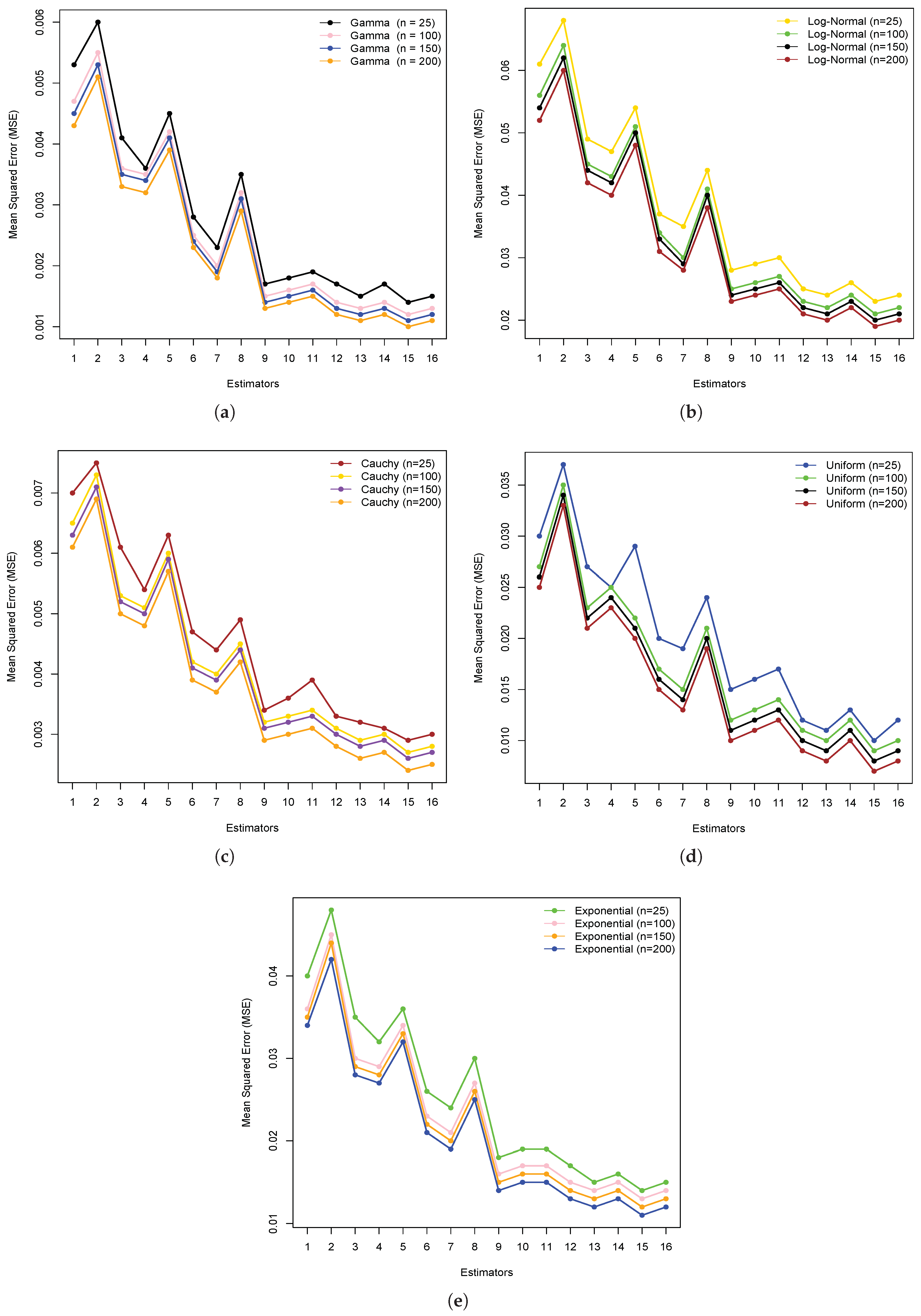
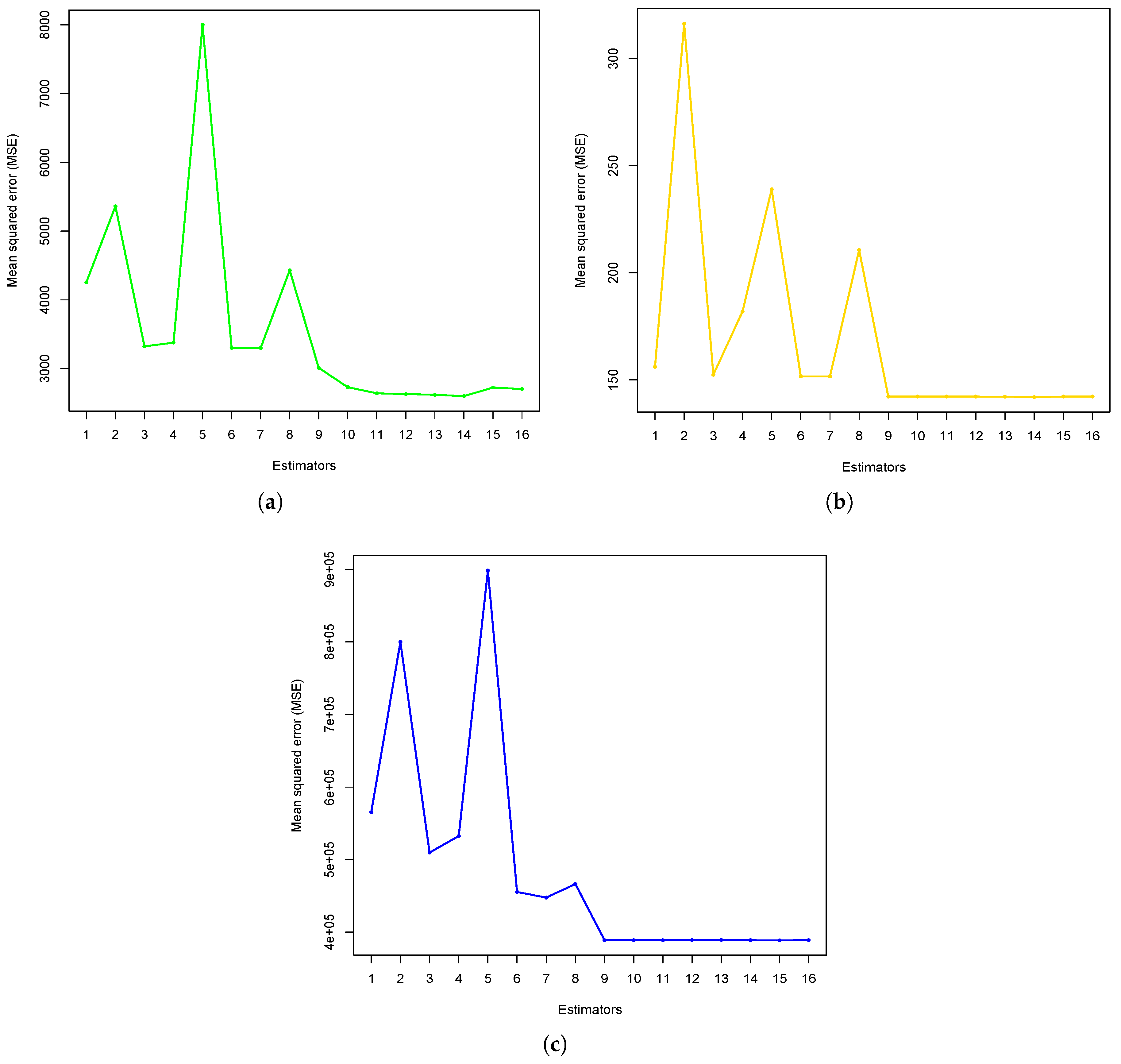
Furthermore, the downward-trending graph lines in
Figure 1 and
Figure 2 for both five simulated distributions and three real datasets prove that all new estimators have MSE values that are consistently lower than those of existing estimators. The inverse relationship between the MSE values for the new estimators and the existing estimators led to the conclusion that the new family of estimators outperforms existing methods.
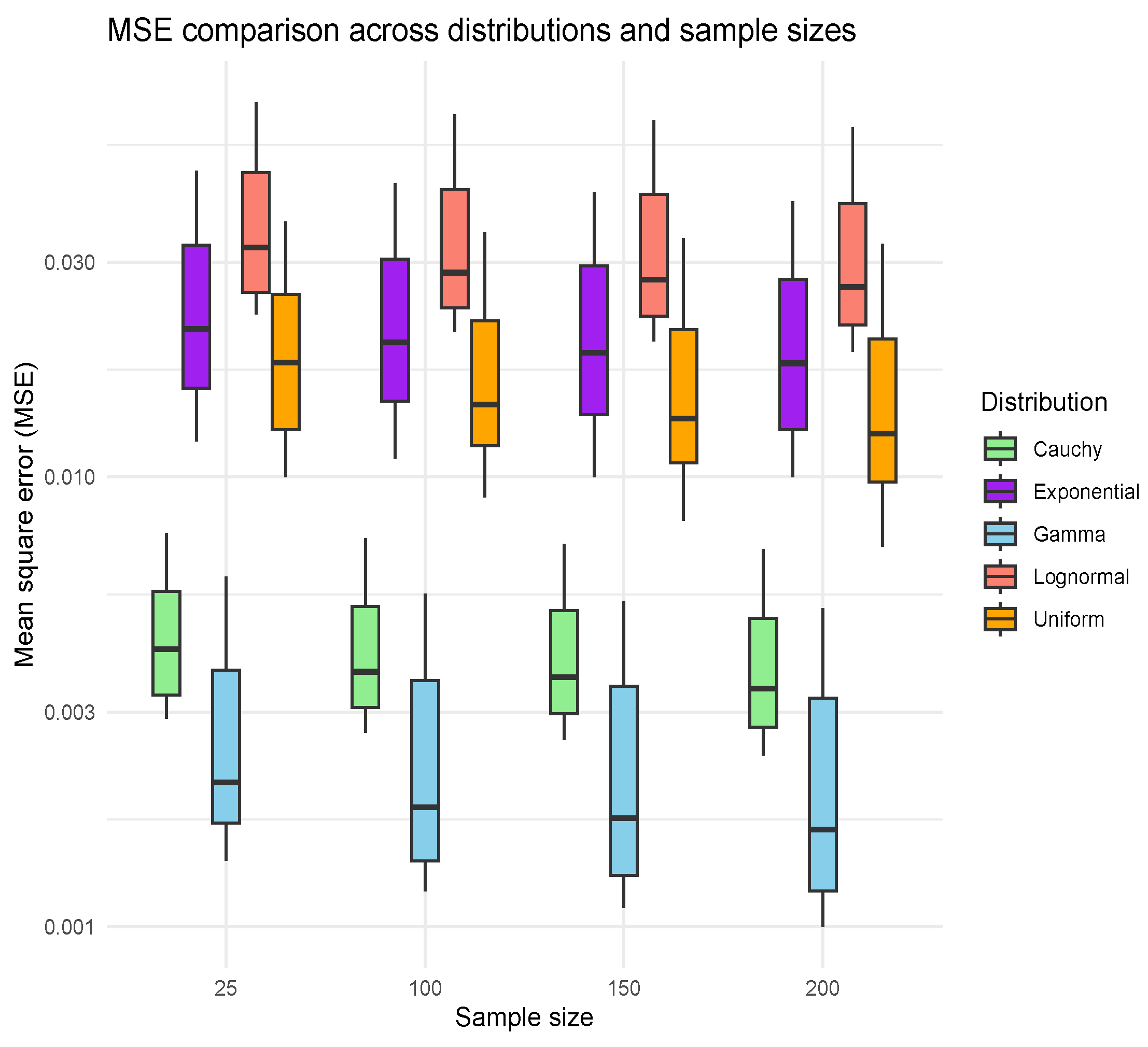
The box plot given in
Figure 3 illustrates the distribution of mean squared error (MSE) values for different sample sizes (25, 100, 150, and 200) across five distributions: Gamma, Lognormal, Cauchy, Uniform, and Exponential. As sample size increases, the MSE values tend to decrease, indicating improved estimation accuracy with larger samples. The plot also highlights variability in MSE across the different distributions, with some showing wider spreads and others demonstrating more consistent performance.
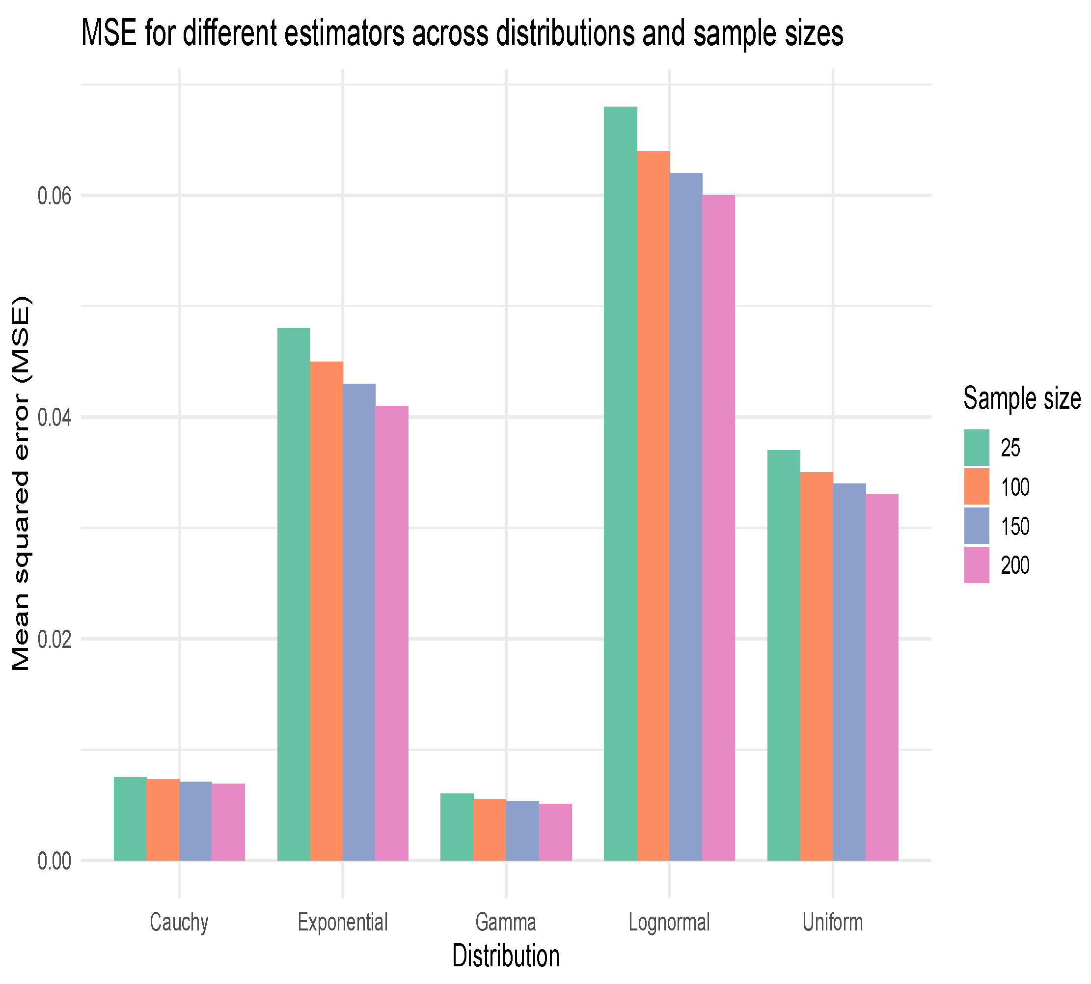
The bar chart displayed in
Figure 4 shows MSE values for different estimators across five distributions and four sample sizes. MSE generally decreases with larger sample sizes, indicating better estimator performance. Distributions like Lognormal and Exponential show higher MSEs, suggesting more estimation difficulty compared to Gamma and Uniform.
6. Conclusions
In this work, we used robust measurements of an auxiliary variable to obtain a new family of estimators to determine the finite population median under simple random sampling. The first degree of approximation provided a valuable framework for obtaining the biases and mean squared errors associated with both existing estimators and several newly developed ones. This approach enhances our understanding of their performance and potential areas for improvement. We conducted simulation analysis through five distributions with all possible different conditions and three real-life datasets to check the potential performance of new estimators with existing estimators by applying the mean squared error criterion. The simulation and numerical real-life dataset results are given in
Table 2,
Table 3,
Table 4,
Table 5 and
Table 6, which show that the new family of estimators performs well and can obtain the optimum estimators as compared to other existing estimators. We noticed that all the new estimators have higher efficiency than other estimators.
The improved median estimation method has broad practical relevance. In economics, it enhances the accuracy of income-distribution analysis by reducing the impact of outliers. In climate research and environmental monitoring, it provides stable estimates despite extreme events, aiding in model reliability and risk assessment. Medical studies benefit from more robust estimates of patient health indicators, leading to sounder conclusions. In education and social sciences, it helps interpret central tendencies accurately, even in the presence of skewed data, thereby supporting better policy and decision-making.
Furthermore, our analysis focused on the properties of the new improved estimators within the context of a simple random sampling technique. It is worth exploring the potential of developing new estimators based on these findings, with the goal of achieving even lower MSE values under systemmatic sampling and stratified random sampling. This topic offers an interesting direction for further investigation.
Author Contributions
Conceptualization, F.A.A. and A.S.A.; methodology, F.A.A. and A.S.A.; software, F.A.A. and A.S.A.; validation, F.A.A. and A.S.A.; formal analysis, F.A.A. and A.S.A.; investigation, F.A.A. and A.S.A.; resources, A.S.A.; data curation, F.A.A. and A.S.A.; writing-original draft preparation, F.A.A. and A.S.A.; writing-review and editing, F.A.A. and A.S.A.; visualization, A.S.A.; supervision, F.A.A.; project administration, A.S.A.; funding acquisition, F.A.A. All authors have read and agreed to the published version of the manuscript.
Funding
Princess Nourah bint Abdulrahman University Researchers Supporting Project number (PNURSP2025R515), Princess Nourah bint Abdulrahman University, Riyadh, Saudi Arabia.
Data Availability Statement
The real data are secondary, and their sources are given in the datasection, while the simulated data have been generated using R software (latest v. 4.4.0).
Conflicts of Interest
The authors declare no conflict of interest.
References
- Zaman, T.; Bulut, H. An efficient family of robust-type estimators for the population variance in simple and stratified random sampling. Commun. Stat.-Theory Methods 2023, 52, 2610–2624. [Google Scholar] [CrossRef]
- Zaman, T.; Bulut, H. A simulation study: Robust ratio double sampling estimator of finite population mean in the presence of outliers. Sci. Iran. 2021, 31, 1330–1341. [Google Scholar] [CrossRef]
- Alghamdi, A.S.; Alrweili, H. New class of estimators for finite population mean under stratified double phase sampling with simulation and real-life application. Mathematics 2025, 13, 329. [Google Scholar] [CrossRef]
- Daraz, U.; Shabbir, J.; Khan, H. Estimation of finite population mean by using minimum and maximum values in stratified random sampling. J. Mod. Appl. Stat. Methods 2018, 17, 20. [Google Scholar] [CrossRef]
- Alomair, M.A.; Daraz, U. Dual transformation of auxiliary variables by using outliers in stratified random sampling. Mathematics 2024, 12, 2829. [Google Scholar] [CrossRef]
- Gross, S. Median estimation in sample surveys. In Proceedings of the Section on Survey Research Methods, Houston, TX, USA, 11–14 August 1980; American Statistical Association Ithaca: Alexandria, VA, USA, 1980. [Google Scholar]
- Sedransk, J.; Meyer, J. Confidence intervals for the quantiles of a finite population: Simple random and stratified simple random sampling. J. R. Stat. Soc. Ser. (Methodol.) 1978, 40, 239–252. [Google Scholar] [CrossRef]
- Philip, S.; Sedransk, J. Lower bounds for confidence coefficients for confidence intervals for finite population quantiles. Commun. Stat.-Theory Methods 1983, 12, 1329–1344. [Google Scholar] [CrossRef]
- Kuk, Y.C.A.; Mak, T.K. Median estimation in the presence of auxiliary information. J. R. Stat. Soc. Ser. B 1989, 51, 261–269. [Google Scholar] [CrossRef]
- Rao, T.J. On certail methods of improving ration and regression estimators. Commun. Stat.-Theory Methods 1991, 20, 3325–3340. [Google Scholar] [CrossRef]
- Singh, S.; Joarder, A.H.; Tracy, D.S. Median estimation using double sampling. Aust. N. Z. J. Stat. 2001, 43, 33–46. [Google Scholar] [CrossRef]
- Khoshnevisan, M.; Singh, H.P.; Singh, S.; Smarandache, F. A General Class of Estimators of Population Median Using Two Auxiliary Variables in Double Sampling; Virginia Polytechnic Institute and State University: Blacksburg, VA, USA, 2002. [Google Scholar]
- Singh, S. Advanced Sampling Theory with Applications: How Michael Selected Amy; Springer Science & Business Media: Berlin/Heidelberg, Germany, 2003; Volume 2. [Google Scholar]
- Gupta, S.; Shabbir, J.; Ahmad, S. Estimation of median in two-phase sampling using two auxiliary variables. Commun. Stat.-Theory Methods 2008, 37, 1815–1822. [Google Scholar] [CrossRef]
- Aladag, S.; Cingi, H. Improvement in estimating the population median in simple random sampling and stratified random sampling using auxiliary information. Commun. Stat.-Theory Methods 2015, 44, 1013–1032. [Google Scholar] [CrossRef]
- Solanki, R.S.; Singh, H.P. Some classes of estimators for median estimation in survey sampling. Commun. Stat.-Theory Methods 2015, 44, 1450–1465. [Google Scholar] [CrossRef]
- Daraz, U.; Wu, J.; Albalawi, O. Double exponential ratio estimator of a finite population variance under extreme values in simple random sampling. Mathematics 2024, 12, 1737. [Google Scholar] [CrossRef]
- Daraz, U.; Wu, J.; Alomair, M.A.; Aldoghan, L.A. New classes of difference cum-ratio-type exponential estimators for a finite population variance in stratified random sampling. Heliyon 2024, 10, e33402. [Google Scholar] [CrossRef]
- Daraz, U.; Alomair, M.A.; Albalawi, O. Variance estimation under some transformation for both symmetric and asymmetric data. Symmetry 2024, 16, 957. [Google Scholar] [CrossRef]
- Shabbir, J.; Gupta, S. A generalized class of difference type estimators for population median in survey sampling. Hacet. J. Math. Stat. 2017, 46, 1015–1028. [Google Scholar] [CrossRef]
- Irfan, M.; Maria, J.; Shongwe, S.C.; Zohaib, M.; Bhatti, S.H. Estimation of population median under robust measures of an auxiliary variable. Math. Probl. Eng. 2021, 2021, 4839077. [Google Scholar] [CrossRef]
- Shabbir, J.; Gupta, S.; Narjis, G. On improved class of difference type estimators for population median in survey sampling. Commun. Stat.-Theory Methods 2022, 51, 3334–3354. [Google Scholar] [CrossRef]
- Subzar, M.; Lone, S.A.; Ekpenyong, E.J.; Salam, A.; Aslam, M.; Raja, T.A.; Almutlak, S.A. Efficient class of ratio cum median estimators for estimating the population median. PLoS ONE 2025, 18, e0274690. [Google Scholar] [CrossRef]
- Iseh, M.J. Model formulation on efficiency for median estimation under a fixed cost in survey sampling. Model Assist. Stat. Appl. 2023, 18, 373–385. [Google Scholar] [CrossRef]
- Hussain, M.A.; Javed, M.; Zohaib, M.; Shongwe, S.C.; Awais, M.; Zaagan, A.A.; Irfan, M. Estimation of population median using bivariate auxiliary information in simple random sampling. Heliyon 2024, 10, e28891. [Google Scholar] [CrossRef]
- Bhushan, S.; Kumar, A.; Lone, S.A.; Anwar, S.; Gunaime, N.M. An efficient class of estimators in stratified random sampling with an application to real data. Axioms 2023, 12, 576. [Google Scholar] [CrossRef]
- Stigler, S.M. Linear functions of order statistics. Ann. Math. Stat. 1969, 40, 770–788. [Google Scholar] [CrossRef]
- Singh, H.P.; Vishwakarma, G.K. Modified exponential ratio and product estimators for finite population mean in double sampling. Austrian J. Stat. 2007, 36, 217–225. [Google Scholar] [CrossRef]
- Daraz, U.; Khan, M. Estimation of variance of the difference-cum-ratio-type exponential estimator in simple random sampling. Res. Math. Stat. 2021, 8, 1899402. [Google Scholar] [CrossRef]
- Daraz, U.; Wu, J.; Agustiana, D.; Emam, W. Finite population variance estimation using Monte Carlo simulation and real life application. Symmetry 2025, 17, 84. [Google Scholar] [CrossRef]
- Daraz, U.; Agustiana, D.; Wu, J.; Emam, W. Twofold auxiliary information under two-phase sampling: An improved family of double-transformed variance estimators. Axioms 2025, 14, 64. [Google Scholar] [CrossRef]
- Murthy, M.N. Sampling Theory and Methods; Statistical Publishing Society: Calcutta, India, 1967. [Google Scholar]
- Koyuncu, K.; Kadilar, C. Family of estimators of population mean using two auxiliary variables in stratified random sampling. Commun. Stat.-Theory Methods 2009, 38, 2398–2417. [Google Scholar] [CrossRef]
| Disclaimer/Publisher’s Note: The statements, opinions and data contained in all publications are solely those of the individual author(s) and contributor(s) and not of MDPI and/or the editor(s). MDPI and/or the editor(s) disclaim responsibility for any injury to people or property resulting from any ideas, methods, instructions or products referred to in the content. |
© 2025 by the authors. Licensee MDPI, Basel, Switzerland. This article is an open access article distributed under the terms and conditions of the Creative Commons Attribution (CC BY) license (https://creativecommons.org/licenses/by/4.0/).


