On a Sum of Two Akash Distributions: Inference and Applications

Abstract

We propose a new distribution which is the sum of two independent Akash (AK) random variables with the same parameter. We refer to this distribution as the AKS distribution. We study the density and some of its properties. We derive the method of moments (MM) and the maximum likelihood (ML) estimator, along with the Fisher information. The performance of the ML estimator is evaluated through a simulation study. In addition, we present two real data applications, demonstrating in these cases the superiority of the AKS distribution compared to two other distributions.

1. Introduction

In recent times, new parametric statistical distributions have been developed and applied to model data in various areas of scientific knowledge. Among these, exponential distribution is one of the most widely used due to its simplicity in terms of properties and parameter estimation. However, alternative distributions to the exponential distribution have been proposed, such as the Lindley distribution (see Lindley [1]), which is particularly useful for modeling lifetime.

A random variable X is said to follow a Lindley (L) distribution, denoted by X∼$L\left(\theta \right)$, if its probability density function (pdf) is given by

$$f_X(x;\theta )={\displaystyle \frac{{\theta }^2}{\theta +1}}(1+x)exp(-\theta x),x>0,$$

(1)

where $\theta >0$ is a shape parameter. The Lindley distribution is derived from a mixture of two components: an exponential distribution with a scale parameter $\theta$ and a gamma distribution with a shape parameter 2 and a scale parameter $\theta$. The mixing ratios for these components are ${\displaystyle \frac{\theta }{1+\theta }}$ and ${\displaystyle \frac{1}{1+\theta }}$, respectively.

The cumulative distribution function (cdf) corresponding to (1) is

$$F_X(x;\theta )=1-\left[1+{\displaystyle \frac{\theta x}{\theta +1}}\right]exp(-\theta x),x>0.$$

(2)

The L distribution has been used in various settings such as engineering, demography, reliability, and medicine, among others. Some researchers who have carried out these studies are Hussain [2], Ghitany et al. [3], Zakerzadeh and Dolati [4], Gómez-Déniz and Calderin-Ojeda [5], Krishna and Kumar [6], Bakouch et al. [7], Shanker et al. [8], Ghitany et al. [9], Al-Mutairi et al. [10], Oluyede and Yang [11], Shanker et al. [12], and Abouammoh et al. [13], among others. Similar to the L distribution, the AK distribution is generated based on a mixture of two components: an exponential distribution with a scale parameter $\theta$ and a gamma distribution with a shape parameter 3 and a scale parameter $\theta$. The mixing ratios for these components are ${\displaystyle \frac{{\theta }^2}{2+{\theta }^2}}$ and ${\displaystyle \frac{2}{2+{\theta }^2}}$, respectively. Shanker [14] introduced the AK distribution and applied it to real lifetime data sets from medical science and engineering. Thus, we say that a random variable Y has an AKdistribution with shape parameter $\theta$ if its pdf is given by

$$f_Y(y;\theta )={\displaystyle \frac{{\theta }^3}{({\theta }^2+2)}}(1+y^2)exp(-\theta y),y>0,$$

(3)

where $\theta >0$ is a shape parameter, and it is denoted by Y∼$AK\left(\theta \right)$.

In Figure 1, we show the pdf of the AK distribution for several values of $\theta$. We refer the reader to Figure 1 in Shanker [14] for other plots of the AK distribution.

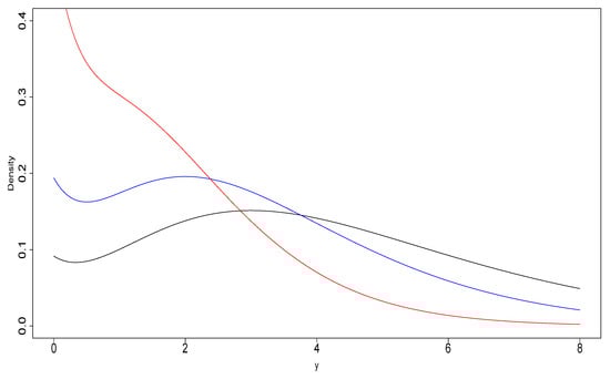
Figure 1. Examples of the AK$\left(0.6\right)$ (black color), AK$\left(0.8\right)$ (blue color), and AK$\left(1.2\right)$ (red color).

Some Properties of This Pdf Are

(a)

The cdf of Y is

$$F_Y(y;\theta )=1-\left[1+{\displaystyle \frac{\theta y(\theta y+2)}{{\theta }^2+2}}\right]exp(-\theta y),y>0.$$

(4)

(b)

For $r=1,2,3,\dots ,$ the r-th moment of Y is

$${\displaystyle \mathbb{E}\left(Y^r\right)=\frac{r!\left[{\theta }^2+(r+1)(r+2)\right]}{{\theta }^r({\theta }^2+2)}.}$$

(5)

(c)

The moment generating function ($M_Y\left(t\right)$) is given by

$$M_Y\left(t\right)=\mathbb{E}\left(exp\left(tY\right)\right)={\displaystyle \frac{{\theta }^3}{{\theta }^2+2}}\left[{\displaystyle \frac{{(\theta -t)}^2+2}{{(\theta -t)}^3}}\right],t<\theta$$

(6)

Extensions AK distribution are given by Shanker and Shukla [15,16] and Gómez et al. [17], among others. In particular, we note the contribution of Yaghoubi [18], who explores the distribution of the sum of n independent and identically distributed Akash random variables and several other distributions primarily used in reliability and lifetime data modeling and derives its moments.

In this article, we consider the special case of two independent AK random variables with the same parameter and study their convolution. We give an alternative derivation of the distribution, discuss several interesting properties, and develop inferential procedures. Applications show that it can be an alternative to the AK and L distributions.

This paper develops as follows: In Section 2, we furnish the AKS distribution and its properties. In Section 3, we perform inference by the methods of moments and maximum likelihood, the Fisher information is obtained, and a simulation study is also carried out. In Section 4, applications are made with two real data sets and compared with the AK and L distributions. In Section 5, we provide some conclusions.

2. The AKS Distribution

In this section, we introduce the density function properties of the AKS distribution.

2.1. Density Function

Definition 1. 

We say that a random variable Z has an AKS distribution with shape parameter θ, Z∼$AKS\left(\theta \right)$, if it has the following pdf:

$$f_Z(z;\theta )={\displaystyle \frac{{\theta }^{6}z}{30{({\theta }^2+2)}^2}}(30+20z^2+z^4)exp(-\theta z),z>0,$$

(7)

where $\theta >0$.

In Figure 2, we show the pdf of the AKS distribution for several values of $\theta$.

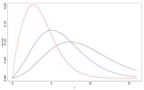
Figure 2. Examples of the AKS$\left(0.6\right)$ (black color), AKS$\left(0.8\right)$ (blue color), and AKS$\left(1.2\right)$ (red color).

2.2. Properties

The following proposition shows that the pdf of the AKS distribution can be obtained from a convolution of two AK distributions:

Proposition 1. 

Let $X_1$∼$AK\left(\theta \right)$, $X_2$∼$AK\left(\theta \right)$ be two independent random variables and define $Z=X_1+X_2$; then, X∼$AKS\left(\theta \right)$.

Proof. 

Since $X_1$ and $X_2$ are independent, the pdf of Z may be obtained from the following convolution product for $x>0$:

$${\displaystyle f_Z(z;\theta )={\int }_0^z{f}_{X_1}(z-t;\theta )f_{X_2}(t;\theta )dt=\frac{{\theta }^{6}exp(-\theta z)}{{({\theta }^2+2)}^2}{\int }_0^z(1+z^2-2zt+t^2)(1+t^2)dt.}$$

By calculating the right-side integral, the result follows.    □

The following proposition shows the cdf of the AKS distribution:

Proposition 2. 

Let Z∼$AKS\left(\theta \right)$. Then, the cdf of Z is given by

$$F_Z(z;\theta )={\displaystyle \frac{1}{30{({\theta }^2+2)}^2}}\left\{30{\theta }^4\gamma (2,\theta z)+20{\theta }^2\gamma (4,\theta z)+\gamma (6,\theta z)\right\},z>0,$$

(8)

where $\theta >0$, and ${\displaystyle \gamma (a,v)={\int }_0^v{u}^{a-1}exp(-u)du}$ is the incomplete gamma function.

Proof. 

By directly calculating the cdf of Z we have

$$\begin{array}{ccc}{F}_Z(z;\theta )& =& {\displaystyle {\int }_0^z\frac{{\theta }^{6}t}{30{({\theta }^2+2)}^2}(30+20t^2+t^4)exp(-\theta t)dt,}\end{array}$$

and making the following change of variable: $u=\theta t$, the result is obtained.    □

2.3. Reliability Analysis

The reliability function $r\left(t\right)$ and the hazard function $h\left(t\right)$ of the AKS distribution are provided in the following corollary:

Corollary 1. 

Let T∼$AKS\left(\theta \right)$. Then, the $r\left(t\right)$ and $h\left(t\right)$ of T are given by

1. 

${\displaystyle r\left(t\right)=\frac{1}{30{({\theta }^2+2)}^2}\left\{30{({\theta }^2+2)}^2-30{\theta }^4\gamma (2,\theta t)-20{\theta }^2\gamma (4,\theta t)-\gamma (6,\theta t)\right\},}$

2. 

${\displaystyle h\left(t\right)=\frac{{\theta }^{6}t(30+20t^2+t^4)exp(-\theta t)}{30{({\theta }^2+2)}^2-30{\theta }^4\gamma (2,\theta t)-20{\theta }^2\gamma (4,\theta t)-\gamma (6,\theta t)},}$

where $\theta ,t>0$.

In Figure 3, we show the hazard function of AKS distribution for several values of $\theta$.

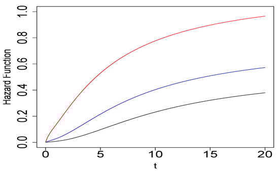
Figure 3. Hazard function of AKS distribution for selected values of $\theta$: $\theta =0.6$ (black color), $\theta =0.8$ (blue color), and $\theta =1.2$ (red color).

Proposition 3. 

Let T∼$AKS\left(\theta \right)$. Then, the hazard function of T is increasing for all $t>0$.

Proof. 

We use the idea from the proof of the theorem in Glaser [19]. Specifically, we define $g\left(t\right)={\displaystyle \frac{1}{h\left(t\right)}}$, where h is the hazard function. The first derivative of g is given by

$$g^{\prime }\left(t\right)=g\left(t\right)\eta \left(t\right)-1,$$

where $\eta \left(t\right)$ is defined as:

$$\begin{array}{c}\hfill \eta \left(t\right)=-{\displaystyle \frac{f^{\prime }\left(t\right)}{f\left(t\right)}}=\theta -{\displaystyle \frac{1}{t}}-{\displaystyle \frac{40t+4t^3}{30+20t^2+t^4}},\end{array}$$

where $f\left(t\right)$ is the pdf given in (7). Using the expressions for $g^{\prime }$ and $\eta$, we can express $g^{\prime }$ as

$$g^{\prime }\left(t\right)={\int }_t^{\infty }[f\left(y\right)/f\left(t\right)]\eta \left(t\right)dy-1.$$

By algebraically manipulating this expression, we obtain

$$g^{\prime }\left(t\right)={\int }_t^{\infty }[f\left(y\right)/f\left(t\right)](\eta \left(t\right)-\eta \left(y\right))dy.$$

(9)

Furthermore, differentiating the function $\eta \left(t\right)$ with respect to t, we have

$$\begin{array}{c}\hfill {\eta }^{\prime }\left(t\right)={\displaystyle \frac{900+900t^4+80t^6+5t^8}{t^2{(30+20t^2+t^4)}^2}}>0,\forall t>0.\end{array}$$

Since ${\eta }^{\prime }\left(t\right)>0$ for all $t>0$, substituting this into (9), shows that $g^{\prime }\left(t\right)<0$ for all $t>0$. Combining this result with the definition of g, the desired result follows.    □

2.4. Order Statistics

Let $Z_1,\dots ,Z_n$ be a random sample of a random variable Z∼$AKS\left(\theta \right)$. Let us denote by $Z_{\left(j\right)}$ the $jth$–order statistics, $j\in \{1,\dots ,n\}$.

Proposition 4. 

The pdf of $Z_{\left(j\right)}$ is

$$\begin{array}{ccc}\hfill f_{Z_{\left(j\right)}}\left(z\right)& =& {\displaystyle \frac{n!{\theta }^{6}zexp(-\theta z)(30+20z^2+z^4)}{(j-1)!(n-j)!{30}^n{({\theta }^2+2)}^{2n}}}{\left\{30{\theta }^4\gamma (2,\theta z)+20{\theta }^2\gamma (4,\theta z)+\gamma (6,\theta z)\right\}}^{j-1}\hfill \\ & \times & {\left\{30{({\theta }^2+2)}^2-30{\theta }^4\gamma (2,\theta z)-20{\theta }^2\gamma (4,\theta z)-\gamma (6,\theta z)\right\}}^{n-j},\hfill \end{array}$$

where $z>0$ and $\theta >0.$ In particular, the pdf of the minimum, $Z_{\left(1\right)}$, is

$$f_{Z_{\left(1\right)}}\left(z\right)={\displaystyle \frac{n{\theta }^{6}zexp(-\theta z)(30+20z^2+z^4)}{{30}^n{({\theta }^2+2)}^{2n}}}{\left\{30{({\theta }^2+2)}^2-30{\theta }^4\gamma (2,\theta z)-20{\theta }^2\gamma (4,\theta z)-\gamma (6,\theta z)\right\}}^{n-1},$$

and the pdf of the maximum, $Z_{\left(n\right)}$, is

$$f_{Z_{\left(n\right)}}\left(z\right)={\displaystyle \frac{n{\theta }^{6}zexp(-\theta z)(30+20z^2+z^4)}{{30}^n{({\theta }^2+2)}^{2n}}}{\left\{30{\theta }^4\gamma (2,\theta z)+20{\theta }^2\gamma (4,\theta z)+\gamma (6,\theta z)\right\}}^{n-1}.$$

Proof. 

Since we are dealing with an absolutely continuous model, the pdf of the $jth$–order statistic is obtained by applying

$$\begin{array}{ccc}\hfill f_{Z_{\left(j\right)}}\left(x\right)& =& \hfill {\displaystyle \frac{n!}{(j-1)!(n-j)!}}f\left(z\right){\left[F\left(z\right)\right]}^{j-1}{[1-F\left(z\right)]}^{n-j},j\in \{1,\dots ,n\}\hfill \end{array}$$

where F and f denote the cdf and pdf of the parent distribution, Z∼$AKS\left(\theta \right)$ in this case.    □

2.5. Moments

In this subsection, we provide the moments, the moment generating function and skewness and kurtosis coefficients.

Proposition 5. 

Let Z∼$AKS\left(\theta \right)$. Then, for $r=1,2,3,\dots ,$ the r-moment of Z is given by

$${\displaystyle \mathbb{E}\left(Z^r\right)=\frac{r!}{{\theta }^r{({\theta }^2+2)}^2}\sum _{k=0}^r\left[{\theta }^2+(k+1)(k+2)\right]\left[{\theta }^2+(r-k+1)(r-k+2)\right].}$$

(10)

Proof. 

Using the representation of Z given in Proposition 1 and the binomial theorem, we have that the r-th moment is

$${\displaystyle \mathbb{E}\left(Z^r\right)=\mathbb{E}\left({(X_1+X_2)}^r\right)=\sum _{k=0}^r\left(\genfrac{}{}{0pt}{}{r}{k}\right)\mathbb{E}\left(X_1^k\right)\mathbb{E}\left(X_2^{r-k}\right).}$$

Then, using the moments of the AK random variable given in (5), the result is obtained.    □

Proposition 6. 

Let Z∼$AKS\left(\theta \right)$. Then, the moment generating function of the random variable Z is given by

$$M_Z\left(t\right)=\mathbb{E}\left(exp\left(tZ\right)\right)={\displaystyle \frac{{\theta }^6}{{({\theta }^2+2)}^2}}{\left[{\displaystyle \frac{{(\theta -t)}^2+2}{{(\theta -t)}^3}}\right]}^2,t<\theta .$$

(11)

Proof. 

Using the representation given in Proposition 1, we get:

$$M_Z\left(t\right)=\mathbb{E}\left(exp\left(tZ\right)\right)=\mathbb{E}\left(exp\left(t(X_1+X_2)\right)\right)=M_{X_1}\left(t\right)M_{X_2}\left(t\right),$$

and using the moment generating function of the AK random variable given in (6), the result follows.    □

Corollary 2. 

Let Z∼$AKS\left(\theta \right)$. Then, the mean and variance Z are given, respectively, by

$$\begin{array}{c}\hfill {\displaystyle \mathbb{E}\left(Z\right)=\frac{2({\theta }^2+6)}{\theta ({\theta }^2+2)}\mathrm{and}Var\left(Z\right)=\frac{2({\theta }^4+16{\theta }^2+12)}{{\theta }^2{({\theta }^2+2)}^2}.}\end{array}$$

The skewness and kurtosis coefficients are, respectively,

$${\displaystyle \sqrt{{\beta }_1}=\frac{\sqrt{2}({\theta }^6+30{\theta }^4+36{\theta }^2+24)}{{({\theta }^4+16{\theta }^2+12)}^{3/2}},}$$

$${\displaystyle {\beta }_2=\frac{6({\theta }^8+40{\theta }^6+172{\theta }^4+240{\theta }^2+96)}{{({\theta }^4+16{\theta }^2+12)}^2}.}$$

Figure 4 depicts plots of skewness and kurtosis coefficients of the AKS distribution.

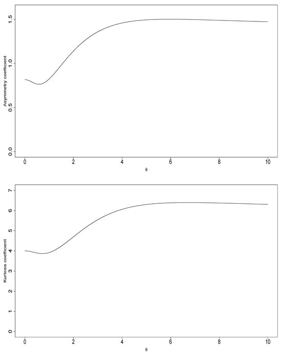
Figure 4. Plots of the skewness and kurtosis coefficients of the $AKS$ model.

3. Inference

In this section, we estimate the $\theta$ parameter of the AKS model using the method of moments (MM) and the maximum likelihood (ML) method. Asymptotic properties of the ML estimator are discussed, and a simulation study is presented. However, before proceeding, we introduce the following technical lemma:

Lemma 1. 

Let $p\left(x\right)=-a{x}^3+2x^2-2ax+12$, where $a>0$. Then, $p\left(x\right)$ has exactly one positive real root.

Proof. 

By direct calculation, the first and second derivatives of p are given by

$$p^{\prime }\left(x\right)=-3a{x}^2+4x-2a\mathrm{and}{p}^{″}\left(x\right)=-6ax+4.$$

We note that if

• $a>\sqrt{{\displaystyle \frac{2}{3}}}$, then the discriminant of $p^{\prime }$ is $\Delta =16-24a^2=8(2-3a^2)<0$. Since its leading coefficient is $-3a<0$, it follows that $p^{\prime }\left(x\right)<0$ for all x. Therefore, since p is decreasing for all x, and given that $p\left(0\right)=12$ and ${\displaystyle \underset{x\to \infty }{lim}p\left(x\right)=-\infty }$, the result follows.
• $0<a<\sqrt{{\displaystyle \frac{2}{3}}}$, the polynomial $p^{\prime }$ has two positive real roots, which are

  $$x_1={\displaystyle \frac{2-\sqrt{4-6a^2}}{3a}}\mathrm{and}{x}_2={\displaystyle \frac{2+\sqrt{4-6a^2}}{3a}}.$$
  Using the second derivative criterion, we find that at $x_1>0$, p reaches a local minimum value, and at $x_2$, p reaches a local maximum value. Moreover, since $p\left(x_1\right)>0$ and ${\displaystyle \underset{x\to \infty }{lim}p\left(x\right)=-\infty }$, the result follows.
• $a=\sqrt{{\displaystyle \frac{2}{3}}}$, the only critical point of p is $x=a$. Since the leading coefficient of $p^{\prime }$ is negative, p is decreasing for all x. Moreover, $x=a$ is an inflection point of p, and since $p\left(a\right)>0$, the result follows.

   □

3.1. Method of Moments

Let $z_1,\dots ,z_n$ be a random sample from Z∼$AKS\left(\theta \right)$. Let $\overline{z}={\displaystyle \frac{{\sum }_{i=1}^n{z}_i}{n}}$ be the first sample moment.

Proposition 7. 

Given $z_1,\dots ,z_n$, a random sample from Z∼$AKS\left(\theta \right)$, the method of moment estimator of θ (${\widehat{\theta }}_M$) provides the following estimator:

$$\begin{array}{ccc}\hfill {\widehat{\theta }}_M& =& {\displaystyle \frac{2}{3\overline{z}}}+{\displaystyle \frac{-4+6{\overline{z}}^2}{3\times 2^{1/3}\overline{z}{(-4-72{\overline{z}}^2+3\sqrt{6}\sqrt{12{\overline{z}}^2+94{\overline{z}}^4+{\overline{z}}^6})}^{1/3}}}\hfill \\ & & -{\displaystyle \frac{2^{1/3}{(-4-72{\overline{z}}^2+3\sqrt{6}\sqrt{12{\overline{z}}^2+94{\overline{z}}^4+{\overline{z}}^6})}^{1/3}}{3\overline{z}}}.\hfill \end{array}$$

Proof. 

The equation for the method of moments is given by

$$\begin{array}{c}\hfill {\displaystyle \mathbb{E}\left[Z\right]=\frac{2({\theta }^2+6)}{\theta ({\theta }^2+2)}=\overline{z},}\end{array}$$

(12)

which can be rewritten as

$$\begin{array}{c}\hfill -\overline{z}{\theta }^3+2{\theta }^2-2\overline{z}\theta +12=0.\end{array}$$

(13)

Solving Equation (13) yields the result, which is the only solution as stated in Lemma 1, considering $a=\overline{z}$ y $x=\theta$.    □

3.2. Maximum Likelihood Estimation

For a random sample, $z_1,\dots ,z_n$, derived from the $AKS(\theta$) distribution, the log-likelihood function can be written as

$$\ell \left(\theta \right)=6nlog\left(\theta \right)+\sum _{i=1}^{n}log\left(z_i\right)-2nlog({\theta }^2+2)-n\overline{z}\theta +\sum _{i=1}^{n}log\left(30+20z_i^2+z_i^4\right)-nlog\left(30\right).$$

The score equation is given by

$$\begin{array}{c}\hfill {\displaystyle \frac{d\ell \left(\theta \right)}{d\theta }}={\displaystyle \frac{6n}{\theta }}-{\displaystyle \frac{4n\theta }{{\theta }^2+2}}-n\overline{z}=0,\end{array}$$

which also yields Equation (13). Thus, the ML estimator for $\theta$ ($\widehat{\theta }$) is also obtained by solving Equation (13). Consequently, the ML estimator of $\theta$ coincides with the moments estimator given in the Proposition 7.

Hence, for large samples, the ML estimator, $\widehat{\theta }$, is asymptotically normal. That is,

$$\sqrt{n}\left(\widehat{\theta }-\theta \right)\stackrel{\mathcal{L}}{⟶}N(0,I_F^{-1}\left(\theta \right)),$$

where the asymptotic variance of the ML estimator $\widehat{\theta }$ is the inverse of Fisher’s information:

$${\displaystyle Var\left(\widehat{\theta }\right)\approx \frac{{\theta }^2{({\theta }^2+2)}^2}{2n({\theta }^4+16{\theta }^2+12)},I_F\left(\theta \right)=\frac{2({\theta }^4+16{\theta }^2+12)}{{\theta }^2{({\theta }^2+2)}^2}.}$$

More precisely, by definition, the Fisher Information is

$$I_F\left(\theta \right)=-\mathbb{E}\left[{\displaystyle \frac{{\partial }^2}{\partial {\theta }^2}}log{f}_Z(z;\theta )\right].$$

For the proposed distribution we have

$$log{f}_Z(z;\theta )=log\left({\displaystyle \frac{{\theta }^{6}z}{30{({\theta }^2+2)}^2}}\right)+log(30+20z^2+z^4)-\theta z.$$

The first and second derivatives of $log{f}_Z(z;\theta )$ are

$${\displaystyle \frac{\partial }{\partial \theta }}log{f}_Z(z;\theta )={\displaystyle \frac{6}{\theta }}-{\displaystyle \frac{4\theta }{{\theta }^2+2}}-z,\mathrm{and}{\displaystyle \frac{{\partial }^2}{\partial {\theta }^2}}log{f}_Z(z;\theta )=-{\displaystyle \frac{6}{{\theta }^2}}+{\displaystyle \frac{4{\theta }^2-8}{{({\theta }^2+2)}^2}}.$$

Consequently, substituting the first and second derivatives in $I_F\left(\theta \right)$, the Fisher information is

$$I_F\left(\theta \right)=-\mathbb{E}\left[{\displaystyle \frac{{\partial }^2}{\partial {\theta }^2}}log{f}_Z(z;\theta )\right]=-\mathbb{E}\left[-{\displaystyle \frac{6}{{\theta }^2}}+{\displaystyle \frac{4{\theta }^2-8}{{({\theta }^2+2)}^2}}\right]={\displaystyle \frac{6}{{\theta }^2}}-{\displaystyle \frac{4{\theta }^2-8}{{({\theta }^2+2)}^2}}={\displaystyle \frac{2{\theta }^4+32{\theta }^2+24}{{\theta }^2{({\theta }^2+2)}^2}}.$$

3.3. Simulation Study

To examine the performance of the ML estimator of the parameter $\theta$ of the AKS distribution, a simulation study is carried out. An algorithm is available to generate random numbers from the AKS distribution. The simulation analysis is performed by generating 1000 samples of sizes $n=20,$ 50, and 100 from the AKS distribution. The algorithm used to generate random numbers from the AKS distribution is shown below. The Algorithm 1 is based on the representation given in Proposition 1, together with the fact that, as seen below Equation (7), the AKS distribution can be represented as a mixture of an exponential and a gamma distribution.

Algorithm 1 for simulating from the Z∼$AKS\left(\theta \right)$ can proceed as follows:

Step 1: Generate $S_i$∼$Exp\left(\theta \right),i=1,2.$ Step 2: Generate $T_i$∼$Gamma(3,\theta ),i=1,2.$ Step 3: Generate $V_i$∼$Bernoulli\left({\displaystyle \frac{\theta }{1+\theta }}\right),i=1,2.$ Step 4: Compute $X_i=V_i{S}_i+(1-V_i)T_i,i=1,2.$ Step 5: Compute $Z=X_1+X_2$

Table 1 shows the empirical bias (B), the average of the standard errors (SE), the empirical root mean squared error (RMSE), and the coverage probability (CP). It is to be noted that the CP converge reasonably well to the nominal value used in their construction (95%), suggesting that the normal distribution is a reasonable asymptotic distribution for the ML estimators in the AKS model. Additionally, Table 1 demonstrates that the value of B becomes quite small as n increases, that the SE and SMSE are almost the same, and that the CP values are close to $95\%$. From this, we can conclude that the estimation method performs very well, even with relatively small sample sizes. All simulations were performed using the R programming language [20].

Table 1. B, SE, RMSE, and CP for the AKS model with $n=20$, 50, and 100.

$\mathit{\theta }$	n	B	SE	RMSE	CP
0.2	20	0.001	0.018	0.018	0.942
	50	0.001	0.012	0.012	0.949
	100	0.0002	0.008	0.008	0.955
0.5	20	0.002	0.046	0.046	0.952
	50	0.001	0.029	0.029	0.952
	100	0.001	0.019	0.019	0.946
0.8	20	0.004	0.073	0.073	0.945
	50	0.002	0.045	0.045	0.957
	100	0.002	0.031	0.031	0.953
1	20	0.007	0.091	0.091	0.955
	50	−0.001	0.056	0.056	0.954
	100	0.004	0.040	0.040	0.941
2	20	0.013	0.204	0.204	0.954
	50	0.007	0.126	0.126	0.943
	100	0.008	0.088	0.088	0.948
3	20	0.051	0.366	0.369	0.943
	50	0.021	0.223	0.224	0.952
	100	0.009	0.155	0.155	0.950
4	20	0.067	0.537	0.540	0.946
	50	0.025	0.323	0.324	0.953
	100	0.028	0.238	0.240	0.949
5	20	0.052	0.688	0.690	0.955
	50	0.049	0.441	0.444	0.954
	100	0.016	0.309	0.309	0.948

4. Applications

In this Section, the AKS distribution is fitted to two engineering science data sets and compared with the AK and L distributions.

4.1. Application 1

In this application, the data set consists of the strength of the glass of the aircraft window reported by Fuller et al. [21]. The data are shown in Table 2.

Table 2. Strength of the glass of aircraft windows reported by Fuller et al. [21].

18.83	20.80	21.657	23.03	23.23	24.05	24.321	25.50	25.52	25.80
26.69	26.77	26.78	27.05	27.67	29.90	31.11	33.20	33.73	33.76
33.89	34.76	35.75	35.91	36.98	37.08	37.09	39.58	44.045	45.29
45.381

Descriptive statistics are given in Table 3, where CS is the sample skewness coefficient, and CK is the sample kurtosis coefficient.

Table 3. Descriptive statistics for the strength of glass data.

n	Median	Mean	Variance	CS	CK
31	29.90	30.81	52.61	0.405	2.287

Table 4 shows the ML estimates of the parameters of the AKS, AK, and L models together with their standard errors in parentheses, and the values of the AIC, BIC, and HQIC criteria are given for each model (Akaike information criterion (AIC) introduced by Akaike [22], Bayesian information criterion (BIC) proposed by Schwarz [23] and the Hannan-Quinn Information Criterion (HQIC) introduced by Hannan and Quinn [24]).

Table 4. ML Estimates of the AKS, AK, and L models for glass strength data.

Model	ML Estimate	AIC	BIC	HQIC
AKS($\theta$)	$\widehat{\theta }$ = 0.192(0.014)	225.868	227.302	226.336
AK($\theta$)	$\widehat{\theta }$ = 0.097(0.010)	242.682	244.116	243.149
L($\theta$)	$\widehat{\theta }$ = 0.063(0.008)	255.988	257.422	256.456

Note that the lowest values of AIC, BIC, and HQIC correspond to the AKS model, indicating that this model provides a better fit compared to the AK and L models.

For the fitted AKS distribution, we calculated the quantile residuals (QR). If the model is appropriate for the data, the QRs should be a sample from the standard normal model (see Dunn and Smyth [25]). To verify that the QRs are normally distributed, we apply several traditional tests, such as the Anderson–Darling (AD), Cramér–von Mises (CVM), Shapiro–Wilk (SW), and Kolmogorov–Smirnov (KS) tests.

In Figure 5, the QRs for the AKS distribution are shown together with the p-values (in parentheses) of the AD, CVM, SW, and KS normality tests. It is seen that the AKS distribution verifies the assumption that the QRs come from the standard normal distribution, validating the fit of the AKS distribution to the strength of glass data.

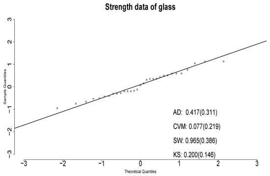
Figure 5. Q-Q plots of the QRs for AKS distribution.

4.2. Application 2

In this application, we model a data set collected by the Department of Mines of the University of Atacama, Chile. The data consisting of yttrium measurements in 86 samples of mineral, which are presented in Table 5.

Table 5. Yttrium data collected by the Mines Department, University of Atacama, Chile.

27	20	17	12	33	19	27	27	25	26
17	13	15	22	24	20	9	20	13	26
8	27	29	7	33	28	15	36	31	24
22	12	26	35	15	45	10	27	24	42
27	23	16	18	28	17	30	18	19	10
30	30	12	20	17	26	23	35	33	18
12	22	30	15	19	32	19	19	50	24
17	34	29	34	32	12	44	39	34	16
31	22	20	17	18	25

Summary statistics are reported in Table 6. ML estimates of the parameter of the AKS, AK, and L models together with their SE and the values of the AIC, BIC, and HQIC are given in Table 7.

Table 6. Descriptive statistics for yttrium data.

n	Median	Mean	Variance	CS	CK
86	23.00	23.53	79.264	0.489	3.033

Table 7. ML Estimates of AKS, AK, and L models for yttrium data.

Model	ML Estimate	AIC	BIC	HQIC
AKS($\theta$)	$\widehat{\theta }=0.250\left(0.011\right)$	617.956	620.411	618.944
AK($\theta$)	$\widehat{\theta }=0.127\left(0.008\right)$	640.645	643.100	641.633
L($\theta$)	$\widehat{\theta }=0.082\left(0.006\right)$	669.327	671.781	670.314

We observe that the smallest values of the AIC, BIC, and HQIC criteria correspond to the AKS model, indicating that the AKS model provides a better fit to the data compared to the AK and L models.

The residual quantiles of the AKS distribution are shown in Figure 6. Also, the p-values for the AD, CVM, SW, and KS normality tests are given to verify if the QRs come from a standard normal distribution. These indicate that the AKS distribution provides a good fit for the yttrium data.

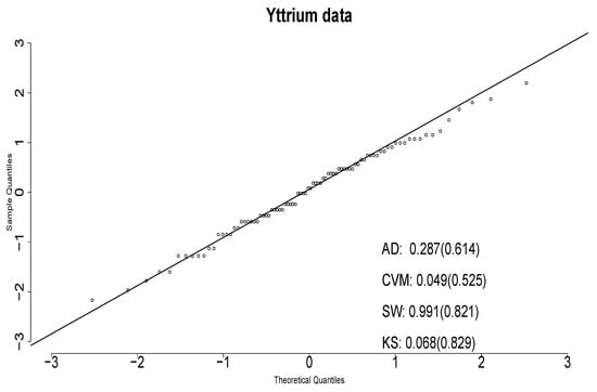
Figure 6. Q–Q plots of the QRs for AKS distribution.

5. Conclusions

In this article, we have studied the convolution of two independent AK random variables with a parameter in common. We have given some of the properties of the new AKS distribution and developed parameter estimates by the methods of moments and maximum likelihood. A simulation study was carried out to investigate the performance of the ML estimator. Also, the ability of the AKS distribution was demonstrated in two applications made on real data sets. It consistently produced better fits than the AK and L distributions.

Some additional features of the AKS are:

• The AKS distribution has a simple representation.
• The cumulative distribution and risk functions are explicit and represented by known functions.
• The moments and ML estimators coincide and have closed-form solutions.
• The ML estimator performs very well, even when the samples are small.
• The AIC, BIC, and HQIC model selection criteria indicate that in both applications, the AKS distribution provides a better fit to the data compared to the AK and L models. Additionally, the Anderson–Darling, Cramér–von Mises, Shapiro–Wilk, and Kolmogorov–Smirnov tests confirm that the quantile residuals follow a standard normal distribution.
• A future study could, for example, explore the sum of two AK distributions with different parameters, thereby obtaining a two-parameter distribution.

References

- Lindley, D.V. Fiducial distributions and Bayes’ theorem. J. R. Stat. Soc. Ser. B 1958, 20, 102–107. [Google Scholar] [CrossRef]
- Hussain, E. The Non-Linear Functions of Order Statistics and Their Properties in Selected Probability Models. Ph.D Thesis, Department of Statistics, University of Karachi, Karachi, Pakistan, 2006. [Google Scholar]
- Ghitany, M.E.; Atieh, B.; Nadarajah, S. Lindley distribution and its applications. Math. Comput. Simul. 2008, 78, 493–506. [Google Scholar] [CrossRef]
- Zakerzadeh, H.; Dolati, A. Generalized Lindley distribution. J. Math. Ext. 2009, 3, 13–25. [Google Scholar]
- Gómez-Déniz, E.; Calderin-Ojeda, E. The discrete Lindley distribution: Properties and application. J. Stat. Comput. Simul. 2011, 81, 1405–1416. [Google Scholar] [CrossRef]
- Krishna, H.; Kumar, K. Reliability estimation in Lindley distribution with progressively type II right censored sample. Math. Comput. Simulat. 2011, 82, 281–294. [Google Scholar] [CrossRef]
- Bakouch, H.S.; Al-Zaharani, B.; Al-Shomrani, A.; Marchi, V.; Louzada, F. An extended Lindley distribution. J. Korean Stat. Soc. 2012, 41, 75–85. [Google Scholar] [CrossRef]
- Shanker, R.; Sharma, S.; Shanker, R. A two-parameter Lindley distribution for modeling waiting and survival times data. Appl. Math. 2013, 4, 363–368. [Google Scholar] [CrossRef]
- Ghitany, M.; Al-Mutairi, D.; Balakrishnan, N.; Al-Enezi, I. Power Lindley distribution and associated inference. Comput. Stat. Data Anal. 2013, 64, 20–33. [Google Scholar] [CrossRef]
- Al-Mutairi, D.K.; Ghitany, M.E.; Kundu, D. Inferences on stress-strength reliability from Lindley distributions. Commun. Stat.-Theory Methods 2013, 42, 1443–1463. [Google Scholar] [CrossRef]
- Oluyede, B.O.; Yang, T. A new class of generalized Lindley distribution with applications. J. Stat. Comput. Simul. 2014, 85, 2072–2100. [Google Scholar] [CrossRef]
- Shanker, R.; Hagos, F.; Sujatha, S. On modeling of Lifetimes data using exponential and Lindley distributions. Biom. Biostat. Int. J. 2015, 2, 1–9. [Google Scholar] [CrossRef]
- Abouammoh, A.M.; Alshangiti, A.M.; Ragab, I.E. A new generalized Lindley distribution. J. Stat. Comput. Simul. 2015, 85, 3662–3678. [Google Scholar] [CrossRef]
- Shanker, R. Akash Distribution and Its Applications. Int. J. Probab. Stat. 2015, 4, 65–75. [Google Scholar]
- Shanker, R.; Shukla, K.K. On Two-Parameter Akash Distribution. Biom. Biostat. Int. J. 2017, 6, 00178. [Google Scholar] [CrossRef][Green Version]
- Shanker, R.; Shukla, K.K. Power Akash Distribution and Its Application. J. Appl. Quant. Methods 2017, 12, 1–10. [Google Scholar]
- Gómez, Y.M.; Firinguetti-Limone, L.; Gallardo, D.I.; Gómez, H.W. An Extension of the Akash Distribution: Properties, Inference and Application. Mathematics 2014, 12, 31. [Google Scholar] [CrossRef]
- Yaghoubi, A. Sum of Independent Random Variable for Shanker, Akash, Ishita, Pranav, Rani and Ram Awadh Distributions. arXiv 2022, arXiv:2208.08006. [Google Scholar]
- Glaser, R.E. Bathtub and Related Failure Rate Characterizations. J. Am. Stat. Assoc. 1980, 75, 667–672. [Google Scholar] [CrossRef]
- R Core Team. R: A Language and Environment for Statistical Computing; R Foundation for Statistical Computing: Vienna, Austria, 2023; Available online: https://www.R-project.org/ (accessed on 8 June 2024).
- Fuller, E.R., Jr.; Frieman, S.; Quinn, J.; Quinn, G.; Carter, W. Fracture mechanics approach to the design of glass aircraft windows: A case study, SPIE Procceding. In Window and Dome Technologies and Materials IV; SPIE: Bellingham, WA, USA, 1994; Volume 2286, pp. 419–430. [Google Scholar] [CrossRef]
- Akaike, H. A new look at the statistical model identification. IEEE Trans. Automat. Contr. 1974, 19, 716–723. [Google Scholar] [CrossRef]
- Schwarz, G. Estimating the dimension of a model. Ann. Stat. 1978, 6, 461–464. [Google Scholar] [CrossRef]
- Hannan, E.J.; Quinn, B.G. The Determination of the order of an autoregression. J. R. Stat. Soc. Series B 1979, 41, 190–195. [Google Scholar] [CrossRef]
- Dunn, P.K.; Smyth, G.K. Randomized Quantile Residuals. J. Comput. Graph. Stat. 1996, 5, 236–244. [Google Scholar] [CrossRef]
Disclaimer/Publisher’s Note: The statements, opinions and data contained in all publications are solely those of the individual author(s) and contributor(s) and not of MDPI and/or the editor(s). MDPI and/or the editor(s) disclaim responsibility for any injury to people or property resulting from any ideas, methods, instructions or products referred to in the content. |
© 2025 by the authors. Licensee MDPI, Basel, Switzerland. This article is an open access article distributed under the terms and conditions of the Creative Commons Attribution (CC BY) license (https://creativecommons.org/licenses/by/4.0/).