Article

On the Bayesian Two-Sample Problem for Ranking Data

Department of Mathematics and Statistics, University of Ottawa, Ottawa, ON K1N 6N5, Canada
Axioms 2025, 14(4), 292; https://doi.org/10.3390/axioms14040292
Submission received: 20 February 2025 / Revised: 24 March 2025 / Accepted: 29 March 2025 / Published: 14 April 2025

Abstract

We consider the two-sample problem involving a new class of angle-based models for ranking data. These models are functions of the cosine of the angle between a ranking and a consensus vector. A Bayesian approach is employed to determine the corresponding predictive densities. Two competing hypotheses are considered, and we compute the Bayes factor to quantify the evidence provided by the observed data under each hypothesis. We apply the results to a real data set.

1. Introduction

Ranking data have been frequently collected and analyzed in a variety of different contexts, including problems of trend, market research, politics and judging situations. A comprehensive discussion of various probability ranking models may be found in Alvo and Yu [1], whereas Fagin et al. [2] considered models for the distribution of rankings for the top-k items. In the present context, scores are assigned to items to reflect their relative preference. The probability of observing a ranking is modeled to be a function of the cosine of the angle between the vector of scores and a consensus score vector denoted by θ . A Bayesian approach is then taken wherein a joint von Mises–Fisher prior distribution is placed on the parameters. The estimation is subsequently conducted by making use of the variational inference method. The model is successfully applied to the Sushi data set.
In the present article, our attention is focused on the two-sample problem for ranking data, and the interest is in quantifying the evidence for two competing hypotheses. This is achieved by computing Bayes factors. In Section 2, we first describe the one-sample angle-based model, as well as the Bayesian MCMC approach. In Section 3, we describe the Bayesian two-sample problem and propose the use of Bayes factors to quantify the evidence provided by data in favor of one hypothesis compared to another. In Section 4, we describe an application of the two-sample model to the well-known Sushi data set. We conclude with a discussion in Section 5.

2. One-Sample Angle-Based Model

In this section, we recall the one-sample problem. A ranking for t items labeled 1 , , t , R = ( R ( 1 ) , , R ( t ) ) T may be viewed as a permutation of the integers 1 , , t , which may be conveniently expressed in standardized form as
y = R t + 1 2 t ( t 2 1 ) 12 ,
where y is the t × 1 vector with y = 1 . The probability distribution of the ranking y may be modeled as follows:
p ( y | κ , θ ) = C ( κ , θ ) exp κ θ T y
where the parameter θ may be interpreted as a t × 1 “consensus” vector with θ = 1 , parameter κ 0 , and C ( κ , θ ) is the normalizing constant. Since both θ and y are standardized geometrically, the cosine of the angle between the consensus score vector θ and the observation y is given by θ T y . The parameter κ can be viewed as a concentration parameter. A small value of κ implies that the distribution of rankings is uniform, whereas a large value of κ points to a distribution that is more concentrated around the consensus score vector. The normalizing constant is computed by summing exp κ θ T y over all t ! possible permutations of the integers 1 , , t . For large values of t, this becomes prohibitive.
The model in (1) closely resembles the continuous von Mises–Fisher distribution, abbreviated as v M F ( x | m , κ ) , which is defined on a p 1 -dimensional unit sphere with mean direction m and concentration parameter κ :
p ( x | κ , m ) = V p ( κ ) exp ( κ m T x ) ,
where
V p ( κ ) = κ p 2 1 2 π p 2 I p 2 1 ( κ ) ,
and I p 2 1 ( κ ) is the modified Bessel function of the first kind with order p 2 1 . Consequently, as shown in Xu et al. [3], we may approximate the normalizing constant in the discrete model by
C ( κ , θ ) C t ( κ ) = κ t 3 2 2 t 3 2 t ! I t 3 2 ( κ ) Γ ( t 1 2 ) ,
where Γ ( · ) is the gamma function.

2.1. Maximum Likelihood Estimation (MLE)

The estimation of the parameters κ , θ in (1) proceeds by making use of the method of maximum likelihood. Let Y = y 1 , , y N be a random sample of N standardized rankings drawn from p ( y | κ , θ ) . Then, the log-likelihood of κ , θ is given by
L ( y | κ , θ ) = N ln C t ( κ ) + i = 1 N κ θ T y i .
The maximum likelihood estimator of θ subject to θ = 1 and κ 0 is given by
θ ^ M L E = i = 1 N y i i = 1 N y i ,
whereas κ ^ is calculated from the relation
A t ( κ ) C t ( κ ) C t ( κ ) = I t 1 2 κ I t 3 2 κ = i = 1 N y i N r
Whereas Banerjee et al. [4] proposed
κ ^ M L E = r ( t 1 r 2 ) 1 r 2
a more precise approximation can be obtained recursively as
κ i + 1 = κ i A t ( κ i ) r 1 A t ( κ i ) 2 t 2 κ i A t ( κ i ) , i = 0 , 1 , 2 , .

2.2. Bayesian Method with Conjugate Prior

Define a conjugate prior for ( κ , θ ) as follows:
p ( κ , θ ) = p ( θ | κ ) p ( κ ) = v M F ( θ | m 0 , β 0 κ ) G ( κ | a 0 , b 0 ) ,
where G ( κ | a 0 , b 0 ) is the gamma density function with shape parameter a 0 and rate parameter b 0 and a mean equal to a 0 b 0 . Given Y = y , the posterior density of ( κ , θ ) can be expressed by
p ( κ , θ | y ) exp β κ m T θ V t ( β κ ) C t ( κ ) N + ν 0 V t ( β κ ) ,
where m = β 0 m 0 + i = 1 N y i β 1 ,   β = β 0 m 0 + i = 1 N y i . The posterior density can be factorized as
p ( κ , θ | y ) = p ( θ | κ , y ) p ( κ | y ) ,
where p ( θ | κ , y ) v M F ( θ | m , β κ ) and
p ( κ | y ) C t ( κ ) N + ν 0 V t ( β κ ) = κ t 3 2 ( υ 0 + N ) I t 2 2 ( β κ ) I t 3 2 ( κ ) ν 0 + N β κ t 2 2
It is not possible to compute the normalizing constant for p ( κ | Y ) ) in closed form. Nunez-Antonio and Gutiérrez-Pena [5] exploited a sampling importance resampling (SIR) procedure with a proposal density chosen to be the gamma density with variance equal to some pre-specified number such as 50 or 100. However, this choice for the variance is crucially related to the performance of SIR. An improper choice of variance may lead to slow or unsuccessful convergence. Moreover, the MCMC method led to intensive computational complexity. Furthermore, β κ can be very large if N is large, which complicates the computation of the term V t ( β κ ) . Thus, it would not be possible to calculate the weights in the SIR method when N is large. As a result, the posterior distribution was approximated using the method of variational inference (abbreviated as VI henceforth).
As shown in (Xu et al. [3]), p ( κ | Y ) ) can be approximated by G a m m a ( κ | a , b ) with shape a and rate b, where the posterior mode κ ¯ is
κ ¯ = a 1 b if a > 1 , a b otherwise
and
a = a 0 + N t 3 2 + β κ ¯ β κ ln I t 2 2 ( β κ ¯ ) ,
b = b 0 + N κ I t 3 2 ( κ ¯ ) + β 0 β 0 κ ln I t 2 2 ( β 0 κ ¯ ) .
Here, we approximated the posterior distribution by making use of variational inference, which has been used in many applications. In the variational inference approach, we first propose a candidate family of densities and then select the member of that family that comes closest to the target posterior density in the Kullback–Leibler sense. Specifically, let q Z represent the candidate family and suppose that p Z | Y represents the target posterior density. Then, the Kullback–Leibler divergence is given by
K L q | p = E q ln q Z p Z | Y .
For further background on Bayesian methods, see Gelman et al. [6].

3. Two-Sample Problem

In the two-sample problem, there are two independent random samples Y i = y i 1 , , y i N i for i = 1 , 2 of standardized rankings each drawn, respectively, from p ( y i | κ , θ i ) . Conditional on κ , we assume that there are independent von Mises conjugate priors, respectively, for ( θ 1 , θ 2 ) as
p ( θ i | κ ) C t ( κ ) ν 0 exp κ m 0 T θ i ,
where m 0 = 1 , ν 0 , 0 . To motivate interest in the two-sample problem, we shall investigate the difference in food preference patterns with respect to Sushi between Eastern and Western Japan. Individual models are first fitted to each sample. Then, we are interested in comparing the parameters θ 1 , θ 2 .
The Bayes factor is a statistical measure used in Bayesian analysis to quantify the evidence in favor of one hypothesis compared to another. It compares the likelihood of the observed data under two competing hypotheses, typically the null hypothesis H 0 vs. the alternative hypothesis H 1 . The Bayes factor is defined as the ratio of the likelihoods under the alternative and the null hypothesis, respectively:
B F = P ( D a t a H 1 ) P ( D a t a H 0 )
Bayes factors are widely used for model selection, hypothesis testing, and decision-making within the Bayesian framework; see Kass and Raftery [7]. They provide a ratio of how much more (or less) likely the data are under one hypothesis compared to the other. Unlike p-values, they provide a continuous measure of evidence and allow for a direct comparison between hypotheses that incorporate prior beliefs. They penalize overfitting by integrating over parameters, thereby discouraging overly complex models.
Bayes factors have diverse applications across various domains in statistics, science, and decision-making—for example, in testing the effectiveness of a new drug compared to a placebo; in model selection; to evaluate multiple competing models in psychology and cognitive science; in forensic science, genetics, and bioinformatics; in econometrics; and, finally, in artificial intelligence and machine learning. By quantifying evidence in a probabilistic manner, Bayes factors offer an intuitive and rigorous alternative to approaches that make use of p-values. A somewhat practical interpretation scale is as follows.
CriterionInterpretation
1 ≤ BF < 3Weak evidence for H 1
3 ≤ BF < 10Moderate evidence for H 1
BF ≥ 10Strong evidence for H 1
BF < 1/3Moderate evidence for H 0
BF < 1/10Strong evidence for H 0
The Bayes factor was computed in order to compare the following two models. Under model 1, denoted M 1 ,   θ 1 = θ 2 , whereas, under model 2, denoted M 2 , equality is not assumed. We are concerned with the conditional Bayes factor given κ between the two models. The Bayes factor enables us to compute the posterior odds of M 2 to M 1 . It is defined as the ratio of the predictive densities of M 2 to M 1 , namely
B 21 κ = p ( y 1 | κ , θ 1 ) p ( y 2 | κ , θ 2 ) p ( θ 1 , θ 2 | κ | y 1 y 2 ) d θ 1 d θ 2 p ( y 1 | κ , θ ) p ( y 2 | κ , θ ) p ( θ | κ , y 1 y 2 ) d θ
Consider
p ( y 1 | κ , θ 1 ) p ( θ 1 | κ | y 1 ) d θ 1 = C t N 1 κ V t κ e x p κ θ 1 T i y 1 i + β 0 m 0 d θ 1 = C t N 1 κ V t κ V t 1 κ β 1
where
β 1 = i y 1 i + β 0 m 0
Similarly,
p ( y 1 | κ , θ 2 ) p ( θ 2 | κ | Y 2 ) d θ 2 = C t N 2 κ V t κ V t 1 κ β 2
where
β 2 = i y 2 i + β 0 m 0
Consequently, the numerator under model M 2 is given by
C t N 1 κ V t κ V t 1 κ β 1 C t N 2 κ V t κ V t 1 κ β 2
As for the denominator in B 21 ,
p ( y 1 | κ , θ ) p ( y 2 | κ , θ ) p ( θ | κ | ) d θ = C t N 1 + N 2 κ V t κ e x p κ θ T i y 1 i + i y 2 i + β 0 m 0 d θ = C t N 1 + N 2 κ V t κ V t 1 κ β
where
β = i y 1 i + i y 2 i + β 0 m 0
It follows that the conditional Bayes factor given κ is the ratio
B 21 κ = C t N 1 κ V t κ V t 1 κ β 1 C t N 2 κ V t κ V t 1 κ β 2 C t N 1 + N 2 κ V t κ V t 1 κ β = V t κ β V t κ V t κ β 1 V t κ β 2 = β κ p 2 1 2 π p 2 I p 2 1 ( β κ ) κ p 2 1 2 π p 2 I p 2 1 ( κ ) β 1 κ p 2 1 2 π p 2 I p 2 1 ( β 1 κ ) β 2 κ p 2 1 2 π p 2 I p 2 1 ( β 2 κ ) = β β 1 β 2 p 2 1 I p 2 1 ( β 1 κ ) I p 2 1 ( β 2 κ ) I p 2 1 ( β κ ) I p 2 1 ( κ )
where p = t 1 .
There is an approximation to the Bessel functions for a large x:
I p 2 1 ( x ) e x 2 π x
In this case, for a large κ , the conditional Bayes factor is approximately
B 21 κ = β β 1 β 2 p 2 1 I p 2 1 ( β 1 κ ) I p 2 1 ( β 2 κ ) I p 2 1 ( β κ ) I p 2 1 ( κ ) β β 1 β 2 p 1 2 e β 1 + β 2 β 1 κ

4. Application

Using the mixture ranking model, we were interested in uncovering differences in the food preference patterns between Eastern and Western Japan. We made use of the two Sushi data sets of Kamishima and Akaho [8]. Historically, Western Japan has been mainly affected by the culture of the Mikado emperor and nobles, while Eastern Japan was the home of the Shogun and Samurai warriors. Therefore, the preference patterns in food are different between these two regions [8].
We made use of the complete rankings of t = 10 different types of sushi given by 5000 respondents according to their preferences as two samples distinguished by region. There were N 1 = 3285 respondents from Eastern Japan and N 2 = 1715 from Western Japan. We applied the approach described earlier to both the Eastern and Western Japan data. The sample sizes are quite large compared to t, and, consequently, the estimated models for all three methods are quite similar. In Figure 1, we present the posterior means of θ between Eastern Japan (blue bar) and Western Japan (red bar). A more negative value of θ i implies that sushi i is more preferred. Eastern and Western Japan differ mostly in their preferences for salmon roe, squid, sea eel, shrimp, and tuna. Respondents from Eastern Japan prefer salmon roe and tuna more than those from Western Japan, who exhibit a greater preference for squid, shrimp, and sea eel. From Table 1, we see the larger posterior mean of κ , which shows that the Eastern Japanese are slightly more cohesive in their preferences than the Western Japanese in their preferences.
The boxplots of the top smallest posterior means are displayed in Figure 2. Eastern and Western Japan appear to differ mostly in their preferences for sea eel, salmon roe, tuna, sea urchin, and sea bream. The Eastern Japanese exhibit a greater preference for salmon roe, tuna, and sea urchin sushi, whereas the Western Japanese like sea eel and sea bream. Generally, tuna and sea urchin are oilier foods, whereas salmon roe and tuna are more seasonal. So, from the analysis of both data sets, we can conclude that the Eastern Japanese prefer more oily and seasonal food compared to the Western Japanese [8]. The boxplots in Figure 2 also provide a measure of the uncertainty in the values of the θ i s .
We computed the Bayes factor (3) using β 0 = 0 , β = 2209.22 , κ = 4.7 . We have that
B 21 κ 3.6 × 10 11
This leads to favoring the M 1 model, namely that θ 1 = θ 2 . The calculation of the Bayes factor comparing the two models supports the conclusion reached in the original paper.

5. Conclusions and Discussion

We considered the two-sample ranking data problem using angle-based ranking models. Each model is itself a function of a consensus score vector θ , which exhibits detailed information on item preferences, unlike a distance-based model, which only provides an equally spaced modal ranking. We proceeded with a Bayesian approach and placed a conjugate prior on the parameters. We then postulated two different hypotheses and proceeded with the calculation of Bayes factors to compare them. Unlike p-values, Bayes factors provide a continuous measure of evidence between hypotheses that incorporate prior beliefs. We made use of Bayesian variational inference to approximate both the posterior density and the predictive density. We applied our results to the popular sushi data and compared the food preferences of Western and Eastern Japanese consumers.
In further research, it would be of interest to incorporate additional arguments or covariates into the model. These could include judge-specific covariates such as age, gender, and income, whereas item-specific covariates could be prices, weights, and brands. The combination of judge–item covariates could include personal experience on using each phone or brand. The addition of these covariates in the model may greatly enhance the predictive power of the model. Finally, research could explore score functions based on the Kendall distance to enhance ranking comparisons.

Funding

This research was supported by the Natural Sciences and Engineering Research Council of Canada OGP0009068.

Data Availability Statement

Data is contained within the article.

Acknowledgments

The author would like to thank the Natural Sciences and Engineering Research Council of Canada OGP0009068.

Conflicts of Interest

The author declares no conflicts of interest.

References

  1. Alvo, M.; Yu, P. Statistical Methods for Ranking Data; Springer: New Yrok, NY, USA, 2014. [Google Scholar]
  2. Fagin, R.; Kumar, R.; Sivakumar, D. Comparing top k lists. SIAM J. Discret. 2003, 17, 134–160. [Google Scholar] [CrossRef]
  3. Xu, H.; Alvo, M.; Yu, P. Angle-based models for ranking data. Comput. Stat. Data Anal. 2018, 121, 113–136. [Google Scholar]
  4. Banerjee, A.; Dhillon, I.; Ghosh, J.; Sra, S. Clustering on the unit hypersphere using von Mises-Fisher distributions. J. Mach. Learn. Res. 2005, 6, 1345–1382. [Google Scholar]
  5. Nunez-Antonio, G.; Gutiérrez-Pena, E. A bayesian analysis of directional data using the von misesfisher distribution. Commun.-Stat.-Simul. Comput. 2005, 34, 989–999. [Google Scholar] [CrossRef]
  6. Gelman, A.; Carlin, J.B.; Stern, H.S.; Rubin, D.B. Bayesian Data Analysis; CRC Press: Boca Raton, FL, USA, 2013. [Google Scholar]
  7. Kass, R.E.; Raftery, A.E. Bayes factors. J. Am. Stat. Assoc. 1995, 90, 773–795. [Google Scholar]
  8. Kamishima, T.; Akaho, S. Efficient clustering for orders. In Proceedings of the 2nd International Workshop on Mining Complex Data, Hong Kong, China, 18–22 December 2006; pp. 274–278. [Google Scholar]
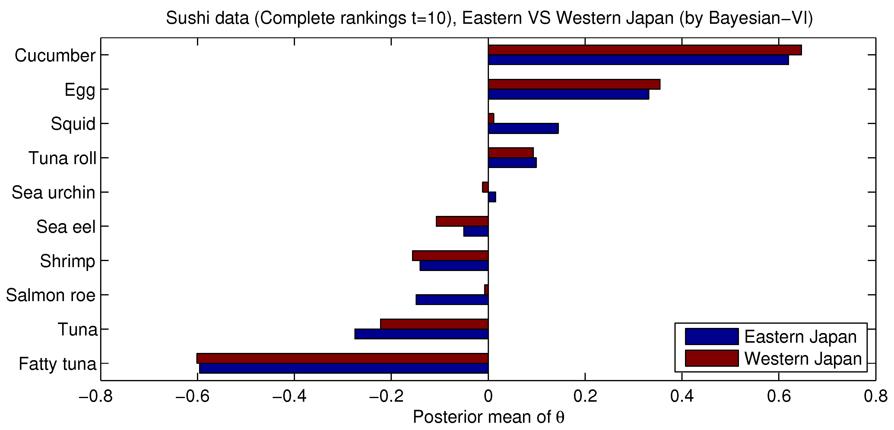
Figure 1. Posterior means of θ for the sushi complete ranking data ( t = 10 ) in Eastern Japan (blue bar) and Western Japan (red bar) obtained by Bayesian-VI.
Axioms 14 00292 g001
Figure 2. Boxplots of the top 10 smallest posterior means of θ for the sushi incomplete rankings ( t = 100 ). Eastern Japan is shown in blue, where circles indicate outliers. Western Japan is shown in red, where red pluses indicate outliers.
Axioms 14 00292 g002
Table 1. Posterior parameters for the sushi complete ranking data ( t = 10 ) in Eastern Japan and Western Japan obtained by Bayesian-VI.
Posterior ParameterEastern JapanWestern Japan
β 1458.85741.61
a18,509.849462.70
b3801.572087.37
Posterior Mean of κ 4.874.53
Disclaimer/Publisher’s Note: The statements, opinions and data contained in all publications are solely those of the individual author(s) and contributor(s) and not of MDPI and/or the editor(s). MDPI and/or the editor(s) disclaim responsibility for any injury to people or property resulting from any ideas, methods, instructions or products referred to in the content.